Sliding Mode Control of Manipulator Based on Improved Reaching Law and Sliding Surface

Abstract

Aiming at the problem of convergence speed and chattering in sliding mode variable structure control of manipulator, an improved exponential reaching law and nonlinear sliding surface are proposed, and the Lyapunov function is used to analyze its stability. According to the dynamic model of the 6-DOF UR5 manipulator and the proposed reaching law and sliding surface, the corresponding control scheme is designed. The control performance of the proposed control scheme is verified by tracking the end trajectory of the manipulator on the MATLAB and CoppeliaSim robot simulation platform. The experimental results show that the proposed control scheme can not only significantly improve the convergence speed and make the system converge quickly, but also can effectively reduce the chattering of the system. Even in the presence of disturbance signals, fast and stable tracking can be achieved while ensuring the robustness of the system, and the chattering of the robotic arm system can be weakened to a certain extent. Compared with the classical control method based on the computational torque method and the traditional sliding mode control scheme based on the exponential reaching law, the proposed scheme has certain advantages in terms of tracking accuracy, convergence speed, and reducing system chattering, and effectively improves the overall control performance of the system.

1. Introduction

The manipulator system is a complex multi-input multi-output, strongly coupled uncertain nonlinear system. Its uncertainty mainly includes two aspects: structural uncertainty and non-structural uncertainty. The former generally includes unmodeled dynamics, dynamic and static friction, system parameter perturbation, etc. The latter is generally caused by external operating environment interference, measurement error, sampling delay, actuator saturation, and other factors. In the industrial field, there are many studies on the traditional control methods of the manipulator, including PID control [1,2,3,4], discrete control [5], adaptive backstepping control [6], feedback linearization [7], robust control [8,9,10,11], neural network control and fuzzy control [12], iterative learning control [13], and variable structure control [14]. PID control is mainly suitable for linear systems, it is only suitable for relatively simple applications, and cannot control objects with complex, large inertia, and large lag [15]. Discrete control is controlled step by step by sampling, and it can effectively suppress noise and has good anti-interference ability [16]. Adaptive backstepping control is introduced into virtual control, and the system is decomposed into simple and low order systems for effective control [17]. Feedback linearization is to linearize the state equation and the output equation; it is a more common linearization method, which can overcome the problem that the error of ordinary linearization increases with the increase of the working area. However, feedback linearization cannot be applied to all nonlinear systems and the states must be all measurable. When there is parameter perturbation, the robustness of the system cannot be guaranteed. Robust control is insensitive to external disturbances and parameter perturbations and is suitable for systems where the range of uncertain factors varies greatly. Because the system using robust control generally does not work in the optimal state, it cannot guarantee that the system has high steady-state accuracy [18]. Neural network and fuzzy control can solve complex nonlinear problems by simulating human intelligent behavior. By designing a reasonable network structure, the optimal parameters of the control system can be well approximated to ensure the control accuracy of the system [19]. Iterative learning control is suitable for solving the problems of control objects with repetitive motion, especially for solving complex nonlinear, strong coupling, and difficult modeling problems. Like robust control, it can deal with uncertainties in the system and can make the system have high steady-state accuracy and achieves full tracking [20]. By combining these control methods, many different control methods will be derived. It also brings many possibilities to effectively and accurately solve the trajectory tracking control problem of the manipulator.

Sliding mode variable structure control has been widely and deeply studied by scholars in the field of robot control because of its strong robustness, insensitivity to parameter changes and disturbances, simple physical structure, no need for accurate physical models, fast response, and other excellent control characteristics. Slotine et al. [21] used the sliding mode control method to conduct the simulation experiment for the two-link manipulator with parameter perturbation and external disturbance. The results show that the proposed method is effective in tracking the desired trajectory. A terminal sliding mode control method is proposed in [22], which realizes the finite-time convergence and stability of the system, but singular problems occur when the control law approaches the ideal sliding surface. Feng et al. [23] proposed a non-singular terminal sliding mode control method, which effectively solved the singularity problem in terminal sliding mode control by introducing appropriate fractional exponents into the control law. However, the chattering problem of sliding mode control is inevitable in these control methods, which leads to the decline of control performance and even makes the system lose stability.

In order to solve the problems of convergence speed and chattering in sliding mode controller, scholars in the control field have proposed various reaching laws. Gao et al. [24] introduced the concept of reaching law for the first time for nonlinear systems and verified the validity of the sliding mode control algorithm based on exponential reaching law. It guarantees the dynamic quality of the reaching process and reduces the chattering of the system. Hong et al. [25] proposed a power reaching law to weaken the chattering of the system. Although the chattering of the system is weakened, the robustness of the system near the sliding mode surface is reduced due to the existence of fractional powers. It increases the time for the system state to reach the sliding mode surface and reduces the convergence speed of the system. In [26], a new reaching law is designed, which includes the exponential term function of the sliding surface. The exponential term can smoothly adapt to the changes of the sliding surface and weaken the system chattering to a certain extent. The reaching law based on discrete-time sliding mode control proposed in [27] reduces the chattering of the system. However, it increases the time for the system state to slide along the sliding hyperplane to the equilibrium point and reduces the speed of the system reaching the sliding surface. Lam et al. [28] designed a sliding mode controller based on the power reaching law for the trajectory tracking control of the dual-arm manipulator, which verifies the effectiveness of the control algorithm. It reduces the tracking error and improves the tracking accuracy of the system, but the system still has chattering that cannot be ignored. Devika et al. [29] proposed an improved exponential reaching law for the slow approaching speed of the traditional reaching law, which improves the approaching speed of the control system, and the system state can quickly reach the sliding mode surface. It improves the speed of system convergence, but the system still has inevitable chattering and the tracking accuracy is not very high.

Based on the discussion of the above problems, this study proposes a new control scheme for the manipulator system. It not only ensures the robustness and control accuracy of the system but also improves the convergence speed of the manipulator system and greatly reduces the chattering of the system. Compared with previous studies, the main contributions of this study are presented below: (1) An improved exponential reaching law is proposed to weaken the system chattering by adjusting the appropriate boundary layer thickness and boundary layer thickness parameters. (2) A nonlinear sliding mode surface is proposed, which combines the advantages of a linear sliding mode surface and terminal sliding mode surface. It can ensure that the system state has a high convergence rate whether it is far from the equilibrium point or close to the equilibrium point. (3) Whether the trajectory is uniform or non-uniform, the control law of the manipulator system can ensure high tracking accuracy. Even in the case of disturbance signals, the proposed control law can still ensure the control accuracy and robustness of the system.

The proposed control scheme was simulated and verified on the Matlab and CoppeliaSim robot experimental simulation platform. The proposed control scheme was compared and analyzed with the classical computational torque method and the traditional sliding mode control method based on the exponential reaching law. The results verified the control performance and advantages of the proposed control scheme.

The rest of this study is organized below: Section 2 briefly introduces the dynamic model of the UR5 manipulator. In Section 3, the sliding mode controller is designed, including the design of the sliding surface, the design of the reaching law, and the design of the control law. Section 4 gives the simulation results, which verify the effectiveness and superiority of the proposed control scheme SMC-IERL in all aspects of control performance. In Section 5, we summarize the whole research work and present prospects the future work.

2. Dynamic Model of Manipulator

In this paper, for a rigid n-joint manipulator, the establishment process of the Lagrangian dynamic equation is as follows:

$$\mathit{L}=\mathit{K}-\mathit{P},$$

(1)

$${\mathit{\tau }}_i=\frac{d}{dt}\left(\frac{\partial \mathit{L}}{\partial {\dot{q}}_i}\right)-\frac{\partial \mathit{L}}{\partial q_i},i=1,2,...,n,$$

(2)

as in (1), $\mathit{L}$ is the difference between the kinetic energy and the potential energy of the manipulator system, which is called the Lagrange operator of the system; $\mathit{K}$ is the total kinetic energy of the manipulator; $\mathit{P}$ is the total potential energy of the manipulator. As in (2), $q_i$ and ${\dot{q}}_i$ are the angle and angular velocity of each joint of the manipulator; ${\mathit{\tau }}_i$ is the driving torque of the i joint of the manipulator; and i is the number of joints of the manipulator.

Considering the effect of uncertainty or disturbance, the dynamic equations can be written as follows:

$$\mathit{M}\left(\mathit{q}\right)\ddot{\mathit{q}}+\mathit{C}(\mathit{q},\dot{\mathit{q}})\dot{\mathit{q}}+\mathit{G}\left(\mathit{q}\right)=\mathit{\tau }+{\mathit{\tau }}_{\mathit{d}},$$

(3)

where $\mathit{q}\in {\mathit{R}}^{n\times 1}$, $\dot{\mathit{q}}\in {\mathit{R}}^{n\times 1}$, $\ddot{\mathit{q}}\in {\mathit{R}}^{n\times 1}$ are the joint angle, joint velocity, and joint angular velocity of each joint of the manipulator. $\mathit{M}\left(\mathit{q}\right)\in {\mathit{R}}^{n\times n}$ is a positive definite inertia matrix of the manipulator at run time, $\mathit{C}\left(\mathit{q},\dot{\mathit{q}}\right)\in {\mathit{R}}^{n\times 1}$ is the centrifugal force and the Coriolis force matrix of the manipulator at runtime, and $\mathit{G}\left(\mathit{q}\right)\in {\mathit{R}}^{n\times 1}$ is the gravity vector of the manipulator. $\mathit{\tau }\in {\mathit{R}}^{n\times 1}$ is the control torque vector of each joint, ${\mathit{\tau }}_{\mathit{d}}\in {\mathit{R}}^{n\times 1}$ is the uncertainty or disturbance, and ${\int }_0^{\infty }{\mathit{\tau }}_{\mathit{d}}^{\mathit{T}}{\mathit{\tau }}_{\mathit{d}}dt$ is bounded [30].

3. Design of Sliding Mode Controller

Sliding mode motion can be divided into two stages, namely, the reaching stage and the sliding stage. The reaching stage refers to the stage when the system state tends to the sliding surface in finite time from any initial state under reaching conditions until reaching the sliding surface. The sliding stage refers to the stage when the system state keeps sliding mode along the sliding surface under the action of the control law. From the two stages of sliding mode motion, the primary problem of the design of the sliding mode controller is to ensure that the system state reaches the sliding mode surface infinite time and is always constrained to move on the sliding hyperplaned. It is also the problem of whether the sliding hyperplane exists and whether it meets the accessibility condition [31]. Different sliding mode controllers can be designed by reaching law to meet the dynamic quality requirements of the control system and ensure the stability of the whole control system.

The schematic diagram of the sliding mode control system of manipulator is shown in Figure 1:

In the whole control process, we use a low-pass filter to filter out the noise generated by the trajectory, then calculate the velocity and acceleration, and finally apply them to the sliding mode controller. This prevents the noise from being amplified and filters out the effects of high-frequency noise.

3.1. Design of Sliding Surface

The sliding surface can be roughly divided into two types: one is the linear sliding surface, and the other is the nonlinear sliding surface. The typical nonlinear sliding surface is the terminal sliding surface. When the system state is far from the equilibrium point, the approaching speed of the linear sliding surface is faster than that of the terminal sliding surface. When the system state is close to the equilibrium point, the approaching speed of the terminal sliding surface is faster than that of the linear sliding surface. The desired joint angle vector is defined as ${\mathit{q}}_{\mathit{d}}$, and the joint angle tracking error is defined as $\mathit{e}={\mathit{q}}_{\mathit{d}}-\mathit{q}$, $\dot{\mathit{e}}={\dot{\mathit{q}}}_{\mathit{d}}-\dot{\mathit{q}}$, $\ddot{\mathit{e}}={\ddot{\mathit{q}}}_{\mathit{d}}-\ddot{\mathit{q}}$. We propose a nonlinear sliding hyperplane defined as follows:

$$\mathit{s}=\dot{\mathit{e}}+{\mu }_1{\mathit{e}}^{m/p}+{\mu }_2{\mathit{e}}^{k/l}.$$

(4)

In the Formula (4), ${\mu }_1>0$, ${\mu }_2>0$, $m>p>0$, where m, p are positive odd numbers. $l>k>0$, where l and k are positive odd numbers. By adding ${\mu }_1{\mathit{e}}^{m/p}$, the exponent of $\mathit{e}$ in the original linear sliding surface is greater than 1, so that, when the system state is far from the equilibrium point, a greater approaching speed can be obtained. After combining the terminal sliding surface, it can also make the system state close to the equilibrium point and obtain a faster approaching speed than the linear sliding surface.

3.1.1. Stability Analysis

Lemma 1.

Let $\mathit{D}\in {\mathit{R}}^n$ be a region containing the origin. $\mathit{f}\left(\mathit{x}\right)$ is the Lipschitz function defined on $\mathit{D}$, and $\mathit{f}\left(0\right)=0$. Let $\mathit{V}\left(\mathit{x}\right)$ be a continuously differentiable function defined on $\mathit{D}$, such that:

$$\left\{\begin{array}{c}\mathit{V}\left(0\right)=0\\ \mathit{V}\left(\mathit{x}\right)>0,\mathit{x}\in \mathit{D},\mathit{x}\ne 0\end{array}\right.,$$

(5)

$$\dot{\mathit{V}}\left(\mathit{x}\right)\le 0,\mathit{x}\in \mathit{D},$$

(6)

then the origin is the stable equilibrium point, if further:

$$\dot{\mathit{V}}\left(\mathit{x}\right)<0,\mathit{x}\in \mathit{D},\mathit{x}\ne 0,$$

(7)

then the origin is asymptotically stable.

Letting the sliding hyperplane $\mathit{s}=0$, we can obtain:

$$\dot{\mathit{e}}+{\mu }_1{\mathit{e}}^{m/p}+{\mu }_2{\mathit{e}}^{k/l}=0,$$

(8)

(8) is further deformed into the following form:

$$\dot{\mathit{e}}=-{\mu }_1{\mathit{e}}^{m/p}-{\mu }_2{\mathit{e}}^{k/l}.$$

(9)

As shown in (9), $\dot{\mathit{e}}$ represents the moving speed of the deviation. When the expression state of the moving speed of the system deviation is located on the sliding hyperplane, we take the Lyapunov function:

$$\mathit{V}=\frac{1}{2}{\mathit{e}}^2.$$

(10)

For the derivation of $\mathit{V}$, we get:

$$\dot{\mathit{V}}=\mathit{e}\dot{\mathit{e}}=-{\mu }_1{\mathit{e}}^{p+m/p}-{\mu }_2{\mathit{e}}^{l+k/l},$$

(11)

because m, p, k, l are positive odd numbers greater than zero, so $m+p$, $l+k$ are positive even numbers greater than zero. We can get:

$${\mathit{e}}^{p+m/p}>0,$$

(12)

$${\mathit{e}}^{l+k/l}>0,$$

(13)

also because ${\mu }_1>0$, ${\mu }_2>0$, we get:

$$\dot{\mathit{V}}=\mathit{e}\dot{\mathit{e}}=-({\mu }_1{\mathit{e}}^{p+m/p}+{\mu }_2{\mathit{e}}^{l+k/l})\le 0.$$

(14)

When $\mathit{e}\ne 0$, $\mathit{V}\left(\mathit{e}\right)<0$, so the system is asymptotically stable.

3.1.2. Finite Time Convergence

The moving speed of the system deviation, as shown in (9), depends mainly on the second term on the right. Assuming that the initial state $\mathit{e}\left(0\right)>1$, the process from the initial state to the equilibrium point can be divided into two stages.

(1)

The first stage: From the initial state of the system to $\mathit{e}\left(t\right)=1$:

In the process of the system from the initial state to $\mathit{e}\left(t\right)=1$, the moving speed of system deviation mainly depends on the first term on the right of (9). Without considering the influence of the second term, we can get:

$$\dot{\mathit{e}}=-{\mu }_1{\mathit{e}}^{m/p}.$$

(15)

By integrating both sides of (15), the time when the system reaches $\mathit{e}\left(t\right)=1$ from the initial state can be obtained:

$$t_{r_1}=\frac{-{\mathit{e}}^{1-m/p}\left(0\right)+1}{{\mu }_1\left(m/p-1\right)}.$$

(16)

(2)

The second stage: from the system state $\mathit{e}\left(t\right)=1$ to the equilibrium point.

In the process of the system state from $\mathit{e}\left(t\right)=1$ to the equilibrium point, the deviation velocity of the system mainly depends on the second item on the right side of (9). Without considering the influence of the first item, we can get:

$$\dot{\mathit{e}}=-{\mu }_2{\mathit{e}}^{k/l}.$$

(17)

By integrating both sides of (17), the time when the system reaches the equilibrium point from state can be obtained:

$$t_{r_2}=\frac{1}{{\mu }_2\left(1-k/l\right)}.$$

(18)

In the first stage, the influence of the second term in (9) is not considered. In fact, the real deviation movement speed of the system is slightly larger, so the real-time used by the system in this stage is less than $t_{r_1}$. In the second stage, the influence of the first item in (9) is not considered. In fact, the real deviation movement speed of the system is slightly larger, so the real-time used by the system in this stage is less than $t_{r_2}$. Assuming that the time used for the system to reach the equilibrium point from the initial state is $\mathit{T}$, then:

$$\mathit{T}<t_{r_1}+t_{r_2},$$

(19)

after sorting:

$$\mathit{T}<\frac{\left(1-k/l\right)(1-{\mathit{e}}^{1-m/p}\left(0\right))+{\mu }_1\left(m/p-1\right)}{{\mu }_1{\mu }_2\left(m/p-1\right)\left(1-k/l\right)}.$$

(20)

It can be seen from (20) that the system state can converge in a finite time.

3.2. Design of Reaching Law

In order to improve the dynamic quality of sliding mode control in the reaching stage, Academician Gao Weibing proposed the concept of reaching law and designed some typical reaching laws. By properly adjusting the parameters in the reaching law, the dynamic quality of sliding mode control can be effectively improved. Constant reaching law, the power reaching law, exponential reaching law, and general reaching law are often used in sliding mode control. The constant reaching law cannot effectively weaken the chattering. Although the power reaching law can weaken the chattering, the speed of reaching the sliding surface is too slow and the convergence speed is slow, which can lead to the lack of tracking performance. Typical exponential reaching law is as follows:

$$\dot{\mathit{s}}=-{\mathit{K}}_{\mathbf{1}}\mathit{s}-{\mathit{K}}_{\mathbf{2}}\mathit{sign}\left(\mathit{s}\right),$$

(21)

where ${\mathit{K}}_{\mathbf{1}}=[k_{11},k_{12},...,k_{1n}]$ is the parameter of the exponential reaching term, $k_{1i}>0,i=1,2,...,n$. ${\mathit{K}}_{\mathbf{2}}=[k_{21},k_{22},...,k_{2n}]$ is the parameter of the constant reaching term, $k_{2i}>0,i=1,2,...,n$. and $\dot{\mathit{s}}=-{\mathit{K}}_{\mathbf{1}}\mathit{s}$ is the exponential reaching term. It can ensure that, when the system is very close to the sliding surface $\mathit{s}$, the state of the system can reach the sliding surface at a large speed. Of course, in the process of the system state reaching the sliding surface, the reaching speed of the system gradually decreases to zero. It not only shortens the time of the system reaching the sliding surface but also makes the speed of the system state reaching the sliding surface very low. The process of the system state reaching the sliding surface is a gradual process only by exponential reaching, which cannot ensure that the system state can reach the sliding surface in a finite time. Therefore, on the basis of the exponential reaching term, the constant reaching term $-{\mathit{K}}_{\mathbf{2}}sign\left(\mathit{s}\right)$ is added. The advantage of this is that, when the system state is close to the sliding surface, the reaching speed of the system is ${\mathit{K}}_{\mathbf{2}}$, which ensures that the system reaches the sliding surface in a finite time [32]. The control law shortens the reaching time of the system to the sliding surface on the basis of ensuring the arrival of the system infinite time, but it still causes large chattering. Given this, this paper designs an exponential reaching law based on an improved saturation function. By replacing the sign function with an improved saturation function, the chattering of the system is weakened, and the control accuracy of the system is improved. We propose an improved exponential reaching law as follows:

$$\dot{s}=-{\mathit{K}}_{\mathbf{1}}\mathit{s}-{\mathit{K}}_{\mathbf{2}}\mathit{sat},$$

(22)

where

$$\mathit{sat}=\left\{\begin{array}{cc}\hfill \mathit{sign}\left(\mathit{s}\right)\hfill & \hfill \left|\mathit{s}\right|⩾\varphi \hfill \\ \hfill \mathit{h}\mathit{s}\hfill & \hfill \left|\mathit{s}\right|<\varphi \hfill \end{array}\right..$$

(23)

In (23), $h=1/{\Delta }^{\alpha /\beta }$ is the boundary layer thickness. $\alpha /\beta >1$ is the parameter of boundary layer thickness. By selecting the appropriate boundary layer thickness and boundary layer thickness parameters, the system can be smoother approaching the sliding surface. At the same time, it can also weaken the chattering phenomenon of the system and improve the control performance of the system.

3.3. Design of Control Law

Taking the first derivative of (4), we get:

$$\dot{\mathit{s}}={\mu }_1(m/p){\mathit{e}}^{(m/p)-1}\dot{\mathit{e}}+{\mu }_2(k/l){\mathit{e}}^{(k/l)-1}\dot{\mathit{e}}+\ddot{\mathit{e}}.$$

(24)

Combined with (21), we can get:

$${\mu }_1(m/p){\mathit{e}}^{(m/p)-1}\dot{\mathit{e}}+{\mu }_2(k/l){\mathit{e}}^{(k/l)-1}\dot{\mathit{e}}+\ddot{\mathit{e}}=-{\mathit{K}}_{\mathbf{1}}\mathit{s}-{\mathit{K}}_{\mathbf{2}}\mathit{sat}.$$

(25)

Thus,

$$\ddot{\mathit{e}}=-{\mu }_1(m/p){\mathit{e}}^{(m/p)-1}\dot{\mathit{e}}-{\mu }_2(k/l){\mathit{e}}^{(k/l)-1}\dot{\mathit{e}}-{\mathit{K}}_{\mathbf{1}}\mathit{s}-{\mathit{K}}_{\mathbf{2}}\mathit{sat}.$$

(26)

From $\ddot{\mathit{e}}={\ddot{\mathit{q}}}_{\mathit{d}}-\ddot{\mathit{q}}$, we can get:

$$\ddot{\mathit{q}}={\ddot{\mathit{q}}}_{\mathit{d}}+{\mu }_1(m/p){\mathit{e}}^{(m/p)-1}\dot{\mathit{e}}+{\mu }_2(k/l){\mathit{e}}^{(k/l)-1}\dot{\mathit{e}}+{\mathit{K}}_{\mathbf{1}}\mathit{s}+{\mathit{K}}_{\mathbf{2}}\mathit{sat}.$$

(27)

Substitute Equation (27) into Equation (3) and get:

$$\begin{array}{c}\hfill \mathit{\tau }=\mathit{M}\left(\mathit{q}\right)({\ddot{\mathit{q}}}_{\mathit{d}}+{\mu }_1(m/p){\mathit{e}}^{(m/p)-1}\dot{\mathit{e}}+{\mu }_2(k/l){\mathit{e}}^{(k/l)-1}\dot{\mathit{e}}\\ \hfill +{\mathit{K}}_{\mathbf{1}}\mathit{s}+{\mathit{K}}_{\mathbf{2}}\mathit{sat})+\mathit{C}(\mathit{q},\dot{\mathit{q}})\dot{\mathit{q}}+\mathit{G}\left(\mathit{q}\right)-{\mathit{\tau }}_{\mathit{d}}.\end{array}$$

(28)

Equation (28) is the control law of the manipulator established on the basis of the improved reaching law and sliding mode surface proposed in this paper.

Theorem 1.

For the manipulator system shown in Formula (3), the manipulator system is asymptotically stable when the nonlinear sliding surface shown in Formula (4) is selected and the control law τ shown in Formula (28) is adopted.

Proof of Theorem 1.

Take Lyapunov function $\mathit{V}=\frac{1}{2}{\mathit{s}}^2$.

$$\begin{array}{c}\dot{\mathit{V}}=\mathit{s}·\dot{\mathit{s}}=\mathit{s}\left({\mu }_1(m/p){\mathit{e}}^{(m/p)-1}\dot{\mathit{e}}+{\mu }_2(k/l){\mathit{e}}^{(k/l)-1}\dot{\mathit{e}}+\ddot{\mathit{e}}\right)\\ =\mathit{s}\left({\mu }_1(m/p){\mathit{e}}^{(m/p)-1}\dot{\mathit{e}}+{\mu }_2(k/l){\mathit{e}}^{(k/l)-1}\dot{\mathit{e}}+{\ddot{\mathit{q}}}_{\mathit{d}}-\ddot{\mathit{q}}\right).\end{array}$$

(29)

Substituting the control law shown in Equation (28) together with the deformed Equation (3) into Equation (29), we get:

$$\begin{array}{cc}\dot{\mathit{V}}=\mathit{s}\left({\mu }_1(m/p)\right.\hfill & \left.{\mathit{e}}^{(m/p)-1}\dot{\mathit{e}}+{\mu }_2(k/l){\mathit{e}}^{(k/l)-1}\dot{\mathit{e}}+{\ddot{\mathit{q}}}_{\mathit{d}}-{\mathit{M}}^{-1}\left(\mathit{q}\right)\left(\mathit{\tau }+{\mathit{\tau }}_{\mathit{d}}-\mathit{C}(\mathit{q},\dot{\mathit{q}})\dot{\mathit{q}}-\mathit{G}\left(\mathit{q}\right)\right)\right)\hfill \\ \hfill & =\mathit{s}\left({\mu }_1(m/p){\mathit{e}}^{(m/p)-1}\dot{\mathit{e}}+{\mu }_2(k/l){\mathit{e}}^{(k/l)-1}\dot{\mathit{e}}+{\ddot{\mathit{q}}}_{\mathit{d}}\right.\hfill \\ \hfill & -{\mathit{M}}^{-1}\left(\mathit{q}\right)\left(\mathit{M}\left(\mathit{q}\right)\left({\ddot{\mathit{q}}}_{\mathit{d}}+{\mu }_1(m/p){\mathit{e}}^{(m/p)-1}\dot{\mathit{e}}+{\mu }_2(k/l){\mathit{e}}^{(k/l)-1}+{\mathit{K}}_{\mathbf{1}}\mathit{s}\right.\right.\hfill \\ \hfill & \left.\left.\left.+{\mathit{K}}_{\mathbf{2}}sat\right)+\mathit{C}(\mathit{q},\dot{\mathit{q}})\dot{\mathit{q}}+\mathit{G}\left(\mathit{q}\right)-\mathit{C}(\mathit{q},\dot{\mathit{q}})\dot{\mathit{q}}-\mathit{G}\left(\mathit{q}\right)\right)\right)=\mathit{s}\left(-{\mathit{K}}_{\mathbf{1}}\mathit{s}-{\mathit{K}}_{\mathbf{2}}sat\right)\hfill \end{array}$$

(30)

Combining Formulas (22) and (23), we can obtain:

$$\dot{\mathit{V}}=\mathit{s}\left(-{\mathit{K}}_1\mathit{s}-{\mathit{K}}_{2}sat\right)=-{\mathit{K}}_1{\mathit{s}}^{\mathbf{2}}-{\mathit{K}}_2\mathit{s}sat.$$

(31)

Because of $-{\mathit{K}}_1{\mathit{s}}^{\mathbf{2}}\le 0$, $-{\mathit{K}}_2\mathit{s}sat\le 0$, $\dot{\mathit{V}}=-{\mathit{K}}_1{\mathit{s}}^{\mathbf{2}}-{\mathit{K}}_2\mathit{s}sat\le 0$. Therefore, when the control law shown in Formula (28) is adopted, the manipulator system shown in Formula (3) is asymptotically stable.

Considering the saturation constraint of joint actuators, we design a saturation function to limit the control vector, which is also a way to avoid singular problems in the controller. The saturation function is shown in Formula (29) as follows:

$$\mathit{\tau }=\left\{\begin{array}{cc}{\mathit{\tau }}_{\mathrm{top}},\hfill & \hfill \mathit{\tau }>{\mathit{\tau }}_{\mathrm{top}}\\ \mathit{\tau }\hfill & \hfill -{\mathit{\tau }}_{\mathrm{down}}\le \mathit{\tau }\le {\mathit{\tau }}_{\mathrm{top}}\\ -{\mathit{\tau }}_{\mathrm{down}},\hfill & \hfill \mathit{\tau }<-{\mathit{\tau }}_{\mathrm{down}}\end{array}\right.$$

(32)

Among them, ${\mathit{\tau }}_{\mathrm{top}}$, ${\mathit{\tau }}_{\mathrm{down}}$ are the upper and lower limits of the saturated function, and they are known values. □

4. Simulation Experiment

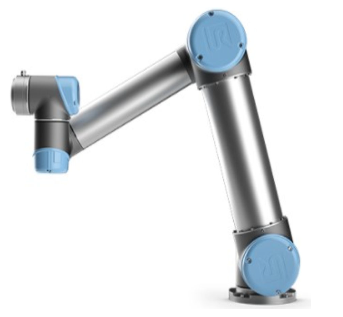
In order to verify the control performance of the proposed manipulator sliding mode controller, the control algorithm was simulated and verified on the MATLAB simulation platform and the virtual robot experimental platform CoppeliaSim. CoppeliaSim is a cross-platform robot dynamics simulation platform, which integrates several different physical engines and contains many different robot virtual physical models. The platform can simulate the robot very realistically, including the gravity, collision, and external force of the robot, and can highly restore the real application scenario of the robotic arm. On this platform, various physical simulation experiments can be done for different robots to verify the effectiveness of the control algorithm, which is convenient and practical and saves costs (https://www.coppeliarobotics.com/helpFiles/index.html) (accessed on 1 May 2022). In this paper, the 6-DOF UR5 manipulator in CoppeliaSim was used as the simulation object, and the remote API interface in CoppeliaSim was used to communicate with MATLAB to implement joint simulation. The physical simulation model of the UR5 manipulator is shown in Figure 2:

DH parameters of the UR5 manipulator are shown in

Table 1. DH parameters of the UR5 manipulator.

Joint	q (Rad)	d (m)	a (m)	$\mathit{\alpha }$ (Rad)
Joint1	$q_1$	0.089159	0	$\pi /2$
Joint2	$q_2$	0	−0.425	0
Joint3	$q_3$	0	−0.39225	0
Joint4	$q_4$	0.10915	0	$\pi /2$
Joint5	$q_5$	0.09465	0	$-\pi /2$
Joint6	$q_6$	0.0823	0	0

as follows:

The dynamic parameters of the UR5 manipulator are shown in

Table 2. Dynamic parameters of the UR5 manipulator.

Link	Mass (kg)	Center of Mass (m)
Link1	3.7	(0,−0.02561,0.00193)
Link2	8.393	(0.2125,0,0.11336)
Link3	2.33	(0.11993,0,0.0265)
Link4	1.219	(0,−0.0018,0.01634)
Link5	1.219	(0,0.0018,0.01634)
Link6	0.1879	(0,0,−0.001159)

as follows:

The motion range of each joint of the UR5 manipulator was set as $\left(-\pi ,\pi \right)$, and the initial joint angle was $\left(\pi /2,-8\pi /9,5\pi /6,0,\pi /2,0\right)$. The expected trajectory of the end of the UR5 manipulator was set in four groups: the first group was a uniform circular trajectory without considering the disturbance signal, the second group was a uniform circular trajectory considering the disturbance signal, the third group was a non-disturbing signal without considering the disturbance signal, and the fourth group was uniform square trajectory that do not consider disturbance signals. The four groups of trajectories were located on the x and z planes, and the coordinates in the y direction were fixed so that the manipulator only moved on the two-dimensional plane in the x and z directions. Through the inverse kinematics algorithm, the expected angles of each joint of the manipulator can be obtained.

To verify the performance of the manipulator sliding mode control algorithm (SMC-IERL) based on the improved exponential reaching law and nonlinear sliding mode surface for the trajectory tracking control of the end of the manipulator. We compare and analyze SMC-IERL with SMC-ERL and CTC, respectively.

(1)

Manipulator Control Algorithm Based on Computational Torque Method (CTC):

$$\mathit{\tau }=\mathit{M}(\mathit{q})({\ddot{\mathit{q}}}_{\mathit{d}}+K_p\mathit{e}+K_d\dot{\mathit{e}}+K_i\int \mathit{e}dt)+\mathit{C}(\mathit{q},\dot{\mathit{q}})\dot{\mathit{q}}+\mathit{G}(\mathit{q})-{\mathit{\tau }}_{\mathit{d}},$$

(33)

in (33), $K_P=100$, $K_d=2\sqrt{K_P}$, $K_i=1$. Using this relationship between $K_p$ and $K_i$, a decoupled closed-loop system can be realized; each joint response equaled the response of a critical damped linear second-order system [33]. The selection of the above parameters referred to the optimal parameters selected after many tests.

(2)

The traditional sliding mode control algorithm of manipulator based on exponential reaching law (SMC-ERL): The sliding surface selected by SMC-ERL was $\mathit{s}=\mathit{Ce}+\dot{\mathit{e}}$, the law of reaching was $\dot{\mathit{s}}=-{\mathit{K}}_{\mathbf{1}}\mathit{s}-{\mathit{K}}_{\mathbf{2}}sign\left(\mathit{s}\right)$, The controller was as follows (34):

$$\mathit{\tau }=\mathit{M}\left(\mathit{q}\right)({\ddot{\mathit{q}}}_{\mathit{d}}+{\mathit{K}}_{\mathbf{3}}\dot{\mathit{e}}+{\mathit{K}}_{\mathbf{1}}\mathit{s}+{\mathit{K}}_{\mathbf{2}}\mathit{sign}\left(\mathit{s}\right))+\mathit{C}(\mathit{q},\dot{\mathit{q}})\dot{\mathit{q}}+\mathit{G}\left(\mathit{q}\right)-{\mathit{\tau }}_{\mathit{d}},$$

(34)

in (34), ${\mathit{K}}_{\mathbf{3}}=[5;5;5;5;5;5]$, ${\mathit{K}}_{\mathbf{1}}=[20;20;20;20;20;20]$, ${\mathit{K}}_{\mathbf{2}}=[2;2;2;2;2;2]$. The selection of the above parameters referred to the optimal parameters selected after many tests.

(3)

Sliding mode control algorithm of manipulator based on improved reaching law and sliding surface (SMC-IERL): The selected sliding surface was a nonlinear sliding surface, as shown in (4). The selected reaching law was an improved exponential reaching law, as shown in (22) and (23). The selected controller was shown in (28). In (28), ${\mu }_1=1$, ${\mu }_2=3$, $m=7$, $p=5$, $k=5$, $l=7$, ${\mathit{K}}_{\mathbf{1}}=[20;20;20;20;20;20]$, ${\mathit{K}}_{\mathbf{2}}=[2;2;2;2;2;2]$, in (23), $\Delta =0.5$, $\alpha =4$, $\beta =1$. For fairness, some parameters of SMC-IERL were consistent with those of SMC-ERL.

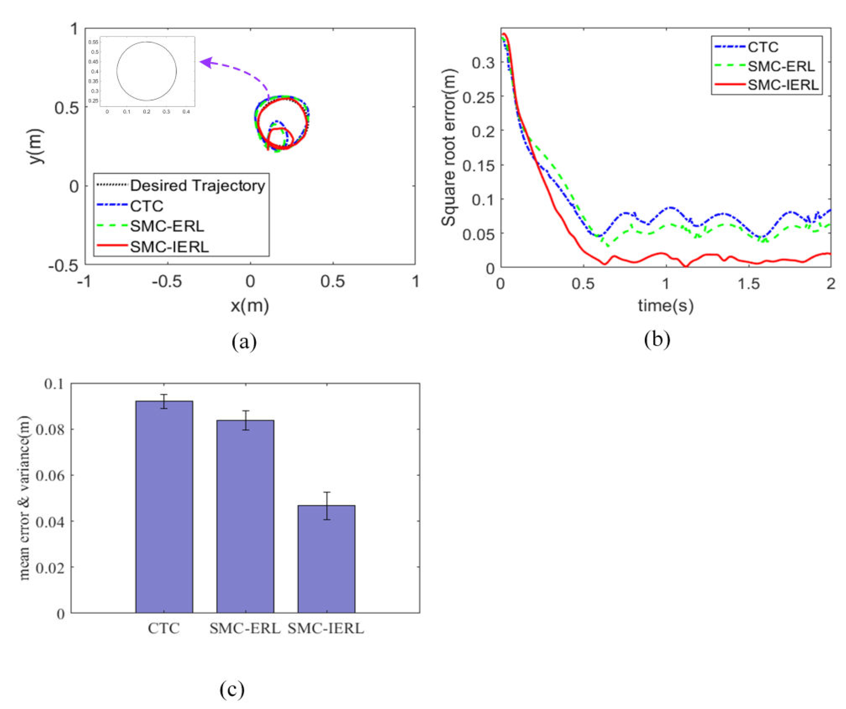
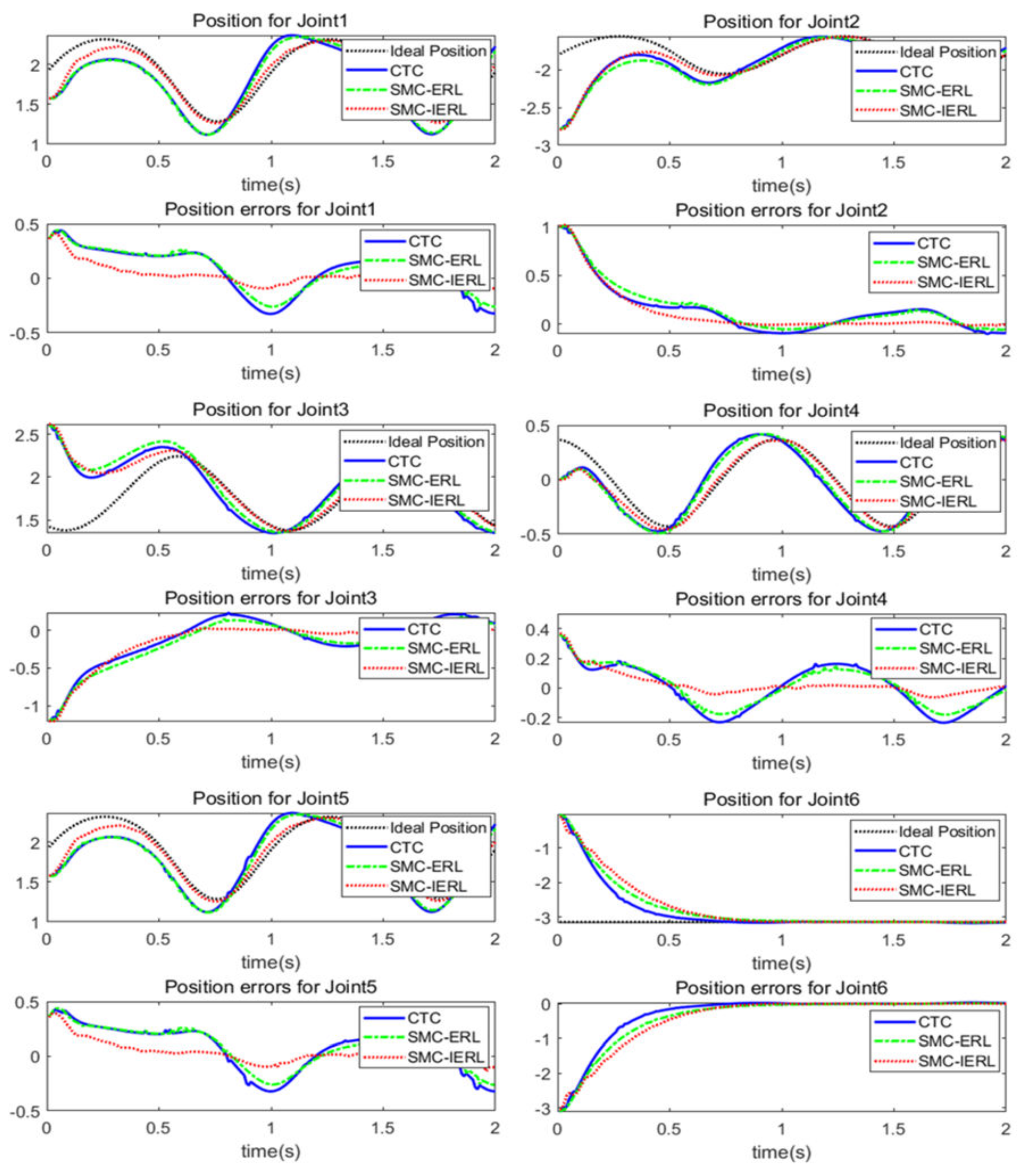
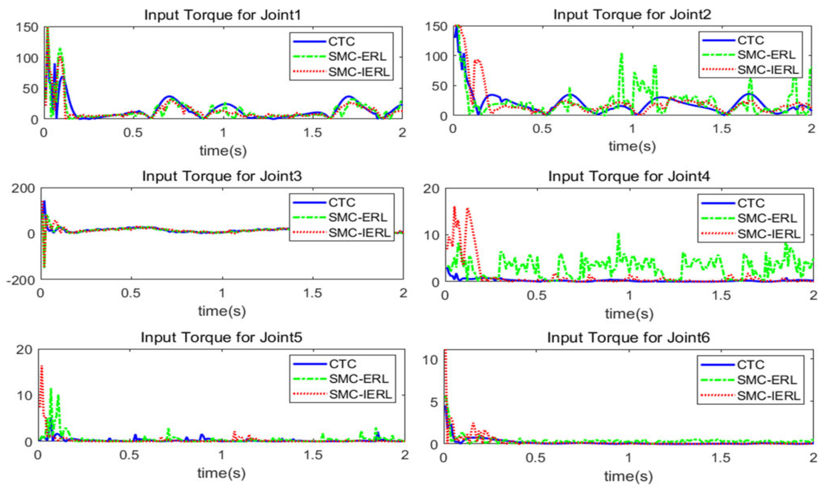
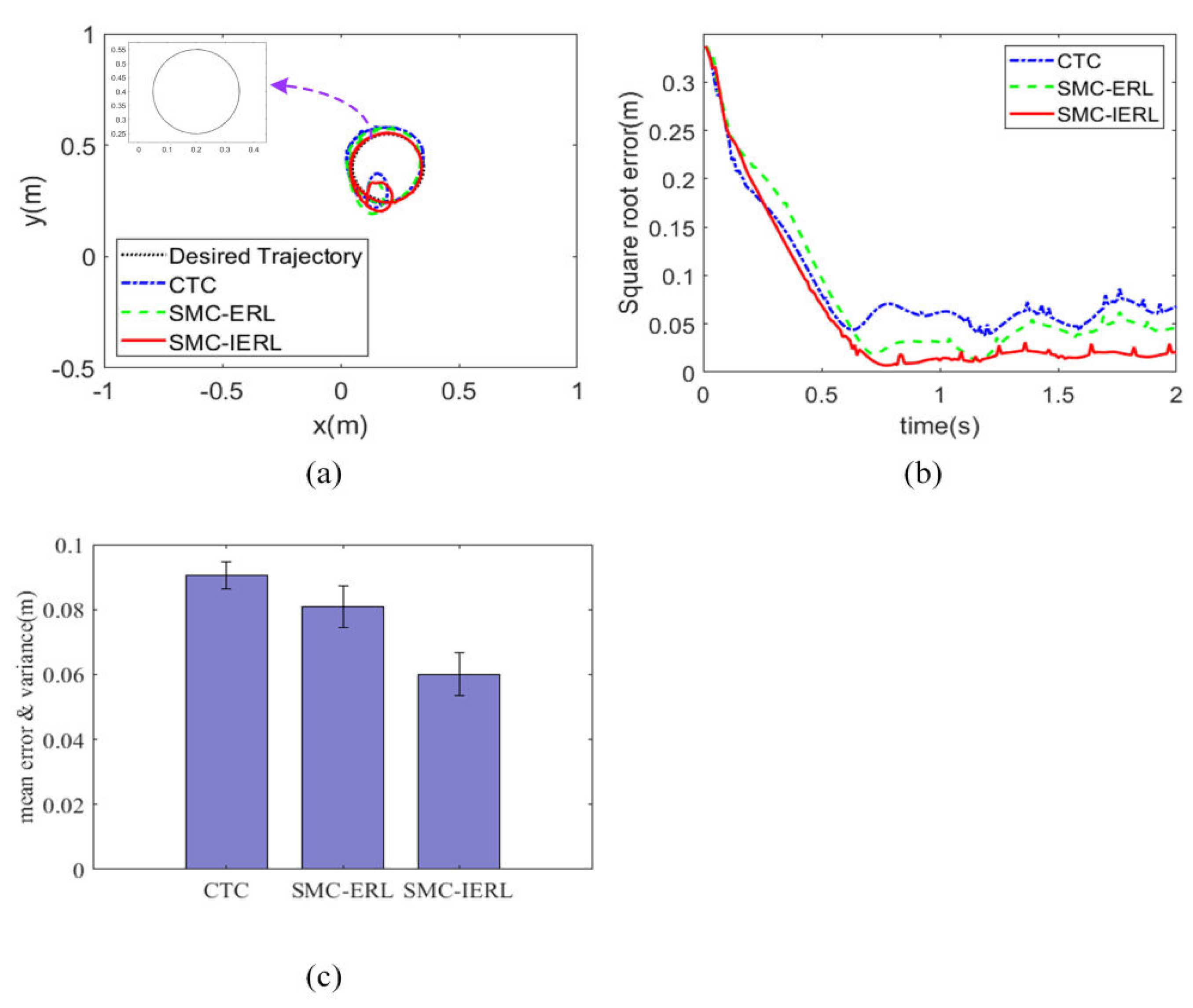
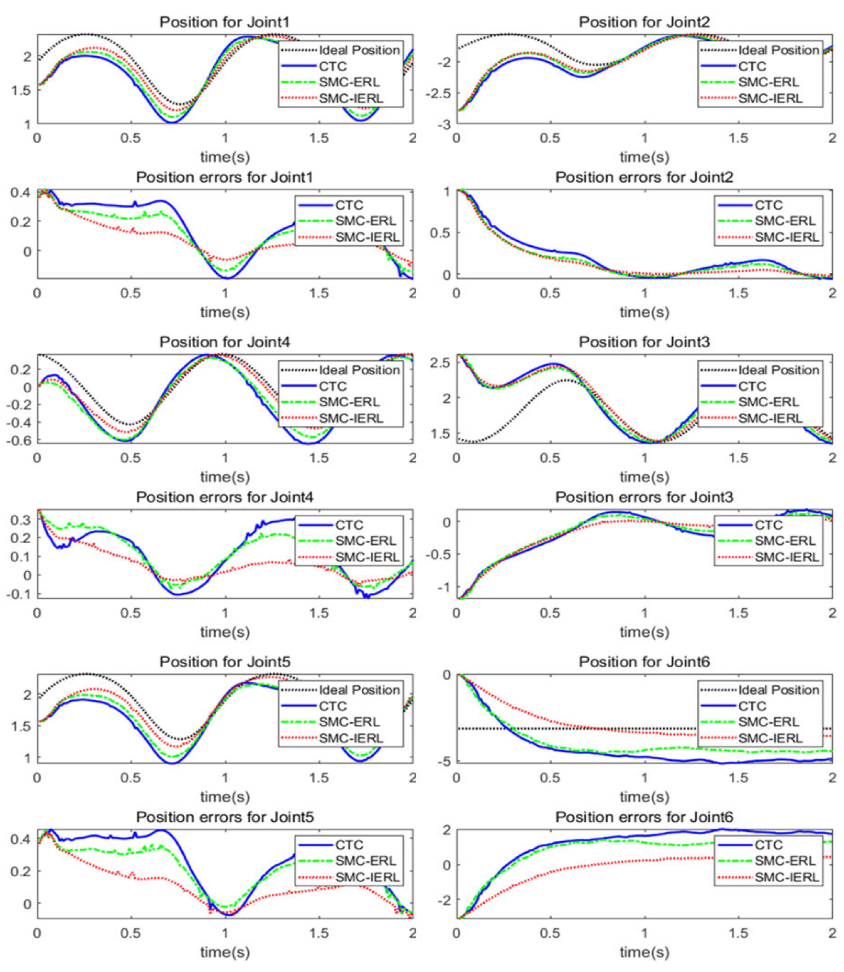
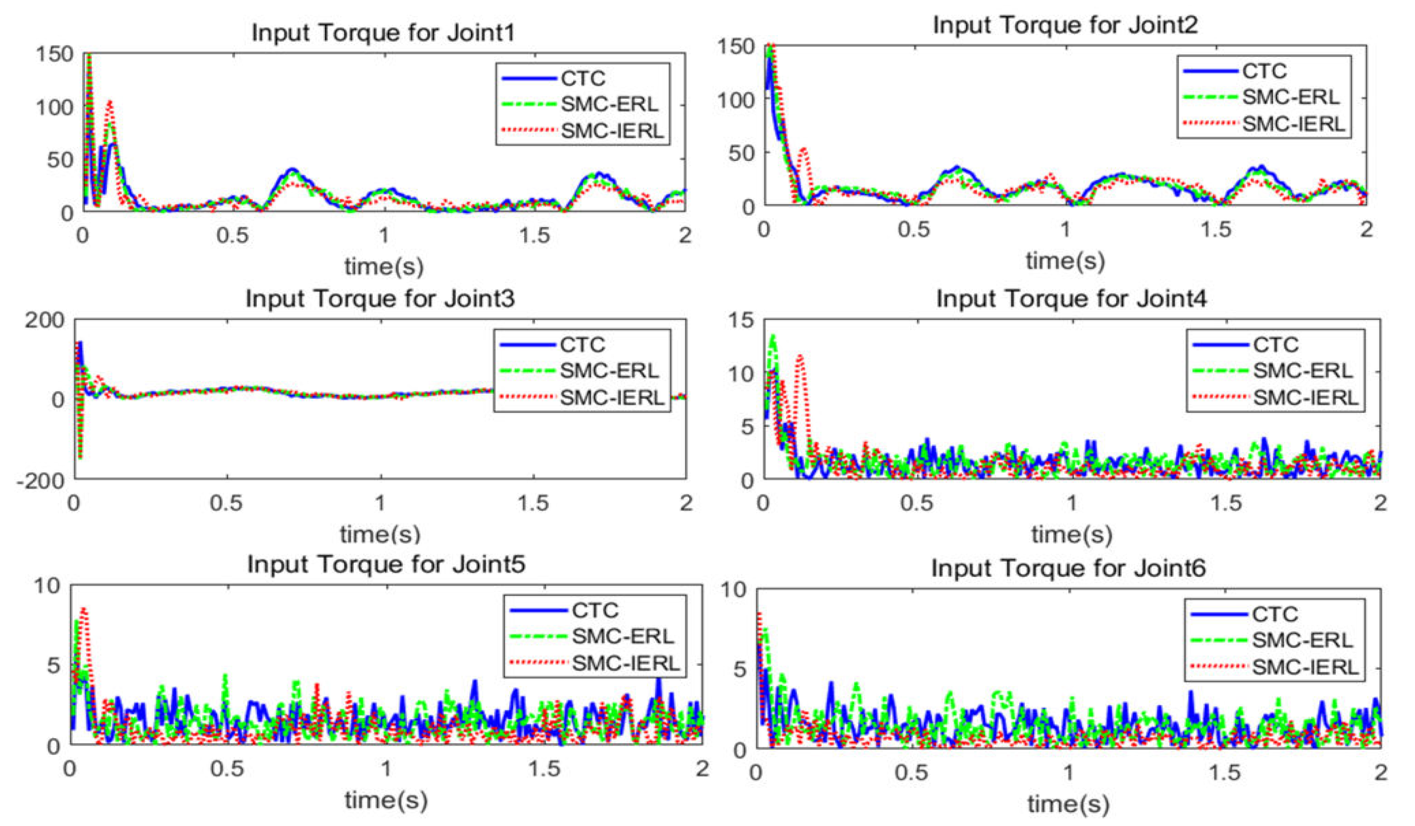
The first group of experiments used CTC, SMC-ERL, and SMC-IERL to track the desired uniform circular trajectory at the end of the UR5 manipulator without considering the disturbance signal, respectively. Figure 3a shows the trajectory tracking diagrams of the desired uniform circular trajectory and the three control algorithms of CTC, SMC-ERL, and SMC-IRL. Figure 3b is the square root error comparison of CTC, SMC-ERL, and SMC-IERL. Figure 3c is the comparison of mean error and variance among CTC, SMC-ERL, and SMC-IERL. Figure 4 shows the expected position of each joint and the position of each joint obtained by tracking the uniform circular trajectory according to the three control algorithms, and the error comparison between the position of each joint and the expected position of each joint. Figure 5 shows the comparison of the output torques of each joint obtained by the three control algorithms tracking the uniform circular trajectory.

The second group of experiments used CTC, SMC-ERL, and SMC-IERL to track the desired uniform circular trajectory at the end of the UR5 manipulator under the condition of considering the disturbance signal. Among them, the disturbance signal was set as ${\mathit{\tau }}_{\mathit{d}}=0.5rand(6,1)$, $rand(6,1)$ means to generate random values in the range of [0∼1] with 6 rows and 1 column, which satisfy the normal distribution. The purpose of adding a disturbance signal was to verify the robustness and feasibility of the proposed control scheme SMC-IERL, which can simulate the actual manipulator system more realistically. Figure 6a is the trajectory tracking diagram of the expected uniform circular trajectory and the three control algorithms of CTC, SMC-ERL, and SMC-IERL. Figure 6b is the square root error comparison of CTC, SMC-ERL, and SMC-IERL. Figure 6c is the comparison of mean error and variance among CTC, SMC-ERL, and SMC-IERL. Figure 7 shows the expected position of each joint and the position of each joint obtained by tracking the uniform circular trajectory according to the three control algorithms, and the error comparison between the position of each joint and the expected position of each joint with considering the disturbance signal. Figure 8 shows the comparison of the output torques of each joint obtained by the three control algorithms tracking the uniform circular trajectory.

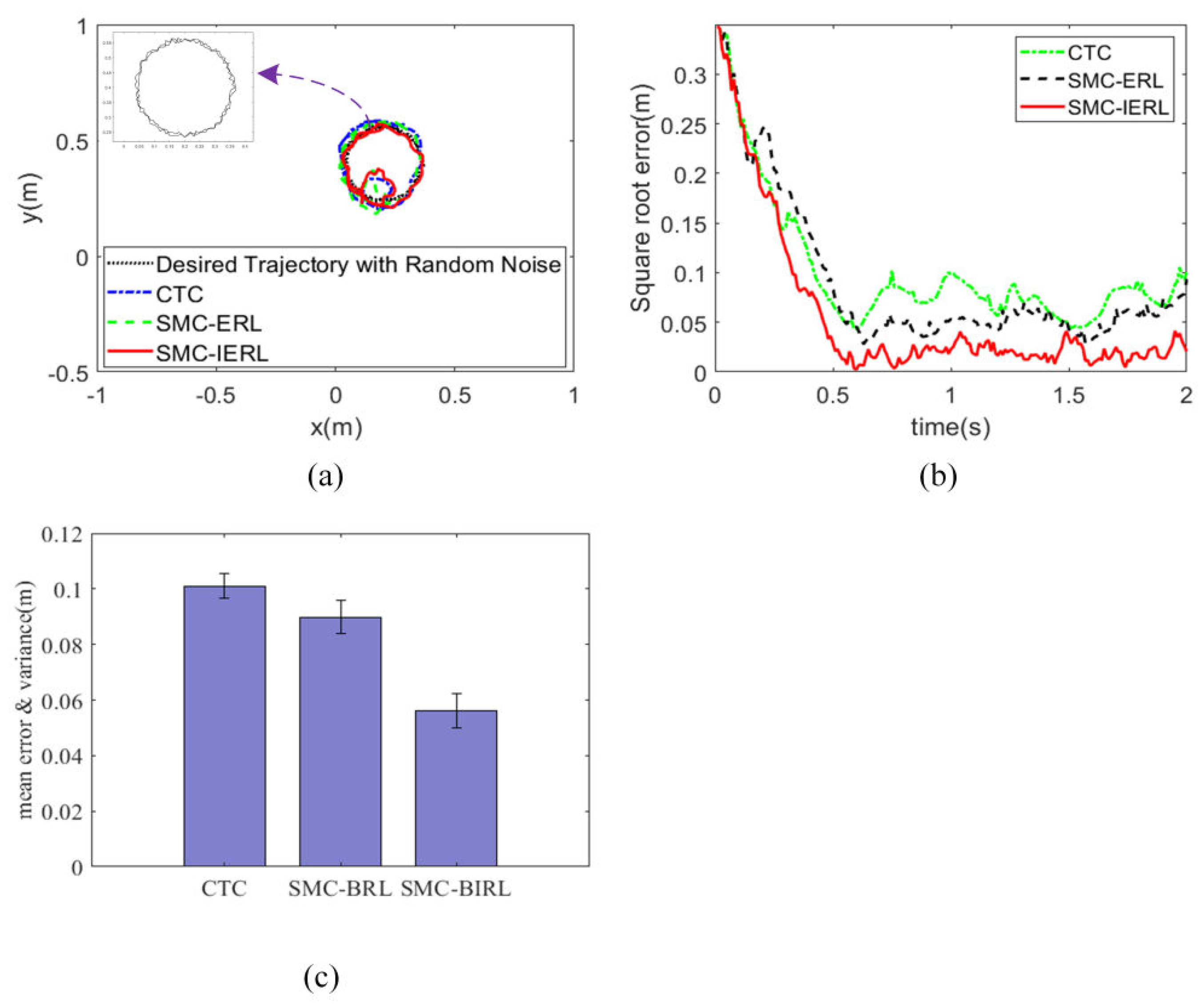
In the third group, CTC, SMC-ERL, and SMC-IERL were used to track the desired non-uniform circular trajectory at the end of the UR5 manipulator without considering the disturbance signal, respectively. The non-uniform circular trajectory was set to introduce random signals [0∼0.02] on the radius of the uniform circular trajectory. Figure 9a is the trajectory tracking diagram of expected non-uniform circular trajectory and CTC, SMC-ERL, and SMC-IERL three control algorithms; Figure 9b is the square root error comparison of CTC, SMC-ERL, and SMC-IERL. Figure 9c is the comparison of mean error and variance among CTC, SMC-ERL, and SMC-IERL. Figure 10 shows the expected position of each joint and the position of each joint obtained by tracking the non-uniform circular trajectory according to the three control algorithms, and the error comparison between the position of each joint and the expected position of each joint without considering the disturbance signal. Figure 11 is the comparison of the output torque of each joint obtained by tracking the non-uniform circular trajectory of the three control algorithms.

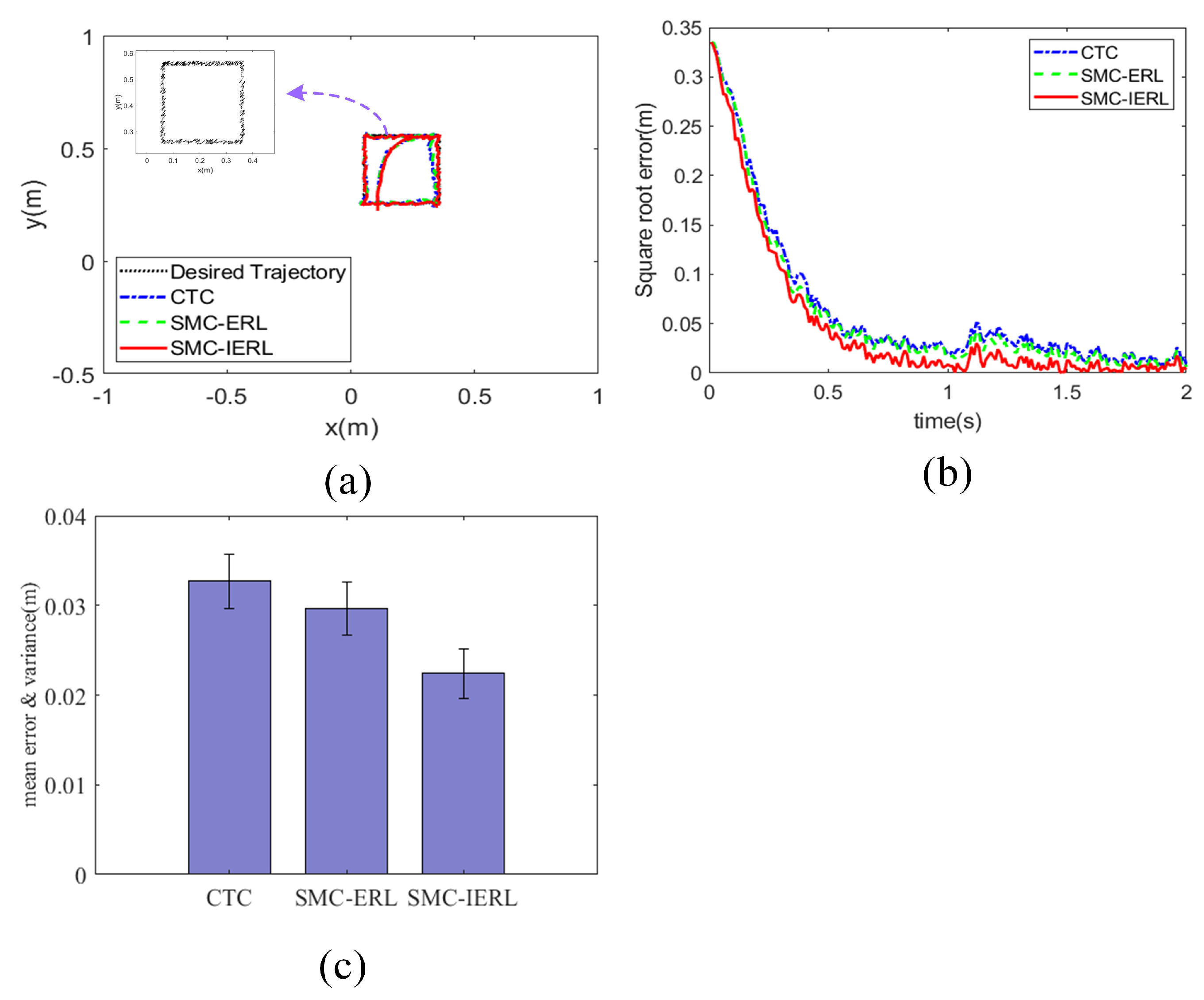
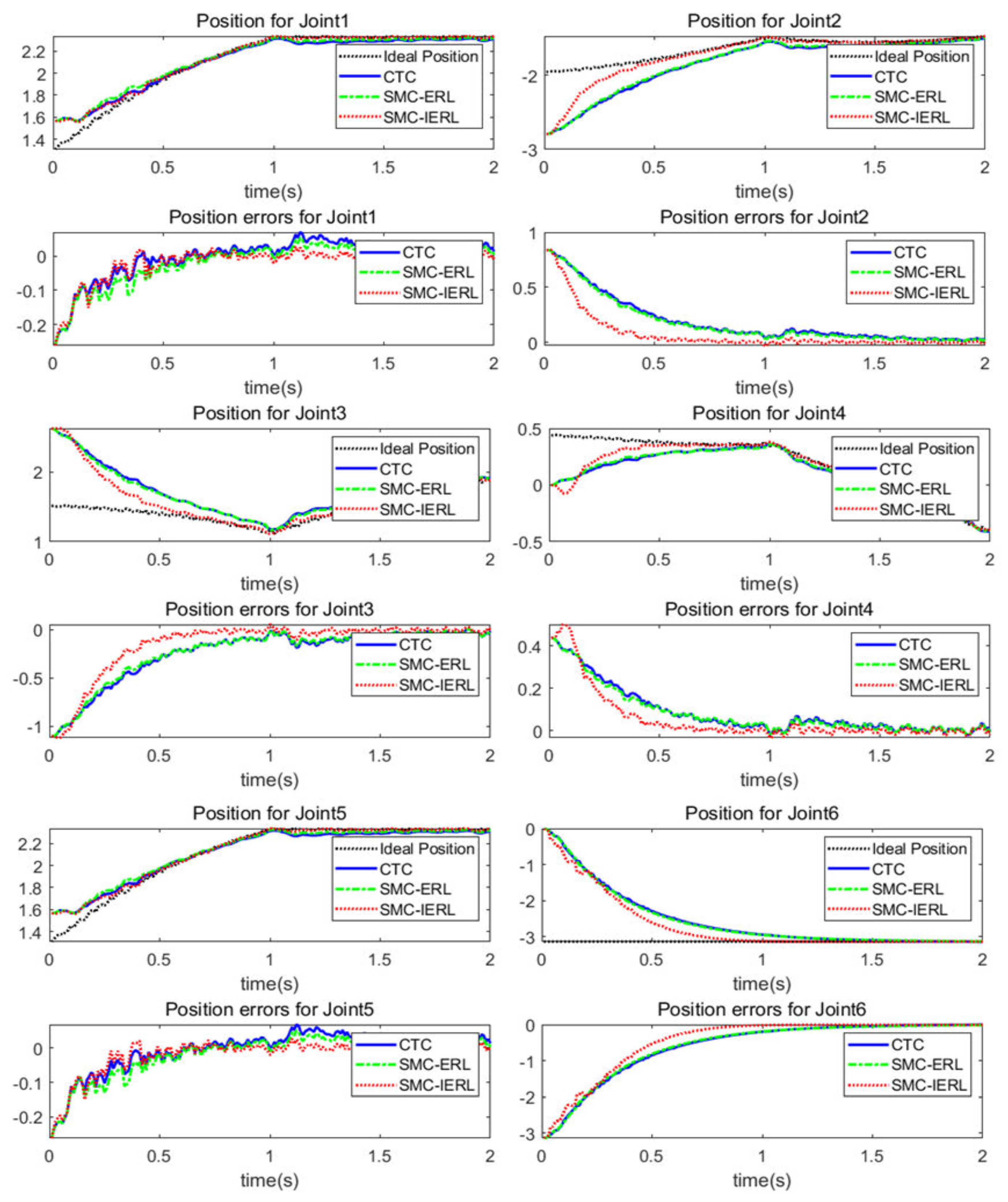
The fourth group of experiments used CTC, SMC-ERL, and SMC-IERL to track the desired non-uniform square trajectory at the end of the UR5 manipulator without considering the disturbance signal, respectively. The non-uniform square trajectory was set to introduce random signals [0∼0.02] on the uniform square trajectory. Figure 12a shows the trajectory tracking diagrams of the desired non-uniform square trajectory and the three control algorithms of CTC, SMC-ERL, and SMC-IRL. Figure 12b is the square root error comparison of CTC, SMC-ERL, and SMC-IERL. Figure 12c is the comparison of mean error and variance among CTC, SMC-ERL, and SMC-IERL. Figure 13 shows the expected position of each joint and the position of each joint obtained by tracking the non-uniform square trajectory according to the three control algorithms, and the error comparison between the position of each joint and the expected position of each joint without considering the disturbance signal. Figure 14 shows the comparison of the output torques of each joint obtained by the three control algorithms tracking the non-uniform square trajectory.

Without considering the disturbance signal, from Figure 3a, it can be seen intuitively that the three control algorithms can track the expected uniform circular trajectory. However, compared with CTC and SMC-ERL, SMC-IERL has the best tracking effect, which is most consistent with the expected uniform circular trajectory. From Figure 3b,c, it can be seen that SMC-IERL has the smallest square root error, mean error, and variance compared with CTC and SMC-ERL. In the early stage of tracking, it can quickly reduce the tracking error of the system, and the tracking performance is the best and the accuracy is the highest. It can be seen from Figure 4 that, when tracking the desired joints of each joint, the three control algorithms can effectively track the desired joints, but there are more or less tracking errors. Considering the position error of each joint and the convergence speed, CTC has the worst tracking accuracy and the slowest convergence speed. SMC-ERL has higher tracking accuracy than CTC, but the convergence speed has little difference from CTC. Compared with CTC and SMC-ERL, SMC-IERL can keep the error between the expected trajectory and the real trajectory in a relatively small range. The tracking accuracy of each joint is the highest, the convergence speed is the fastest, and the tracking performance is the best. It can be seen from Figure 5 that the SMC-ERL control scheme has a high-frequency chattering phenomenon on the output torque of joints 4 and 5, which seriously affects the control of the real manipulator system, and even makes the manipulators. There is loss of control and damage to the manipulators. Compared with SMC-ERL, CTC and SMC-IERL can weaken the chattering of the system to a certain extent. Considering the impact of the entire manipulator’s system control, SMC-IERL can better weaken the chattering of the output torque of each joint and has better robustness that is extremely important for the stability of the entire manipulator control system.

In the case of considering the disturbance signal, from Figure 5a, it can be seen intuitively that, when considering the disturbance signal, all three control algorithms can track the desired uniform circular trajectory, but compared with CTC, SMC-ERL, and SMC-IERL.The tracking works best and best matches the desired uniform circular trajectory. From Figure 6b,c, it can be seen that SMC-IERL has the smallest square root error, mean error, and variance than CTC and SMC-ERL. The system tracking error can be reduced in a very short period in the early stage of tracking, and the tracking performance is optimal and the accuracy is the highest. It can be seen from Figure 7 that, when tracking the desired joints of each joint, the three control algorithms can effectively track each desired joint, but there will be some tracking errors more or less. Considering the position error and convergence speed of each joint, CTC has the worst tracking accuracy and the slowest convergence speed. Compared with CTC, SMC-ERL has a certain degree of improvement in tracking accuracy, but the convergence speed is not much different from CTC. Compared with CTC and SMC-ERL, SMC-IERL can keep the error between the expected trajectory and the real trajectory in a relatively small range. The tracking accuracy of each joint is the highest, the convergence speed is the fastest, and the tracking performance is the best. It can be seen from Figure 8 that, in the control of joints 4, 5, and 6, both CTC and SMC-ERL have a high-frequency chattering phenomenon, and the proposed SMC-IERL control scheme is compared with CTC. SMC-ERL can effectively weaken the chattering phenomenon of joints 4, 5, and 6. Considering the control of the entire manipulator system, SMC-IERL shows better control performance and better robustness.

Without considering the disturbance signal, from Figure 9a, all three control algorithms can track the expected non-uniform circular trajectory, but, compared with CTC and SMC-ERL, SMC-IERL has the best tracking effect, which is similar to the expected non-uniform circular trajectory. It can be seen from Figure 9b,c that, among the three control algorithms, SMC-IERL has the smallest square root error, mean error, and variance. In the early stage of tracking, SMC-IERL can quickly reduce the system tracking error, with strong rapidity, the highest tracking accuracy, and the best tracking performance. It can be seen from Figure 10 that CTC has a large error fluctuation range when tracking the desired joint positions, especially for the tracking of the desired joint positions of joint 1, joint 4, and joint 5. Next to SMC-ERL, SMC-IERL has the smallest error fluctuation and can keep the error range at a relatively small level. Considering the position error and convergence speed of each joint, CTC has the worst tracking accuracy and the slowest convergence speed. Compared with CTC, SMC-ERL has a certain degree of improvement in tracking accuracy, but the convergence speed is not very different from CTC. Compared with CTC and SMC-ERL, SMC-IERL has the highest tracking accuracy for each joint and has the fastest convergence speed and the best tracking performance. It can be seen from the output torque of each joint in Figure 11 that, when the given expected trajectory is an uneven circular trajectory with random signals, both CTC and SMC-ERL have a high-frequency chattering phenomenon, which is extremely difficult to control the real manipulator system. Compared with CTC, SMC-ERL and SMC-IERL weaken the chattering of the control system to a large extent and shows better robustness. For artificially given non-uniform circular trajectories with random signals, SMC-IERL can still track quickly and stably and has good robustness, which also shows from the side that SMC-IERL has a certain universality.

Without considering the disturbance signal, it can be seen intuitively from Figure 12a that the three control algorithms can track the desired non-uniform square trajectory. Compared with CTC and SMC-ERL, SMC-IERL has the best tracking effect and the most overlap with the expected uniform square trajectory. It can be seen from Figure 12b,c that SMC-IERL has the smallest square root error, mean error, and variance, and the highest tracking accuracy compared with CTC and SMC-ERL. It can be seen from Figure 13 that, when tracking the desired joints of each joint, the three control algorithms can effectively track the desired joints, but there are more or less tracking errors. Considering the position error and convergence speed of each joint, SMC-ERL has the worst tracking accuracy and the slowest convergence speed. SMC-IERL and CTC can quickly converge the tracking error to a relatively small range until zero. From Figure 14, it can be seen that the SMC-ERL control scheme has a high-frequency chattering phenomenon on the output torque of joints 2, 4, and 5, which seriously affects the control of the real manipulator system. Compared with SMC-ERL and CTC, SMC-IERL reduces the chattering of the system to some extent under the condition of ensuring the robustness, stability, and control accuracy of the system.

5. Conclusions

In this paper, an improved exponential reaching law and nonlinear sliding mode surface are proposed for the convergence speed and chattering problem in the sliding mode variable structure control of the manipulator, and the Lyapunov function is used to analyze its stability. The trajectory tracking simulation experiment of the manipulator end is carried out on the simulation experiment platform to verify the tracking performance of the proposed control scheme. The simulation results show that the proposed control scheme (SMC-IERL) can guarantee the fast convergence of the system and weaken the chattering ability of the system under the premise of ensuring the robustness of the system when tracking different expected trajectories. Even in the presence of a disturbance signal, it can still ensure the robustness and control accuracy of the system. By comparing SMC-IERL with CTC and SMC-ERL, the control performance and advantages of SMC-IERL on the basis of ensuring system stability and robustness are verified. Based on the research in this paper, our follow-up research work considers continuing to study different reaching laws and sliding surfaces to design controllers. At the same time, we consider using various optimization algorithms to optimize the parameters of our proposed controller, including but not limited to genetic algorithms and neural network algorithms.

References

- Rocco, P. Stability of PID control for industrial robot arms. IEEE Trans. Robot. Autom. 1996, 12, 606–614. [Google Scholar] [CrossRef] [Green Version]
- Aguilar-Ibanez, C.; Moreno-Valenzuela, J.; García-Alarcón, O.; Martinez-Lopez, M.; Acosta, J.Á.; Suarez-Castanon, M.S. PI-Type Controllers and Σ–Δ Modulation for Saturated DC-DC Buck Power Converters. IEEE Access 2021, 9, 20346–20357. [Google Scholar] [CrossRef]
- Soriano, L.A.; Zamora, E.; Vazquez-Nicolas, J.; Hernández, G.; Barraza Madrigal, J.A.; Balderas, D. PD control compensation based on a cascade neural network applied to a robot manipulator. Front. Neurorobotics 2020, 14, 78. [Google Scholar] [CrossRef] [PubMed]
- Silva-Ortigoza, R.; Hernández-Márquez, E.; Roldán-Caballero, A.; Tavera-Mosqueda, S.; Marciano-Melchor, M.; García-Sánchez, J.R.; Hernández-Guzmán, V.M.; Silva-Ortigoza, G. Sensorless Tracking Control for a “Full-Bridge Buck Inverter–DC Motor” System: Passivity and Flatness-Based Design. IEEE Access 2021, 9, 132191–132204. [Google Scholar] [CrossRef]
- Liu, M. Decentralized control of robot manipulators: Nonlinear and adaptive approaches. IEEE Trans. Autom. Control 1999, 44, 357–363. [Google Scholar]
- Hu, Q.; Xu, L.; Zhang, A. Adaptive backstepping trajectory tracking control of robot manipulator. J. Frankl. Inst. 2012, 349, 1087–1105. [Google Scholar] [CrossRef]
- Kali, Y.; Saad, M.; Benjelloun, K. Optimal super-twisting algorithm with time delay estimation for robot manipulators based on feedback linearization. Robot. Auton. Syst. 2018, 108, 87–99. [Google Scholar] [CrossRef]
- Islam, S.; Liu, X.P. Robust sliding mode control for robot manipulators. IEEE Trans. Ind. Electron. 2010, 58, 2444–2453. [Google Scholar] [CrossRef]
- Balcazar, R.; Rubio, J.d.J.; Orozco, E.; Andres Cordova, D.; Ochoa, G.; Garcia, E.; Pacheco, J.; Gutierrez, G.J.; Mujica-Vargas, D.; Aguilar-Ibañez, C. The Regulation of an Electric Oven and an Inverted Pendulum. Symmetry 2022, 14, 759. [Google Scholar] [CrossRef]
- de Jesús Rubio, J.; Orozco, E.; Cordova, D.A.; Islas, M.A.; Pacheco, J.; Gutierrez, G.J.; Zacarias, A.; Soriano, L.A.; Meda-Campaña, J.A.; Mujica-Vargas, D. Modified Linear Technique for the Controllability and Observability of Robotic Arms. IEEE Access 2022, 22, 3366–3377. [Google Scholar] [CrossRef]
- Soriano, L.A.; Rubio, J.d.J.; Orozco, E.; Cordova, D.A.; Ochoa, G.; Balcazar, R.; Cruz, D.R.; Meda-Campaña, J.A.; Zacarias, A.; Gutierrez, G.J. Optimization of Sliding Mode Control to Save Energy in a SCARA Robot. Mathematics 2021, 9, 3160. [Google Scholar] [CrossRef]
- Wang, F.; Chao, Z.Q.; Huang, L.B.; Li, H.Y.; Zhang, C.Q. Trajectory tracking control of robot manipulator based on RBF neural network and fuzzy sliding mode. Clust. Comput. 2019, 22, 5799–5809. [Google Scholar] [CrossRef]
- Bouakrif, F.; Zasadzinski, M. Trajectory tracking control for perturbed robot manipulators using iterative learning method. Int. J. Adv. Manuf. Technol. 2016, 87, 2013–2022. [Google Scholar] [CrossRef]
- Ji, P.; Ma, F.; Min, F. Terminal Traction Control of Teleoperation Manipulator With Random Jitter Disturbance Based on Active Disturbance Rejection Sliding Mode Control. IEEE Access 2020, 8, 220246–220262. [Google Scholar] [CrossRef]
- Tsai, H.H.; Fuh, C.C.; Ho, J.R.; Lin, C.K.; Tung, P.C. Controller Design for Unstable Time-Delay Systems with Unknown Transfer Functions. Mathematics 2022, 10, 431. [Google Scholar] [CrossRef]
- Danik, Y.; Dmitriev, M. Symbolic Regulator Sets for a Weakly Nonlinear Discrete Control System with a Small Step. Mathematics 2022, 10, 487. [Google Scholar] [CrossRef]
- Tian, X.; Yang, Z. Adaptive stabilization of a fractional-order system with unknown disturbance and nonlinear input via a backstepping control technique. Symmetry 2019, 12, 55. [Google Scholar] [CrossRef] [Green Version]
- Shi, B.; Wu, H.; Zhu, Y.; Shang, M. Robust Control of a New Asymmetric Teleoperation Robot Based on a State Observer. Sensors 2021, 21, 6197. [Google Scholar] [CrossRef] [PubMed]
- Gu, Y.; Li, Z.; Zhang, Z.; Li, J.; Chen, L. Path tracking control of field information-collecting robot based on improved convolutional neural network algorithm. Sensors 2020, 20, 797. [Google Scholar] [CrossRef] [PubMed] [Green Version]
- Nguyen, L.V.; Phung, M.D.; Ha, Q.P. Iterative Learning Sliding Mode Control for UAV Trajectory Tracking. Electronics 2021, 10, 2474. [Google Scholar] [CrossRef]
- Slotine, J.J.; Sastry, S.S. Tracking control of nonlinear systems using sliding surfaces, with application to robot manipulators. Int. J. Control 1983, 38, 465–492. [Google Scholar] [CrossRef] [Green Version]
- Zhihong, M.; Paplinski, A.P.; Wu, H.R. A robust MIMO terminal sliding mode control scheme for rigid robotic manipulators. IEEE Trans. Autom. Control 1994, 39, 2464–2469. [Google Scholar] [CrossRef]
- Feng, Y.; Yu, X.; Man, Z. Non-singular terminal sliding mode control of rigid manipulators. Automatica 2002, 38, 2159–2167. [Google Scholar] [CrossRef]
- Gao, W.; Hung, J.C. Variable structure control of nonlinear systems: A new approach. IEEE Trans. Ind. Electron. 1993, 40, 45–55. [Google Scholar]
- Hong, M.; Yong, W. Fast convergent sliding mode variable structure control of robot. Inf. Control 2009, 38, 552–557. [Google Scholar]
- Fallaha, C.J.; Saad, M.; Kanaan, H.Y.; Al-Haddad, K. Sliding-mode robot control with exponential reaching law. IEEE Trans. Ind. Electron. 2010, 58, 600–610. [Google Scholar] [CrossRef]
- Ma, H.; Wu, J.; Xiong, Z. A novel exponential reaching law of discrete-time sliding-mode control. IEEE Trans. Ind. Electron. 2017, 64, 3840–3850. [Google Scholar] [CrossRef]
- Lam, N.T.; Nguyen, H.Q.; Duong, M.D.; Ngo, K.T. Exponential reaching law sliding mode control for dual arm robots. J. Eng. Sci. Technol. 2020, 15, 2841–2853. [Google Scholar]
- Devika, K.; Thomas, S. Improved sliding mode controller performance through power rate exponential reaching law. In Proceedings of the 2017 Second International Conference on Electrical, Computer and Communication Technologies (ICECCT), Coimbatore, Tamil Nadu, India, 22–24 February 2017; IEEE: Piscataway, NJ, USA, 2017; pp. 1–7. [Google Scholar]
- Wang, J.; Lee, M.C.; Kim, J.H.; Kim, H.H. Fast fractional-order terminal sliding mode control for seven-axis robot manipulator. Appl. Sci. 2020, 10, 7757. [Google Scholar] [CrossRef]
- Wu, Y.D.; Wu, S.F.; Gong, D.R.; Kang, Z.Y.; Wang, X.L. Spacecraft Attitude Maneuver Using Fast Terminal Sliding Mode Control Based on Variable Exponential Reaching Law. In Proceedings of the International Conference on Aerospace System Science and Engineering, Toronto, ON, Canada, 30 July–1 August 2019; Springer: Berlin/Heidelberg, Germany, 2019; pp. 1–10. [Google Scholar]
- Zhang, J.; Liu, B.; Jiang, Z.; Hu, H. The application of sliding mode control with improved approaching law in manipulator control. In Proceedings of the 2018 13th IEEE Conference on Industrial Electronics and Applications (ICIEA), Wuhan, China, 31 May–2 June 2018; IEEE: Piscataway, NJ, USA, 2018; pp. 807–812. [Google Scholar]
- Sangdani, M.; Tavakolpour-Saleh, A.R.; Lotfavar, A. Genetic algorithm-based optimal computed torque control of a vision-based tracker robot: Simulation and experiment. Eng. Appl. Artif. Intell. 2018, 67, 24–38. [Google Scholar] [CrossRef]
Figure 1.
Schematic diagram of the sliding mode control system of the manipulator.
Figure 2.
Physical simulation model of the UR5 manipulator.
Figure 3.
Uniform circular trajectory tracking experiment without considering disturbance signal. (a) comparison of trajectory tracking for desired uniform circular trajectory with three control algorithms; (b) comparison of square root error of three control algorithms; (c) comparison of mean error and variance of three control algorithms.
Figure 4.
In the uniform circular trajectory experiment without considering disturbance signal, the expected position of each joint is compared with the position and error of each joint obtained by the three control algorithms.
Figure 5.
In the uniform circular trajectory experiment without considering disturbance signal, the output torque of each joint obtained by the three control algorithms is compared.
Figure 6.
Uniform circular trajectory tracking experiment with disturbance signal. (a) comparison of trajectory tracking for desired uniform circular trajectory with three control algorithms; (b) comparison of square root error of three control algorithms; (c) comparison of mean error and variance of three control algorithms.
Figure 7.
In the uniform circular trajectory experiment with disturbance signal, the expected position of each joint is compared with the position and error of each joint obtained by the three control algorithms.
Figure 8.
In the uniform circular trajectory experiment with disturbance signal, the output torque of each joint obtained by the three control algorithms is compared.
Figure 9.
Non-uniform circular trajectory tracking experiment without considering disturbance signal. (a) comparison of trajectory tracking for desired non-uniform circular trajectory with three control algorithms; (b) comparison of square root error of three control algorithms; (c) comparison of mean error and variance of three control algorithms.
Figure 10.
In the non-uniform circular trajectory experiment without considering disturbance signal, the expected position of each joint is compared with the position and error of each joint obtained by the three control algorithms.
Figure 11.
In the non-uniform circular trajectory experiment without considering disturbance signal, the output torque of each joint obtained by the three control algorithms is compared.
Figure 12.
Non-uniform square trajectory tracking experiment without considering disturbance signal. (a) comparison of trajectory tracking for desired non-uniform square trajectory with three control algorithms; (b) comparison of square root error of three control algorithms; (c) comparison of mean error and variance of three control algorithms.
Figure 13.
In the non-uniform square trajectory experiment without considering disturbance signal, the expected position of each joint is compared with the position and error of each joint obtained by the three control algorithms.
Figure 14.
In the non-uniform square trajectory experiment without considering disturbance signal, the output torque of each joint obtained by the three control algorithms is compared.