A Note on the Laguerre-Type Appell and Hypergeometric Polynomials

Abstract

The Laguerre derivative and its iterations have been used to define new sets of special functions, showing the possibility of generating a kind of parallel universe for mathematical entities of this kind. In this paper, we introduce the Laguerre-type Appell polynomials, in particular, the Bernoulli and Euler case, and we examine a set of hypergeometric Laguerre–Bernoulli polynomials. We show their main properties and indicate their possible extensions.

1. Introduction

Special functions and special number sequences are not only interesting from a theoretical point of view, but are also widely used in physical applications (electrodynamics, classical mechanics and quantum mechanics), engineering and applied mathematics, life sciences and many other fields of science. The vast majority of special functions, including elliptic integrals, beta functions, the incomplete gamma function, Bessel functions, Legendre functions, classic orthogonal polynomials, Kummer confluent functions, etc., are represented in terms of hypergeometric functions, through the introduction of suitable parameters. Many multivariate generalizations of hypergeometric functions have been studied in the literature, including via an extension of the Pochhammer symbol [1,2,3,4,5,6,7,8,9].

In the field of polynomial functions, the literature on Bernoulli polynomials and numbers is vast [10], since they frequently appear in mathematics. Along with the Stiring numbers, they play a central role in number theory. The Bernoulli numbers arose from the process of summing powers of integers; however, this sequence of numbers occurs surprisingly often in many areas of mathematics, such as the Taylor expansion in a neighborhood of the origin of circular and hyperbolic tangent and cotangent functions, and the residual term of the Euler–MacLaurin quadrature rule. Furthermore, there are intimate connections with the Riemann zeta function and even with Fermat’s last theorem.

As D.E. Smith noted [11], among all the sequences of numbers “there is hardly a species so important and so generally applicable as Bernoulli numbers”.

Generalizations of the classical Bernoulli polynomials were previously considered in [12,13,14,15]. The hypergeometric Bernoulli polynomials have been introduced and recently studied in several articles [16,17,18,19,20], in connection with generalizations of the Riemann Zeta function [21,22,23,24].

In this paper, recalling the Laguerre-type derivative and the possibility of constructing special functions generated by the corresponding differential isomorphism (see [25] and the references therein), we examine the case of the Laguerre-type Appell polynomials and consider, in particular, their extensions to the case of hypergeometric Bernoulli polynomials, restricting ourselves to the case of the first-order Laguerre derivative.

It is worth noting that several applications have been implemented using the Laguerre derivative, in connection with population dynamics [25].

In Section 2 we recall the Laguerre-type exponentials and the differential isomorphism producing the relevant special functions. Then we consider, in particular, the case of Laguerre-type Appell polynomials (Section 3), including the Bernoulli and Euler cases.

Lastly, in Section 4, we introduce the Laguerre-type hypergeometric polynomials, considering only the simplest cases, that is, for $k=1$ and $k=2$.

Of course, several further extensions could be made, considering higher values of k, or iterating the isomorphism described in [26] to higher-order Laguerre derivatives, as is recalled in the Conclusions, but this provides no further information, since the methodology remains essentially the same.

2. Laguerre-Type Exponentials and Special Functions

The Laguerre derivative, is defined by

$$\begin{array}{c}\hfill D_L:=DxD=D+x{D}^2,\end{array}$$

(1)

where $D=D_x=d/dx$. In [25] it is shown that, for all complex numbers a, it results in:

$$\begin{array}{c}\hfill D_L{e}_1\left(ax\right)=a{e}_1\left(ax\right),\end{array}$$

(2)

where $e_1\left(x\right)={\sum }_{k=0}^{\infty }{x}^k/{(k!)}^2$ is the first-order Laguerre-type exponential [27,28].

The above property can be iterated when, defining Laguerre-type exponentials of higher order, called L-exponentials. In general, (see [28], Theorem 2.2).

Theorem 1.

The function

$$\begin{array}{c}\hfill {\displaystyle e_n\left(x\right):=\sum _{k=0}^{\infty }\frac{x^k}{{(k!)}^{n+1}}}\end{array}$$

(3)

is an eigenfunction of the operator

$$\begin{array}{c}\hfill \begin{array}{c}{D}_{nL}:=Dx\cdots DxDxD=D\left(xD+x^2{D}^2+\cdots +x^n{D}^n\right)\\ =S(n+1,1)D+S(n+1,2)x{D}^2+\cdots +S(n+1,n+1)x^n{D}^{n+1},\end{array}\end{array}$$

(4)

where $S(n+1,k)$, $k=1,2,\dots ,n+1$ denotes the Stirling number of the second kind. That is, for every complex number a, it results in

$$\begin{array}{c}\hfill D_{nL}{e}_n\left(ax\right)=a{e}_n\left(ax\right).\end{array}$$

(5)

Remark 1.

Note that the function $e_n\left(x\right)$ gives back the classical exponential when $n=0$. Therefore, we put $e_0\left(x\right):=e^x,D_{0L}:=D,$ and for $n=1$ we find $D_{1L}:=D_L$.

Remark 2.

The operator $D_{nL}:=Dx\cdots DxDxD=D\left(xD+x^2{D}^2+\cdots +x^n{D}^n\right)=S(n+1,1)D+S(n+1,2)x{D}^2+\cdots +S(n+1,n+1)x^n{D}^{n+1}$, where the $S(n,k)$ coefficients are the second kind of Stirling numbers, is a particular case of the hyper-Bessel differential operators introduced in [29] (putting ${\alpha }_0={\alpha }_1=\cdots ={\alpha }_n=1$). The Bessel-type differential operators of arbitrary order n were considered by I. Dimovski, in 1966 [30] and later studied in 1994 by V. Kiryakova (see [31] and the references therein). See also [32].

In [26] it is proven that, in the space ${\mathcal{A}}_x$ of analytic functions having the same radius of convergence, the correspondence

$$\begin{array}{c}\hfill D\to D_L,x·\to D_x^{-1},\end{array}$$

(6)

where

$$\begin{array}{c}\hfill {\displaystyle D_x^{-1}f\left(x\right)={\int }_0^{x}f\left(\xi \right)d\xi ,D_x^{-n}f\left(x\right)=\frac{1}{(n-1)!}{\int }_0^x{(x-\xi )}^{n-1}f\left(\xi \right)d\xi ,}\end{array}$$

(7)

introduces isomorphismis of topological vector spaces, denoted by ${\mathcal{T}}_x$, (preserving differentiation), defined as

$$\begin{array}{c}\hfill {\displaystyle {\mathcal{T}}_x\left(x^n\right)=D_x^{-n}\left(1\right)=\frac{1}{(n-1)!}{\int }_0^x{(x-\xi )}^{n-1}d\xi =\frac{x^n}{n!}.}\end{array}$$

(8)

This kind of isomorphism is widely used in operational calculus and differential equations also under the name of the transmutation or similarity operator, since it transforms operators and eigenfunctions into each other.

In this isomorphism we have the correspondences

$${\displaystyle {\mathcal{T}}_x\left(e^x\right)=\sum _{k=0}^{\infty }\frac{{\mathcal{T}}_x\left(x^k\right)}{k!}=\sum _{k=0}^{\infty }\frac{x^k}{{(k!)}^2}=e_1\left(x\right)}$$

and in general

$${\displaystyle {\mathcal{T}}_x^m\left(e^x\right)=\sum _{k=0}^{\infty }\frac{{\mathcal{T}}_x\left(x^k\right)}{{(k!)}^m}=\sum _{k=0}^{\infty }\frac{x^k}{{(k!)}^{m+1}}=e_m\left(x\right).}$$

Correspondingly, the derivative operator is transformed into

$$\begin{array}{c}\hfill \begin{array}{c}{D}_L=DxD,D_{2L}=D_L{D}_x^{-1}{D}_L=DxDxD,\\ \phantom{1pt12pt}{D}_{3L}=D_L{D}_x^{-1}{D}_L{D}_x^{-1}{D}_L=DxDxDxD,\end{array}\end{array}$$

(9)

and so on.

The L-exponentials of higher order are obtained by an iterative application of the considered differential isomorphism.

Furthermore, the Hermite polynomial $H_n^{\left(1\right)}(x,y):={(x-y)}^n$ becomes, under the ${\mathcal{T}}_x$ tranformation, the Laguerre polynomial ${\mathcal{L}}_n(x,y)$, since

$${\mathcal{T}}_x{H}_n^{\left(1\right)}(x,y)={\mathcal{L}}_n(x,y):=n!\sum _{r=0}^n\frac{{(-1)}^r{y}^{n-r}{x}^r}{(n-r)!{(r!)}^2},$$

and many other applications can be derived.

The above method has been exploited to define the Laguerre-type special functions, and introduced and studied in several articles, including for extensions to the multivariate case [33]. Applications were shown in [25,26].

Remark 3.

Note that the operator $D_{nL}$ is different from ${\left(DxD\right)}^n$. In fact, according to Viskov [34], it results in

$$\begin{array}{c}\hfill {\left(DxD\right)}^n=D^n{x}^n{D}^n,\end{array}$$

and using Leibniz’s rule, we find the expression:

$$\begin{array}{c}\hfill \begin{array}{c}{\displaystyle {\left(DxD\right)}^n=D^n\left(x^n{D}^n\right)=\sum _{k=0}^n\left(\genfrac{}{}{0pt}{}{n}{k}\right)D^{n-k}{x}^n{D}^{n+k}}\hfill \\ {\displaystyle \phantom{1pt26pt}=\sum _{k=0}^n{\left[\left(\genfrac{}{}{0pt}{}{n}{k}\right)\right]}^2(n-k)!x^k{D}^{n+k}=\sum _{k=0}^n\frac{n!}{k!}\left(\genfrac{}{}{0pt}{}{n}{k}\right)x^k{D}^{n+k}.}\hfill \end{array}\end{array}$$

3. The Laguerre-Type Appell Polynomials

Definition 1.

The Laguerre-type Appell polynomials (shortly L-Appell polynomials) ${}_L{a}_n\left(x\right)$ are defined by means of the exponential generating function [1]:

$$\begin{array}{c}\hfill A\left(t\right)e_1\left(xt\right)=\sum _{n=0}^{\infty }{}_L{a}_n\left(x\right)\frac{t^n}{n!},\end{array}$$

(10)

where, as in the classic case, $A\left(t\right)={\sum }_{k=0}^{\infty }{a}_k{t}^k$ is a formal power series with complex coefficients $a_k$, $(k=0,1,\dots )$ and $a_0\ne 0$.

By applying the Laguerre operator to both sides of Equation (10) and recalling the eigenvalue property (2) of this operator, one finds

$$\begin{array}{c}\hfill D_L\left[{{}_{L}a}_n\left(x\right)\right]=n\left[{{}_{L}a}_{n-1}\left(x\right)\right].\end{array}$$

(11)

We recall that the Appell polynomials are used in the field of differential operator, because, considering, in the complex field, the expansion $f\left(z\right)={\sum }_{n=0}^{\infty }{c}_n\frac{z^n}{n!}$ and the differential operator $A\left(D\right):={\sum }_{k=0}^{\infty }{a}_k{D}^k$ associated with $A\left(t\right)$, the formal solution of the equation is

$$A\left(D\right)y\left(z\right)=f\left(z\right),\mathrm{is}\mathrm{given}\mathrm{by}y\left(z\right)=\frac{f\left(z\right)}{A\left(D\right)},$$

and it turns out that can be represented as [35]

$$y\left(z\right)=\sum _{n=0}^{\infty }{c}_n{a}_n^{\ast }\left(z\right),$$

where $a_n^{\ast }\left(z\right)$ are the Appell polynomials defined by the generating function

$$\begin{array}{c}\hfill \frac{e^{zt}}{A\left(t\right)}=\sum _{n=0}^{\infty }{a}_n^{\ast }\left(z\right)\frac{t^n}{n!}.\end{array}$$

Now, the same technique can be used dealing with the Laguerre-types Appell polynomials, since by exploiting the differential isomorphism defined in Equation (8), we can consider the operator $A{(}_{L}D):={\sum }_{k=0}^{\infty }{a}_k{}_L{D}^k$ and the equation

$$A{(}_{L}D)y\left(z\right)=f\left(z\right),\mathrm{so}\mathrm{that}y\left(z\right)=\frac{f\left(z\right)}{A{(}_{L}D)},$$

so that the formal solution is given by

$$y\left(z\right)=\sum _{n=0}^{\infty }{c}_n{{}_{L}a}_n^{\ast }\left(z\right),$$

where $a_n^{\ast }\left(z\right)$ are the Appell polynomials defined by the generating function

$$\begin{array}{c}\hfill \frac{e_1\left(zt\right)}{A\left(t\right)}=\sum _{n=0}^{\infty }{a}_n^{\ast }\left(z\right)\frac{t^n}{n!}.\end{array}$$

3.1. Basic Definitions

Definition 2.

The Laguerre-type Bernoulli polynomials (shortly L-Bernoulli polynomials) are defined by the exponential generating function

$$\begin{array}{c}\hfill \frac{t{e}_1\left(xt\right)}{e^t-1}=\sum _{n=0}^{\infty }{{}_{L}B}_n\left(x\right)\frac{t^n}{n!},\end{array}$$

and the Laguerre-type Euler polynomials (shortly L-Euler polynomials) by

$$\begin{array}{c}\hfill \frac{2e_1\left(xt\right)}{e^t+1}=\sum _{n=0}^{\infty }{}_L{E}_n\left(x\right)\frac{t^n}{n!}.\end{array}$$

3.2. Laguerre-Type Bernoulli Polynomials

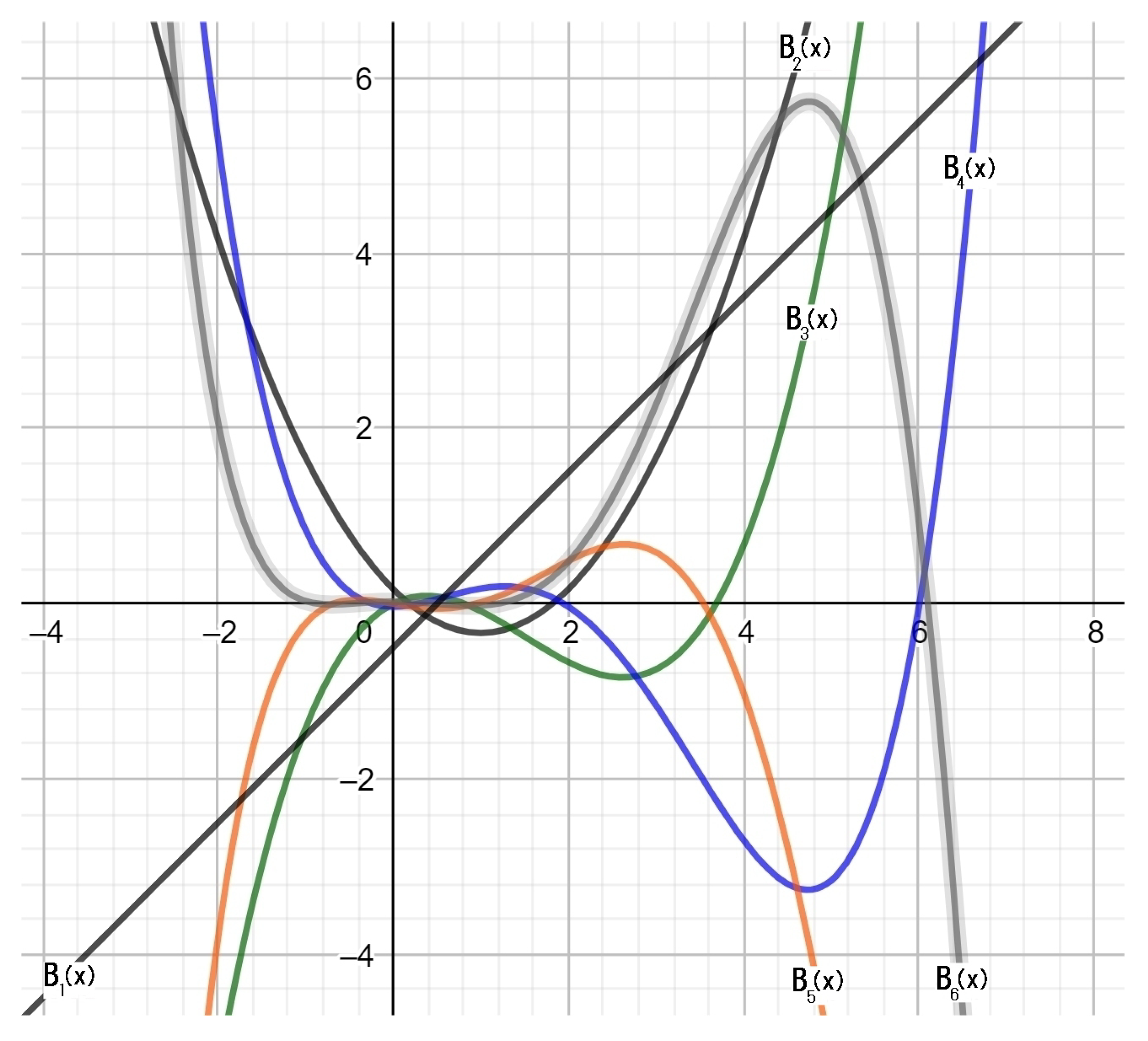
The first few L-Bernoulli polynomials are as follows (Figure 1).

$$\begin{array}{c}\begin{array}{c}{}_L{B}_0\left(x\right)=1\hfill \\ {}_L{B}_1\left(x\right)=x-\frac{1}{2}\hfill \\ {}_L{B}_2\left(x\right)=\frac{x^2}{2}-x+\frac{1}{6}\hfill \\ {}_L{B}_3\left(x\right)=\frac{x^3}{6}-\frac{3}{4}{x}^2+\frac{1}{2}x\hfill \\ {}_L{B}_4\left(x\right)=\frac{x^4}{24}-\frac{1}{3}{x}^3+\frac{1}{2}{x}^2-\frac{1}{30}\hfill \\ {}_L{B}_5\left(x\right)=\frac{x^5}{120}-\frac{5}{48}{x}^4+\frac{5}{18}{x}^3-\frac{1}{6}x\hfill \\ {}_L{B}_6\left(x\right)=\frac{x^6}{720}-\frac{1}{40}{x}^5+\frac{5}{48}{x}^4-\frac{1}{4}{x}^2+\frac{1}{42}\hfill \\ {}_L{B}_7\left(x\right)=\frac{x^7}{5040}-\frac{7}{1440}{x}^6+\frac{7}{240}{x}^5-\frac{7}{36}{x}^3+\frac{1}{6}x\hfill \\ {}_L{B}_8\left(x\right)=\frac{x^8}{40320}-\frac{1}{1260}{x}^7+\frac{7}{1080}{x}^6-\frac{7}{72}{x}^4+\frac{1}{3}{x}^2-\frac{1}{30}\hfill \\ {}_L{B}_9\left(x\right)=\frac{x^9}{362880}-\frac{1}{8960}{x}^8+\frac{1}{840}{x}^7-\frac{7}{200}{x}^5+\frac{1}{3}{x}^3-\frac{3}{10}x\hfill \end{array}\end{array}$$

Note that, as the operator $Dx{D}^0=Id$, the identity operator, we have $\forall n\in \mathbf{N}$—${}_L{B}_n\left(0\right)={}_L{B}_n=B_n$, that is.

The L-Bernoulli numbers are the same as the ordinary Bernoulli numbers.

Although this article is mainly focused on Bernoulli-type polynomials, it should be noted that many extensions can be made, for example, by considering the Genocchi polynomials or the polynomials of Apostol-Bernoulli polynomials of order $\alpha$, studied in [36], which are defined by means of the exponential generating function

$$\begin{array}{c}\hfill {\left(\frac{t{e}^{xt}}{\lambda e^t-1}\right)}^{\alpha }{e}^{xt}=\sum _{n=0}^{\infty }{\mathcal{B}}_n^{\alpha }(x;\lambda )\frac{t^n}{n!},\left(\right|t+log\lambda |<2\pi ;1^{\alpha }:=1),\end{array}$$

where, denoting by $B_n^{\alpha }\left(x\right)$ the Bernoulli-Apostol polynomials [37], it results in

$$\begin{array}{c}\hfill B_n^{\alpha }\left(x\right)={\mathcal{B}}_n^{\alpha }(x;1),\mathrm{and}{\mathcal{B}}_n^{\alpha }\left(\lambda \right):={\mathcal{B}}_n^{\alpha }(0;\lambda ),\end{array}$$

and ${\mathcal{B}}_n^{\alpha }\left(\lambda \right)$ are the Apostol-Bernoulli numbers of order $\alpha$, generalizing the classical ones.

The Laguerre-type Apostol-Bernoulli polynomials of order $\alpha$ are obtained by means of the exponential generating function

$$\begin{array}{c}\hfill {\left(\frac{t{e}_1\left(xt\right)}{\lambda e_1\left(t\right)-1}\right)}^{\alpha }{e}^{xt}=\sum _{n=0}^{\infty }{}_L{\mathcal{B}}_n^{\alpha }(x;\lambda )\frac{t^n}{n!},\left(\right|t+log\lambda |<2\pi ;1^{\alpha }:=1),\end{array}$$

Similar definitions for the Apostol-Euler numbers of order $\alpha$ can be found in the same article [36].

3.3. Laguerre-Type Euler Polynomials

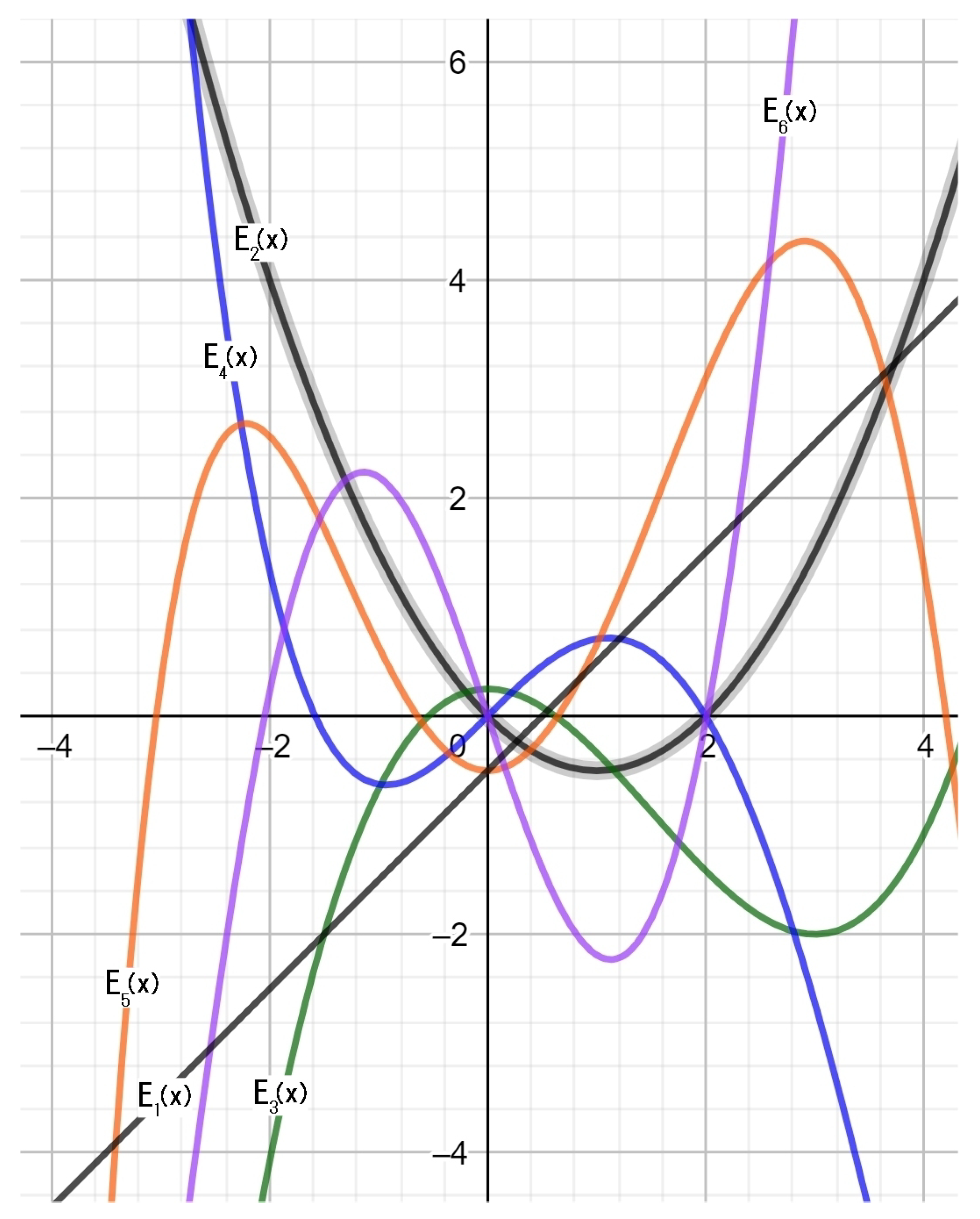
The first few L-Euler polynomials are as follows (Figure 2).

$$\begin{array}{c}\hfill \begin{array}{c}{}_L{E}_0\left(x\right)=1\hfill \\ {}_L{E}_1\left(x\right)=x-\frac{1}{2}\hfill \\ {}_L{E}_2\left(x\right)=\frac{x^2}{2}-x\hfill \\ {}_L{E}_3\left(x\right)=\frac{x^3}{6}-\frac{3}{4}{x}^2+\frac{1}{4}\hfill \\ {}_L{E}_4\left(x\right)=\frac{x^4}{24}-\frac{1}{3}{x}^3+x\hfill \\ {}_L{E}_5\left(x\right)=\frac{x^5}{120}-\frac{5}{48}{x}^4+\frac{5}{4}{x}^2-\frac{1}{2}\hfill \\ {}_L{E}_6\left(x\right)=\frac{x^6}{720}-\frac{1}{40}{x}^5+\frac{5}{6}{x}^3-3x\hfill \\ {}_L{E}_7\left(x\right)=\frac{x^7}{5040}-\frac{7}{1440}{x}^6+\frac{35}{96}{x}^4-\frac{21}{4}{x}^2+\frac{17}{8}\hfill \\ {}_L{E}_8\left(x\right)=\frac{x^8}{40320}-\frac{1}{1260}{x}^7+\frac{7}{60}{x}^5-\frac{14}{3}{x}^3+17x\hfill \\ {}_L{E}_9\left(x\right)=\frac{x^9}{362880}-\frac{1}{8960}{x}^8+\frac{7}{240}{x}^6-\frac{21}{8}{x}^4+\frac{135}{4}{x}^2-\frac{31}{2}\hfill \end{array}\end{array}$$

In addition, in this case we have $\forall n\in \mathbf{N}$—${}_L{E}_n\left(0\right)={}_L{E}_n=E_n$, that is.

The L-Euler numbers are the same as the ordinary Euler numbers.

3.4. Main Properties

Being a particular case of the L-Appell polynomials, the L-Bernoulli and L-Euler polynomials also satisfy the equations

$$\begin{array}{c}{D}_L\left[{{}_{L}B}_n\left(x\right)\right]=n\left[{{}_{L}B}_{n-1}\left(x\right)\right],\hfill \\ D_L\left[{{}_{L}E}_n\left(x\right)\right]=n\left[{{}_{L}E}_{n-1}\left(x\right)\right].\hfill \end{array}$$

(12)

Equations (12) are iterated as

$$\begin{array}{c}\begin{array}{c}{\left(D_L\right)}^m\left[{{}_{L}B}_n\left(x\right)\right]=D^m{x}^m{D}^m\left[{{}_{L}B}_n\left(x\right)\right]=\frac{n!}{(n-m)!}\left[{{}_{L}B}_{n-m}\left(x\right)\right],\hfill \\ {\left(D_L\right)}^m\left[{{}_{L}E}_n\left(x\right)\right]=D^m{x}^m{D}^m\left[{{}_{L}E}_n\left(x\right)\right]=\frac{n!}{(n-m)!}\left[{{}_{L}E}_{n-m}\left(x\right)\right],\hfill \end{array}\end{array}$$

Theorem 2.

The following properties hold:

• By introducing the 2nd kind L-Stirling numbers ${}_{L}S(n,k)$ defined as

  $$\begin{array}{c}\hfill \begin{array}{c}{}_{L}S(n,k)=S(n,k)n!,(n\in \mathbf{N},k=0,1,\dots ,n-1),\hfill \end{array}\end{array}$$

  (13)
  we find

  $$\begin{array}{c}\hfill \begin{array}{c}{\left(x\right)}_n=x(x-1)\cdots (x-n+1)={\displaystyle \sum _{k=0}^n}{}_{L}S(n,k\frac{x^n}{n!}).\hfill \end{array}\end{array}$$

  (14)
• This results in

  $$\begin{array}{c}\hfill \begin{array}{c}\frac{1}{n+1}{\displaystyle \sum _{k=0}^n}\left(\genfrac{}{}{0pt}{}{n+1}{k}\right){}_L{B}_k\left(x\right)=\frac{x^n}{n!},\hfill \end{array}\end{array}$$

  (15)
• The integral relations hold:

  $$\begin{array}{c}\hfill \begin{array}{c}{\int }_a^y\frac{1}{x}{\int }_0^x{{}_{L}B}_n\left(t\right)dtdy=\frac{{}_L{B}_{n+1}\left(y\right)-{}_L{B}_{n+1}\left(a\right)}{n+1},\hfill \\ \phantom{1pt32pt}{\int }_a^y\frac{1}{x}{\int }_0^x{{}_{L}E}_n\left(t\right)dtdy=\frac{{}_L{E}_{n+1}\left(y\right)-{}_L{E}_{n+1}\left(a\right)}{n+1}.\hfill \end{array}\end{array}$$

  (16)

Proof. 

The three preceding results follow from a straightforward application of the isomorphism $T_x$ to both sides of the corresponding equations valid for the ordinary Bernoulli polynomials. Formulas (16) are obtained by inverting the Laguerre derivative operator. □

A general result on differential equations satisfied by Appell polynomials is reported in [38]. This result could be applied even in the Laguerre-type case, substituting the ordinary with the Laguerre derivative, but we do not go further in this direction because of the Ismail’s remark states that it is not clear to introduce differential equations of this kind which do not have a finite order.

4. Hypergeometric L-Bernoulli Polynomials

Putting

$$\begin{array}{c}\hfill {}_L{T}_r\left(x\right)=\sum _{k=0}^r\frac{x^k}{{(k!)}^2}\end{array}$$

(17)

and

$$\begin{array}{c}\hfill {{}_{1}F}_2(1;r+1,r+1;x)=\sum _{h=0}^{\infty }\frac{x^h}{{\left[{(r+1)}_h\right]}^2}=\sum _{h=0}^{\infty }\frac{{\left(1\right)}_h}{{\left[{(r+1)}_h\right]}^2}\frac{x^h}{h!},\end{array}$$

(18)

since

$$\begin{array}{c}\hfill e_1\left(x\right)-{{}_{L}T}_r\left(x\right)=\sum _{n=r}^{\infty }\frac{x^n}{{(n!)}^2}=x^r\sum _{n=0}^{\infty }\frac{1}{{[(n+r)!]}^2}{x}^n,\end{array}$$

(19)

and

$$\begin{array}{c}\hfill \frac{\frac{x^r}{{(r!)}^2}{e}_1\left(tx\right)}{e_1\left(x\right)-{{}_{L}T}_r\left(x\right)}=\frac{e_1\left(tx\right)}{{(r!)}^2{\displaystyle \sum _{n=0}^{\infty }}\frac{x^n}{{[(n+r)!]}^2}},\end{array}$$

(20)

We have the exponential generating function of the hypergeometric Bernoulli polynomials ${}_L{B}_n^{[r-1,1]}\left(t\right)$, where the classical gamma function is used:

$$\begin{array}{c}\hfill \frac{e_1\left(tx\right)}{{\left[\mathrm{\Gamma }(r+1)\right]}^2{\displaystyle \sum _{n=0}^{\infty }}\frac{1}{{\left[\mathrm{\Gamma }(n+r+1)\right]}^2}{x}^n}=\sum _{n=0}^{\infty }{{}_{L}B}_n^{[r-1,1]}\left(t\right)\frac{x^n}{n!}.\end{array}$$

(21)

Remark 4.

Note that, since the isomorphism ${\mathcal{T}}_x$ does not preserve multiplication, the ${{}_L{B}^{[r-1,1]}}_n$ polynomials, as the more general ones presented in subsequent Sections, are independent of those presented in [24].

4.1. Computing the Hypergeometric L-Bernoulli Numbers by Recursion

In (21), making $t=0$ gives the exponential generating function [1] of the generalized hypergeometric L-Bernoulli numbers ${}_L{B}_n^{[r-1,1]}:={{}_{L}B}_n^{[r-1,1]}\left(0\right)$:

$$\begin{array}{c}\hfill \sum _{n=0}^{\infty }{{}_{L}B}_n^{[r-1,1]}\frac{x^n}{n!}=\frac{1}{{\left[\mathrm{\Gamma }(r+1)\right]}^2{\displaystyle \sum _{n=0}^{\infty }}\frac{n!}{{\left[\mathrm{\Gamma }(n+r+1)\right]}^2}\frac{x^n}{n!}},\end{array}$$

(22)

which is valid even for non integer (in particular for fractional) values of the parameter r.

From Equation (22), we find

$$\begin{array}{c}\hfill \sum _{n=0}^{\infty }\sum _{h=0}^n\left(\genfrac{}{}{0pt}{}{n}{h}\right){{}_{L}B}_{n-h}^{[r-1,1]}\frac{h!{\left[\mathrm{\Gamma }(r+1)\right]}^2}{{\left[\mathrm{\Gamma }(h+r+1)\right]}^2}\frac{x^n}{n!}=1,\end{array}$$

and therefore

$$\begin{array}{c}\hfill {}_L{B}_0^{[r-1,1]}=1,\end{array}$$

and for $n=1,2,3,\dots$, we find the ${}_L{B}_n^{[r-1,1]}$ numbers by solving recursively the triangular system:

$$\begin{array}{c}\hfill \sum _{h=0}^n\left(\genfrac{}{}{0pt}{}{n}{h}\right){{}_{L}B}_{n-h}^{[r-1,1]}\frac{h!{\left[\mathrm{\Gamma }(r+1)\right]}^2}{{\left[\mathrm{\Gamma }(h+r+1)\right]}^2}=0.\end{array}$$

4.2. Hypergeometric L-Bernoulli Polynomials of Order 2

The results of the preceding section can be generalized to the hypergeometric L-Bernoulli polynomials of order 2, which are defined by the generating function

$$\begin{array}{c}\hfill \frac{{\left[\frac{x^r}{{(r!)}^2}\right]}^2{e}_1\left(tx\right)}{{[e_1\left(x\right)-{{}_{L}T}_r\left(x\right)]}^2}=\frac{e_1\left(tx\right)}{{{[}_1{F}_2(1;r+1,r+1;x)]}^2}=\sum _{n=0}^{\infty }{{}_{L}B}_n^{[r-1,2]}\left(t\right)\frac{x^n}{n!}.\end{array}$$

(23)

We find

$$\begin{array}{c}\hfill \begin{array}{c}{{[}_1{{}_{L}F}_1]}^2={\displaystyle \sum _{n=0}^{\infty }}{\displaystyle \sum _{h=0}^n}\left(\genfrac{}{}{0pt}{}{n}{h}\right)\frac{{\left(1\right)}_h{\left(1\right)}_{n-h}}{{\left[{(r+1)}_h\right]}^2{\left[{(r+1)}_{n-h}\right]}^2}\frac{x^n}{n!}\\ ={\displaystyle \sum _{n=0}^{\infty }}{\displaystyle \sum _{h=0}^n}\frac{x^n}{{\left[{(r+1)}_h\right]}^2{\left[{(r+1)}_{n-h}\right]}^2},\end{array}\end{array}$$

(24)

so that

$$\begin{array}{c}\hfill \frac{e_1\left(tx\right)}{{\displaystyle \sum _{n=0}^{\infty }}{\displaystyle \sum _{h=0}^n}\frac{x^n}{{\left[{(r+1)}_h\right]}^2{\left[{(r+1)}_{n-h}\right]}^2}}=\sum _{n=0}^{\infty }{{}_{L}B}_n^{[r-1,2]}\left(t\right)\frac{x^n}{n!},\end{array}$$

(25)

and introducing the hypergeometric L-Bernoulli numbers ${{}_{L}B}_n^{[r-1,2]}:={{}_{L}B}_n^{[r-1,2]}\left(0\right)$, we find the generating function

$$\begin{array}{c}\hfill \frac{1}{{\displaystyle \sum _{n=0}^{\infty }}{\displaystyle \sum _{h=0}^n}\frac{x^n}{{\left[{(r+1)}_h\right]}^2{\left[{(r+1)}_{n-h}\right]}^2}}=\sum _{n=0}^{\infty }{{}_{L}B}_n^{[r-1,2]}\frac{x^n}{n!},\end{array}$$

(26)

which gives the generating function of the hypergeometric L-Bernoulli numbers ${{}_{L}B}_n^{[r-1,2]}$

$$\begin{array}{c}\hfill \frac{1}{{\displaystyle \sum _{n=0}^{\infty }}{\displaystyle \sum _{h=0}^n}\frac{{\left[\mathrm{\Gamma }(r+1)\right]}^4}{{\left[\mathrm{\Gamma }(r+h+1)\right]}^2{\left[\mathrm{\Gamma }(r+n-h+1)\right]}^2}{x}^n}=\sum _{n=0}^{\infty }{{}_{L}B}_n^{[r-1,2]}\frac{x^n}{n!}.\end{array}$$

(27)

5. Conclusions

We have introduced the Laguerre-type versions of some special polynomials as the Appell, Bernoulli and Euler versions. The results followed from the application of the differential isomorphism ${\mathcal{T}}_x$ introduced in [26]. Generalization can be done by exploiting the iterated isomorhism ${\mathcal{T}}_x^s={\mathcal{T}}_x{\left[{\mathcal{T}}^{s-1}\right]}_x$, recalled in Section 2. The considered isomorphism can be iterated as many times as we wish, and the corresponding derivative operators are reported in Equation (9). Then, by using the same technique, it is possible to define higher order L-Appell type polynomials

$${}_{L^2}{a}_n\left(x\right),{}_{L^3}{a}_n\left(x\right),\dots ,{}_{L^s}{a}_n\left(x\right),\dots$$

and in particular, those of Bernoulli or Euler type.

Furthermore, we have considered the hypergeometric-type L-Bernoulli polynomials of order 1 and 2, starting from the exponential generating functions considered in [24].

The higher-order, hypergeometric-type L-Bernoulli polynomials of order k, with $k=3,4,\dots$ and $s\ge 2$, could be defined through the generating function

$$\begin{array}{c}\hfill \frac{{\left[\frac{x^r}{{(r!)}^{s+1}}\right]}^k{e}_s\left(tx\right)}{{[e_s\left(x\right)-{{}_{L^s}T}_r\left(x\right)]}^k}=\frac{e_s\left(tx\right)}{{{[}_1{F}_s(1;r+1,r+1;\dots ;r+1;x)]}^k}=\sum _{n=0}^{\infty }{{}_{L^s}B}_n^{[r-1,k]}\left(t\right)\frac{x^n}{n!},\end{array}$$

(28)

and the corresponding numbers ${{}_{L^s}B}_n^{[r-1,k]}$ by

$$\begin{array}{c}\hfill \frac{{\left[\frac{x^r}{{(r!)}^{s+1}}\right]}^k}{{[e_s\left(x\right)-{{}_{L^s}T}_r\left(x\right)]}^k}=\frac{1}{{{[}_1{F}_s(1;r+1,r+1;\dots ;r+1;x)]}^k}=\sum _{n=0}^{\infty }{{}_{L^s}B}_n^{[r-1,k]}\frac{x^n}{n!}.\end{array}$$

(29)

However, as mentioned earlier, the construction of these mathematical items does not present difficulties, since the method is essentially the same.

References

- Srivastava, H.M.; Manocha, H.L. A Treatise on Generating Functions; Halsted Press (Ellis Horwood Limited): Chichester, UK; John Wiley and Sons: New York, NY, USA; Chichester, UK; Brisbane, Australia; Toronto, Japan, 1984. [Google Scholar]
- Srivastava, H.M.; Çetinkaya, A.; Kımaz, O. A certain generalized Pochhammer symbol and its applications to hypergeometric functions. Appl. Math. Comput. 2014, 226, 484–491. [Google Scholar] [CrossRef]
- Srivastava, H.M.; Kizilateş, C. A parametric kind of the Fubini-type polynomials. Rev. Real Acad. Cienc. Exactas Físicas Nat. Ser. A Mat. 2019, 113, 3253–3267. [Google Scholar] [CrossRef]
- Srivastava, H.M.; Ricci, P.E.; Natalini, P. A family of complex Appell polynomial sets. Rev. Real Acad. Cienc. Exactas Físicas Nat. Ser. A Mat. 2019, 113, 2359–2371. [Google Scholar] [CrossRef]
- Srivastava, H.M.; Riyasat, M.; Khan, S.; Araci, S.; Acikgoz, M. A new approach to Legendre-truncated-exponential-based Sheffer sequences via Riordan arrays. Appl. Math. Comput. 2020, 369, 124683. [Google Scholar] [CrossRef]
- Srivastava, R.; Cho, N.E. Generating functions for a certain class of incomplete hypergeometric polynomials. Appl. Math. Comput. 2012, 219, 3219–3225. [Google Scholar] [CrossRef]
- Srivastava, R. Some properties of a family of incomplete hypergeometric functions. Russ. J. Math. Phys. 2013, 20, 121–128. [Google Scholar] [CrossRef]
- Srivastava, R.; Cho, N.E. Some extended Pochhammer symbols and their applications involving generalized hypergeometric polynomials. Appl. Math. Comput. 2014, 234, 277–285. [Google Scholar] [CrossRef]
- Srivastava, R. Some classes of generating functions associated with a certain family of extended and generalized hypergeometric functions. Appl. Math. Comput. 2014, 243, 132–137. [Google Scholar] [CrossRef]
- Dilcher, K. A Bibliography of Bernoulli Numbers. Available online: www.mathstat.dal.ca/dilcher/bernoulli.html (accessed on 1 May 2022).
- Smith, D.E. A Source Book in Mathematics; McGraw-Hill: New York, NY, USA, 1929. [Google Scholar]
- Bretti, G.; Natalini, P.; Ricci, P.E. Generalizations of the Bernoulli and Appel polynomials. Abstr. Appl. Anal. 2004, 7, 613–623. [Google Scholar] [CrossRef] [Green Version]
- Howard, F.T. Numbers Generated by the Reciprocal of ex-x-1. Math. Comput. 1977, 31, 581–598. [Google Scholar]
- Srivastava, H.M.; Todorov, P.G. An Explicit Formula for the Generalized Bernoulli Polynomials. J. Math. Anal. Appl. 1988, 130, 509–513. [Google Scholar] [CrossRef] [Green Version]
- Natalini, P.; Bernardini, A. A generalization of the Bernoulli polynomials. J. Appl. Math. 2003, 3, 155–163. [Google Scholar] [CrossRef] [Green Version]
- Hassen, A.; Nguyen, H.D. Hypergeometric Bernoulli polynomials and Appell sequences. Int. J. Number Theory 2008, 4, 767–774. [Google Scholar] [CrossRef] [Green Version]
- Kurt, B. A Further Generalization of the Bernoulli Polynomials and on the 2D-Bernoulli Polynomials (x, y). Appl. Math. Sci. 2010, 4, 2315–2322. [Google Scholar]
- Booth, R.; Hassen, A. Hypergeometric Bernoulli polynomials. J. Algebra Number Theory 2011, 2, 1–7. [Google Scholar]
- Kurt, B. Some Relationships between the Generalized Apostol-Bernoulli and Apostol-Euler Polynomials. Turk. J. Anal. Number Theory 2013, 1, 54–58. [Google Scholar] [CrossRef]
- Hu, S.; Kim, M.-S. On hypergeometric Bernoulli numbers and polynomials. Acta Math. Hungar. 2018, 154, 134–146. [Google Scholar] [CrossRef] [Green Version]
- Geleta, H.L.; Hassen, A. Fractional hypergeometric zeta functions. Ramanujan J. 2016, 41, 421–436. [Google Scholar] [CrossRef]
- Miloud, M.; Tiachachat, M. The values of the high order Bernoulli polynomials at integers and the r-Stirling numbers. arXiv 2014, arXiv:1401.5958. [Google Scholar]
- Miloud, M.; Tiachachat, M. A new class of the r-Stirling numbers and the generalized Bernoulli polynomials. Integers 2020, 20, 1–8. [Google Scholar]
- Ricci, P.E.; Natalini, P. Hypergeometric Bernoulli polynomials and r-associated Stirling numbers of the second kind. Integers 2022, in press. [Google Scholar]
- Ricci, P.E. Laguerre-Type Exponentials, Laguerre Derivatives and Applications. A Survey. Mathematics 2020, 8, 2054. [Google Scholar] [CrossRef]
- Ricci, P.E.; Tavkhelidze, I. An introduction to operational techniques and special polynomials. J. Math. Sci. 2009, 157, 161–189. [Google Scholar] [CrossRef]
- Dattoli, G. Hermite-Bessel and Laguerre-Bessel functions: A by-product ot the monomiality principle. In Advanced Special Functions and Applications, Proceedings of the Melfi School on Advanced Topics in Mathematics and Physics; Melfi, 9–12 May 1999; Cocolicchio, D., Dattoli, G., Srivastava, H.M., Eds.; Aracne Editrice: Rome, Italy, 2000; pp. 147–164. [Google Scholar]
- Dattoli, G.; Ricci, P.E. Laguerre-type exponentials, and the relevant L-circular and L-hyperbolic functions. Georgian Math. J. 2003, 10, 481–494. [Google Scholar] [CrossRef]
- Ditkin, V.A.; Prudnikov, A.P. Integral Transforms and Operational Calculus; Pergamon Press: Oxford, UK, 1965. [Google Scholar]
- Dimovski, I. Operational calculus for a class of differential operators. CR Acad. Bulg. Sci. 1966, 19, 1111–1114. [Google Scholar]
- Kilbas, A.A.; Srivastava, H.M.; Trujillo, J.J. Theory and Applications of Fractional Differential Equations, North-Holland Mathematical Studies; Elsevier (North-Holland) Science Publishers: Amsterdam, The Netherlands; London UK; New York, NY, USA, 2006; Volume 204. [Google Scholar]
- Penson, K.A.; Blasiak, P.; Horzela, A.; Solomon, A.I.; Duchamp, G.H.E. Laguerre-type derivatives: Dobiński relations and combinatorial identities. J. Math. Phys. 2009, 50, 3512. [Google Scholar] [CrossRef] [Green Version]
- Bretti, G.; Cesarano, C.; Ricci, P.E. Laguerre-type exponentials and generalized Appell polynomials. Comput. Math. Appl. 2004, 48, 833–839. [Google Scholar] [CrossRef] [Green Version]
- Viskov, O.V. A commutative-like noncommutation identity. Acta Sci. Math. 1994, 59, 585–590. [Google Scholar]
- Boas, R.P.; Buck, R.C. Polynomial Expansions of Analytic Functions; Springer: Berlin/Heidelberg, Germany, 1958. [Google Scholar]
- Luo, Q.-M.; Srivastava, H.M. Some generalizations of the Apostol-Bernoulli and Apostol–Euler polynomials. J. Math. Anal. Appl. 2005, 308, 290–302. [Google Scholar] [CrossRef]
- Apostol, T.M. Introduction to Analytic Number Theory; Springer: New York, NY, USA, 1976. [Google Scholar]
- Ismail, M.E.H. Remarks on “Differential equation of Appell polynomials”. J. Comp. Appl. Math. 2003, 154, 243–245. [Google Scholar] [CrossRef] [Green Version]
Figure 1.
Graphs of polynomials for .
Figure 2.
Publisher’s Note: MDPI stays neutral with regard to jurisdictional claims in published maps and institutional affiliations. |
© 2022 by the authors. Licensee MDPI, Basel, Switzerland. This article is an open access article distributed under the terms and conditions of the Creative Commons Attribution (CC BY) license (https://creativecommons.org/licenses/by/4.0/).
Share and Cite
MDPI and ACS Style
Ricci, P.E.; Srivastava, R. A Note on the Laguerre-Type Appell and Hypergeometric Polynomials. Mathematics 2022, 10, 1951. https://0-doi-org.brum.beds.ac.uk/10.3390/math10111951
AMA Style
Ricci PE, Srivastava R. A Note on the Laguerre-Type Appell and Hypergeometric Polynomials. Mathematics. 2022; 10(11):1951. https://0-doi-org.brum.beds.ac.uk/10.3390/math10111951
Chicago/Turabian StyleRicci, Paolo Emilio, and Rekha Srivastava. 2022. "A Note on the Laguerre-Type Appell and Hypergeometric Polynomials" Mathematics 10, no. 11: 1951. https://0-doi-org.brum.beds.ac.uk/10.3390/math10111951
Note that from the first issue of 2016, this journal uses article numbers instead of page numbers. See further details here.