Calculating Complete Lists of Belyi Pairs

Abstract

Belyi pairs constitute an important element of the program developed by Alexander Grothendieck in 1972–1984. This program related seemingly distant domains of mathematics; in the case of Belyi pairs, such domains are two-dimensional combinatorial topology and one-dimensional arithmetic geometry. The paper contains an account of some computer-assisted calculations of Belyi pairs with fixed discrete invariants. We present three complete lists of polynomial-like Belyi pairs: (1) of genus 2 and (minimal possible) degree 5; (2) clean ones of genus 1 and degree 8; and (3) clean ones of genus 2 and degree 8. The explanation of some phenomena we encounter in these calculations will hopefully stimulate further development of the dessins d’enfants theory.

1. Introduction

By definition, a Belyi pair is a pair $(\mathbf{X},\beta )$, where $\mathbf{X}$ is a complete smooth irreducible curve over an algebraically closed field $\mathbb{k}$ and $\beta$ is a rational non-constant function on $\mathbf{X}$ with only three critical values. This short definition covers some enigmatic relations between several domains of mathematics. In the present paper, we mention just one of such relations that motivate the thorough investigation of Belyi pairs.

We identify the rational functions $f\in \mathbb{k}\left(\mathbf{X}\right)$ and the branched covers of the projective line $f:\mathbf{X}\to {\mathbf{P}}_1\left(\mathbb{k}\right)$. For a non-constant $f\in \mathbb{k}\left(\mathbf{X}\right)\backslash \mathbb{k}$, denote the set of its critical values by

$$\mathrm{CritVal}\left(f\right):=\{c\in {\mathbf{P}}_1\left(\mathbb{k}\right)\mid \#f^{-1\circ }\left(c\right)<deg\left(f\right)\}.$$

According to these notations, a Belyi pair is a pair $(\mathbf{X},\beta )$ with such $\beta \in \mathbb{k}\left(\mathbf{X}\right)\backslash \mathbb{k}$ that

$$\#\mathrm{CritVal}\left(\beta \right)\le 3.$$

The cases with $\#\mathrm{CritVal}\left(\beta \right)<3$ are of little interest:

• $\#\mathrm{CritVal}\left(\beta \right)=0$ implies $\mathbf{X}={\mathbf{P}}_1\left(\mathbb{k}\right)$ and $\beta \left(z\right)=(az+b)/(cz+d)$;
• $\#\mathrm{CritVal}\left(\beta \right)=1$ is impossible;
• $\#\mathrm{CritVal}\left(\beta \right)=2$ implies $\mathbf{X}={\mathbf{P}}_1\left(\mathbb{k}\right)$ and $\beta$ is equivalent to $z\to z^n$ with $n\in \mathbb{N}$, $n_{\ge }2$.

Hence, we will consider only the case

$$\#\mathrm{CritVal}\left(\beta \right)=3.$$

Moreover, by post-composing $\beta$ with an appropriate fractional-linear transformation, we can assume that

$$\mathrm{CritVal}\left(\beta \right)=\{0,1,\infty \}$$

and in most cases, we stick to this assumption.

A Belyi pair $(\mathbf{X},\beta )$ is called clean if all the ramifications of $\beta$ over 1 are 2-fold; in other words, for $P\in \mathbf{X}$

$$\left[\beta \right(P)=1]⟹[\beta -1\in 〈{\mathfrak{m}}_P^2〉\backslash 〈{\mathfrak{m}}_P^3〉],$$

where ${\mathfrak{m}}_P◃{\mathcal{O}}_P$ is the maximal ideal in the local ring of a point P, and for a set $S\subset {\mathcal{O}}_P$, we denote by $\langle S\rangle$ the ideal generated by S.

From now on, assume

$$\mathrm{char}\left(\mathbb{k}\right)\ne 2.$$

Then, the assumption of cleanness is not really restrictive since, for any Belyi pair, $(\mathbf{X},\beta )$ the pair $\left(\mathbf{X},4\beta (1-\beta )\right)$ is clean.

Over the ground field $\mathbb{k}=\mathbb{C}$, the relation of Belyi pairs with combinatorial topology is rather direct. If $(\mathbf{X},\beta )$ is a clean Belyi pair over $\mathbb{C}$, then the pre-image of the segment ${\mathbf{X}}_1:={\beta }^{-1\circ }[0,1]$ is such a graph

$${\mathbf{X}}_1\subset \mathbf{X}$$

that

$$thecomplement\mathbf{X}\backslash {\mathbf{X}}_{1}ishomeomorphictoadisjointunionof2cells.$$

(1)

The embeddings ${\mathbf{X}}_1\hookrightarrow \mathbf{X}$ of graphs into compact oriented surfaces enjoying this property were studied for some time—see, e.g., [1]. From the combinatorial point of view, it looks like a natural partner of the classical theory of graph enumeration (see [2]). However, the theory of graph embeddings satisfying (1) turned out to be much more related to other domains of mathematics and physics. An example of relations with gauge theories can be found in [3]; relations with computer science and neural networks are discussed in [4].

From now on, we return to algebraic geometry.

Alexander Grothendieck, one of the central figures of algebraic geometry in 20th century, became interested in the embeddings satisfying (1) in rather peculiar circumstances. In the beginning of the 1970s, he abandoned the mathematical community for certain non-mathematical reasons (see mathematicians’ explanations in [5]) and returned to his mother university in Montpellier. There, he had to supervise the research of students with a very modest background, so Grothendieck’s native domains turned out to be inappropriate. Having to choose some elementary one, he started to study (assisted a bit by his students) the graphs on surfaces with the property (1). He called them dessins d’enfants due to their apparent simplicity, and in some time, this term became more popular than the previous ones—maps, orgraphs, etc.

The Montpellier period of Grothendieck’s active mathematical life is covered approximately by the years 1972–1984. During the first half of this period, he worked as a combinatorial topologist and rediscovered a beautiful group-theoretical method of describing dessins d’enfants. However, the most important event happened in the middle of this period: in 1978, he became aware (thanks to their former student Pierre Deligne with whom he still kept in contact) of the result of the Soviet mathematician Gennady Belyi [6]. According to Belyi’s theorem, the (appropriately defined) category of dessins d’enfants is equivalent not only to the category of Belyi pairs over $\mathbb{C}$ (which is more or less clear from the above explanations) but to such a category over the field $\overline{\mathbb{Q}}$ of algebraic numbers!

Grothendieck was emotionally struck with this result and saw it as a fantastic one. From a personal point of view, it meant that his attempt to abandon algebraic geometry in favor of more elementary objects failed: the two turned out to be firmly related. From the general mathematical perspective, putting together the mentioned results provide the action of the absolute Galois group $\mathrm{Aut}\left(\overline{\mathbb{Q}}\right)$ on the isotopy classes of dessins d’enfants! It was realized soon (see [7]) that this action is faithful.

Thus, the theory of dessins d’enfants provides the unique opportunity of the visualization of the absolute Galois group. Of course, this is just one of the many consequences of the above category equivalence, but it is one of the main motivations of the calculations presented below.

In more general terms, we have two very different categories of objects: ${\mathcal{C}}_1$ and ${\mathcal{C}}_2$ (in our case, dessins d’enfants and Belyi pairs over $\overline{\mathbb{Q}}$). The categories are essentially small (the term suggested by P. Deligne instead of the existence of a small subcategory containing object of all the classes of isomorphism), i.e., the classes of their isomorphic objects constitute sets. Denote these sets $|{\mathcal{C}}_1|$ and $|{\mathcal{C}}_2|$. Each object of both categories is defined by a finite amount of information, and there is a theory establishing the one-to-one correspondence

$$|{\mathcal{C}}_1|\stackrel{\cong }{⟷}\left|{\mathcal{C}}_2\right|$$

(2)

The true nature of this correspondence for the time being is understood poorly; otherwise, its existence would not be so surprising. In the hope of its better understanding, the authors participate for several decades in the calculation of particular cases. (It is a rather active international activity, see, e.g., [8].) In the present paper, we demonstrate some results obtained on the PC’s using MAPLE and avoiding any advanced techniques of calculation. Our strategy is to analyze (2) as detailed as possible within the objects of bounded complexity (the number of edges and the genus of the surface on the one hand and the degree of Belyi map and the genus on the other).

The dissemination of the dessins d’enfants theory was initiated by the famous informal text [9]. The rigorous basic definitions of this theory, and the main theorems together with the first examples were published in [10]; the monographic expositions can be found in [11,12]. The papers [13,14] contain more recent overviews, including some computer calculations.

The previously known calculations of Belyi pairs of positive genus are mostly related to the special (highly symmetrical) curves; they were investigated actively since 18th–19th century by Bring, Hurwitz, Klein, Wiman, etc. For the general dessins of positive genus, the known results are somewhat fragmentary. The ongoing project of compiling the database of Belyi pairs (see the recent report [8]) covers the complete lists up to degree 6 and some fragmentary results up to degree 9 and genus $\le 3$. The complete list of the clean Belyi pairs with $\le 4$ edges (and hence degree $\le 8$), containing 134 cases, was published in the catalog [15] without calculations. In the present paper, the details of the calculations of all four cases of genus 2 are given, two of them rather hard and requiring computer calculations. These results are presumably new.

The authors are indebted to the participants of the Moscow State University seminar “Graphs on surfaces and curves over number fields”, A. D. Mednykh and A. K. Zvonkin, for their interest. The most difficult results of this paper could not be obtained without the contribution of S. Yu. Orevkov, who performed some computer calculations several years ago.

2. Belyi Pairs of Genera 0 and 1

2.1. On Plane Trees

In the genus-0 case, the most complete results are known when there is only one cell in the above condition (1), i.e., when the complement ${\mathbf{S}}^2\backslash {\mathbf{X}}_1$ in the 2-sphere is homeomorphic to the disk. It happens if ${\mathbf{X}}_1$ is a tree; the corresponding Belyi functions are called Shabat polynomials. The general self-contained introduction to the theory can be found in [16].

The first complete list of plane trees and their Shabat polynomials was presented in [17]; it covered the trees with ≤ eight edges. The trees with nine edges were covered in [18] and with ten edges in [19]. The length of the answers in the last paper shows that the complete lists of Shabat trees with 11 edges are out of reach—not because the calculations are unfeasible but because the answers become too long and complicated. However, there are some extremely interesting trees with 11 edges (see [20]).

In the remaining part of the paper, we concentrate on the Belyi functions that are the most natural generalizations of polynomials: the rational functions with the unique pole; they correspond to unicellular dessins.

2.2. Unicellular Toric Dessins

We give a complete list of the four-edged of them. The corresponding Belyi maps (without calculations) were collected in the catalog [15] and the details of calculations explained in [21], from which we borrow the central points.

All the toric dessins are drawn by graphs either inside the square or inside the hexagon; in both cases, the identification of the opposite sides are assumed.

The dessins are labeled by the tuples $a_1{a}_2{a}_3|8$ or $a_1{a}_2{a}_3|8n$; they are defined by the 0-valencies $a_1,a_2,a_3$, while the number 8 indicates the common (for all of them) 2-valency, i.e., the order of the only pole of the Belyi function. In the cases when the tuples of valencies have several realizations, their names have the form $a_1{a}_2{a}_3|8n$ or $a_1{a}_2{a}_3|8n^{\pm }$; the first type is used for the real (i.e., isomorphic to their mirror reflections) dessins; the names $a_1{a}_2{a}_3|8n^{+}$ and $a_1{a}_2{a}_3|8n^{-}$ are used for the pairs of mirror-symmetric dessins. The letters n, as well as the signs + and −, are chosen arbitrarily.

We suppress the notations of the support of a dessin but denote its affine model by the equation $y^2=f$, where the cubic polynomial $f\in \mathbb{C}\left[x\right]$ has no multiple roots. The pole C is supposed to lie in the infinite point; therefore, the Belyi function $\beta$ is regular on the affine part of the curve and has the form

$$\beta =U+Vy,$$

where $U\in \mathbb{C}\left[x\right],V\in \mathbb{C}\left[x\right]$, $degU=4,degV=2$.

The vertices are denoted by $A_1$, $A_2$ and $A_3$ and are numbered according to valencies non-decreasing, while “edge midpoints” are denoted by $B_1$, $B_2$, $B_3$ and $B_4$.

The divisorial relations have the form

$$\mathrm{div}\left(\beta \right)=a_1{A}_1+a_2{A}_2+a_3{A}_3-8C,$$

$$\mathrm{div}(\beta -1)=2(B_1+B_2+B_3+B_4)-8C,$$

with five possibilities for the tuples of valencies:

$$a_1{a}_2{a}_3\in \{332,422,431,521,611\}.$$

All unicellular four-edged toric dessins are shown in Figure 1. The completeness of this list (as well as the other lists in [15]) was checked by N. Amburg and V. Nasretdinova using computer calculations based on matrix models. Furthermore, it is possible to enumerate dessins with a prescribed passport (the set of valencies of vertices and faces of the dessin; see [12] for the definition) either using character theory of symmetric groups and GAP or applying the wonderful explicit formula for unicellular dessins by Goupil–Schaeffer [22].

2.2.1. Some Theory

The calculations of the corresponding Belyi functions are not totally automatic: the two lemmas (Lemmas 1 and 2) are used.

Lemma 1

(The central symmetry criterion). A toric dessin is centrally symmetric if and only if it can be realized by a Belyi pair with an even Belyi function (i.e., $\beta \left(P\right)=-\beta \left(P\right)$ for all points P on the elliptic curve). In other words, if and only if the corresponding curve can be defined by an equation

$$y^2=f\left(x\right),$$

where f is a polynomial of degree 3 or 4 in such a way that the Belyi function depends only on x.

Proof. 

Suppose the dessin is centrally symmetric. Then, the underlying elliptic curve has an automorphism $\iota$ of order 2 with fixed points such that the $\beta =\beta \circ \iota$. One can choose a model $y^2=f\left(x\right)$ such that this automorphism has the form $\iota :(x,y)\to (x,-y)$. The Belyi function $\beta =U+Vy$ is invariant under $\iota$ iff $V\equiv 0$.

The inverse is trivial: if $\beta$ depends only on x, then it is obviously invariant under $\iota :(x,y)\to (x,-y)$, so the dessin is centrally symmetric. □

Lemma 2

($(1-\beta )$-lemma (formulated and proved in [23])). Let β be a clean Belyi function corresponding to some dessin. The function $1-\beta$ is a square if and only if the graph of the dessin admits a bicolored structure.

Proof. 

Start with the particular case of the half of the lemma: if the graph of the square contains a loop, then $1-\beta$ is not a square.

Parametrize a loop by a real-analytic segment, whose map to the Riemann surface identifies only extremities (in the vertex of the loop). The function $1-\beta$ becomes a real-analytic function on the segment, which equals 1 on its extremities and has the only zero in the inner point, and has multiplicity two. If the function $1-\beta$ were the square of a meromorphic function on a whole surface, then on our segment would turn into a square of a function with the only simple zero in the inner point. However, in this case, this (new) function should take the values of the opposite signs in the extremities, and it would contradict the assumption, which the segment maps to a loop.

(We will use the other half). It is kind of obvious: the analytic continuation of the germ of a function $\sqrt{1-\beta }$ considered in the small neighborhoods of any vertex is well-defined: choose the value $\pm 1$ in this vertex and check that the function admits the continuation along all the edges. It will take the same value in the vertices of the same color and the opposite one in the vertices of the other color. The possibility of the meromorphic continuation of this function inside the cells follows from the definition of dessin d’enfant. □

2.2.2. Centrally Symmetric Dessins

There are four centrally symmetric cases in the list. The calculations are relatively easy, but computer algebra simplifies them considerably.

Dessin $\mathbf{332}|\mathbf{8}$. Divisorial relations take the form

$$\mathrm{div}\left(\beta \right)=3A_1+3A_2+2A_3-8C,$$

$$\mathrm{div}(\beta -1)=2(B_1+B_2+B_3+B_4)-8C.$$

It is seen from the picture in Figure 1 that the set of nontrivial points of second order consists of one vertex (of valency 2) and two “edge midpoints”. Besides that, $x\left(A_1\right)=x\left(A_2\right)$.

One can suppose that

$$f=\left(x-x\left(A_3\right)\right)\left(x-x\left(B_1\right)\right)\left(x-x\left(B_2\right)\right);$$

then (taking into account that $\beta =U$ and $x\left(B_3\right)=x\left(B_4\right)$) we have

$$U=k{\left(x-x\left(A_1\right)\right)}^3\left(x-x\left(A_3\right)\right),$$

$$U-1=k{\left(x-x\left(B_3\right)\right)}^2\left(x-x\left(B_1\right)\right)\left(x-x\left(B_2\right)\right).$$

Using the affine ambiguity in the definition of x, choose the gauge, in which

$$x\left(A_1\right)=x\left(A_2\right)=0,$$

$$x\left(B_3\right)=x\left(B_4\right)=1.$$

Denoting

$$\left(x-x\left(B_1\right)\right)\left(x-x\left(B_2\right)\right)=:x^2+px+q$$

and

$$x\left(A_3\right)=:r,$$

rewrite our equations in the form

$$\left\{\begin{array}{c}f=(x-r)(x^2+px+q)\hfill \\ U=k{x}^3(x-r)\hfill \\ U-1=k{(x-1)}^2(x^2+px+q).\hfill \end{array}\right.$$

Easy MAPLE calculations result (after replacing y by $3y$) in the curve equation

$$y^2=\left(3x-4\right)\left(3x^2+2x+1\right)$$

with j-invariant

$${\mathrm{j}}_{332}=-\frac{219488}{729}=-\frac{2^5{19}^3}{3^6}=-301.080932\dots$$

The desired Belyi function has the form

$$\beta =-x^3(3x-4),$$

which can be checked by the equality

$$\beta -1=-\left(3x^2+2x+1\right){\left(x-1\right)}^2.$$

Dessin $\mathbf{422}|\mathbf{8}\mathit{a}$. Divisorial relations take the form

$$\mathrm{div}\left(\beta \right)=4A_1+2A_2+2A_3-8C,$$

$$\mathrm{div}(\beta -1)=2(B_1+B_2+B_3+B_4)-8C.$$

It is immediately seen from the picture in Figure 1 that all the points of 2nd order are the vertices. Hence

$$f=\left(x-x\left(A_1\right)\right)\left(x-x\left(A_2\right)\right)\left(x-x\left(A_3\right)\right)$$

and, taking into account $\beta =U$, $x\left(B_1\right)=x\left(B_2\right)$ and $x\left(B_3\right)=x\left(B_4\right)$, we have

$$U=k{\left(x-x\left(A_1\right)\right)}^2\left(x-x\left(A_2\right)\right)\left(x-x\left(A_3\right)\right),$$

$$U-1=k{\left(x-x\left(B_1\right)\right)}^2{\left(x-x\left(B_3\right)\right)}^2.$$

Using the affine ambiguity in the definition of x, choose the gauge, in which

$$x\left(A_1\right)=0,$$

$$x\left(A_2\right)=1.$$

Denoting

$$\left(x-x\left(B_1\right)\right)\left(x-x\left(B_2\right)\right)=:x^2+px+q$$

and

$$x\left(A_3\right)=:t,$$

rewrite our equations as

$$\left\{\begin{array}{c}f=x(x-1)(x-t)\hfill \\ U=k{x}^2(x-1)(x-t)\hfill \\ U-1=k{(x^2+px+q)}^2.\hfill \end{array}\right.$$

Easy MAPLE calculations result in the curve equation

$$y^2=x(x-1)(x+1),$$

which turns out to be famous with j-invariant

$${\mathrm{j}}_{422a}=1728=2^6{3}^3.$$

The desired Belyi function has the form

$$\beta =-4x^2(x-1)(x+1),$$

which can be checked by the equality

$$\beta -1=-{(2x^2-1)}^2.$$

Dessin $\mathbf{422}|\mathbf{8}\mathit{b}$. Divisorial relations take the form

$$\mathrm{div}\left(\beta \right)=4A_1+2A_2+2A_3-8C,$$

$$\mathrm{div}(\beta -1)=2(B_1+B_2+B_3+B_4)-8C.$$

It is immediately clear from the picture in Figure 1 that the set of points of second order consists of one vertex and two “edge midpoints”. Besides that, $x\left(A_2\right)=x\left(A_3\right)$.

One can assume that

$$f=\left(x-x\left(A_1\right)\right)\left(x-x\left(B_1\right)\right)\left(x-x\left(B_2\right)\right);$$

taking into account $\beta =U$ and $x\left(B_3\right)=x\left(B_4\right)$, one has

$$U=k{\left(x-x\left(A_1\right)\right)}^2{\left(x-x\left(A_2\right)\right)}^2,$$

$$U-1=k{\left(x-x\left(B_3\right)\right)}^2\left(x-x\left(B_1\right)\right)\left(x-x\left(B_2\right)\right).$$

Using the affine ambiguity in the definition of x, choose the gauge, in which

$$x\left(A_1\right)=0,$$

$$x\left(B_3\right)=x\left(B_4\right)=1.$$

Denoting

$$\left(x-x\left(B_1\right)\right)\left(x-x\left(B_2\right)\right)=:x^2+px+q$$

and

$$x\left(A_3\right)=:r,$$

rewrite our equations as

$$\left\{\begin{array}{c}f=x(x^2+px+q)\hfill \\ U=k{x}^2{(x-r)}^2\hfill \\ U-1=k{(x-1)}^2(x^2+px+q).\hfill \end{array}\right.$$

Easy MAPLE calculations result in the curve equation

$$y^2=x(x^2-2x-1)$$

with j-invariant

$${\mathrm{j}}_{422b}=10976=2^5{7}^3.$$

The desired Belyi function has the form

$$\beta =x^2{(x-2)}^2,$$

which can be checked by the equality

$$\beta -1={(x-1)}^2(x^2-2x-1).$$

Dessin $\mathbf{611}|\mathbf{8}\mathit{a}$. Divisorial relations take the form

$$\mathrm{div}\left(\beta \right)=6A_1+A_2+A_3-8C,$$

$$\mathrm{div}(\beta -1)=2(B_1+B_2+B_3+B_4)-8C.$$

The corresponding picture in Figure 1 demonstrates the points of second order: the vertex of the valency 6, i.e., $A_1$, and two “edge midpoints”. Besides that, $x\left(A_2\right)=x\left(A_3\right),x\left(B_1\right)=x\left(B_3\right)$ and $x\left(B_2\right)=x\left(B_4\right)$.

We have

$$f=\left(x-x\left(A_1\right)\right)f_1,$$

$$U=k{\left(x-x\left(A_1\right)\right)}^3\left(x-x\left(A_2\right)\right),$$

$$U-1=k{\left(x-x\left(B_1\right)\right)}^2{f}_1.$$

Using the affine ambiguity in the definition of x, choose the gauge, in which

$$x\left(A_1\right)=0,$$

$$x\left(A_2\right)=1.$$

Denoting

$$f_1=:x^2+px+q,$$

rewrite our equations as

$$\left\{\begin{array}{c}f=x(x^2+px+q)\hfill \\ U=k{x}^3(x-1)\hfill \\ U-1=k{(x-r)}^2(x^2+px+q).\hfill \end{array}\right.$$

Easy MAPLE calculations result in the curve equation

$$y^2=x\left(x^2+\frac{1}{2}x+\frac{3}{16}\right)$$

with j-invariant

$${\mathrm{j}}_{611a}=\frac{4000}{9}=\frac{2^5{5}^3}{3^2}=444.444444\dots .$$

The desired Belyi function has the form

$$\beta =-\frac{256}{27}{x}^3(x-1),$$

which can be checked by the equality

$$\beta -1={(4x-3)}^2\left(x^2+\frac{1}{2}x+\frac{3}{16}\right).$$

2.2.3. The Bicolored Dessin

There remains the only bicolored non-centrally symmetric dessin. The complexity of the calculations is approximately the same as for the centrally symmetric ones.

Dessin $\mathbf{431}|\mathbf{8}\mathit{a}$. Divisorial relations take the form

$$\mathrm{div}\left(\beta \right)=4A_1+3A_2+A_3-8C,$$

$$\mathrm{div}(\beta -1)=2(B_1+B_2+B_3+B_4)-8C.$$

By the $1-\beta$-lemma, it is possible to introduce the function $\alpha$ by the relation

$$1-\beta ={\alpha }^2.$$

Taking into account the bicolored structure, we obtain the curve equation

$$y^2=a{x}^3+b{x}^2+cx+1$$

with the relations

$$\mathrm{div}\left(\beta \right)=4A_1+3A_2+A_3-8C;$$

$$x\left(C\right)=\infty ;$$

$$x\left(A_1\right)=0;$$

$$y\left(A_1\right)=1;$$

$$\beta =1-{\alpha }^2;$$

$$\mathrm{div}(1-\alpha )=4A_1-4C;$$

$$\mathrm{div}(1+\alpha )=3A_2+A_3-4C;$$

$$\alpha =p_0+p_{1}x+p_2{x}^2+qy.$$

The MAPLE calculations provide the curve equation

$$y^2=\frac{1}{32}\left(x+2\right)\left(9x^2+16+8x\right)$$

with j-invariant

$${\mathrm{j}}_{431a}=\frac{207646}{6561}=\frac{2·{47}^3}{3^8}=31.648529\dots .$$

The desired Belyi function is

$$\beta =-\frac{9}{64}{x}^4-x^3-\frac{77}{36}{x}^2-\frac{20}{9}x+\left(x^2+\frac{16}{9}x+\frac{8}{9}\right)y-\frac{8}{9}.$$

2.2.4. General Dessins

The level of calculations of the Belyi pairs for the remaining dessins is of a totally different class. They are definitely out of reach without computers, and the answers themselves are so cumbersome that they cannot even be fixed by the traditional technologies. Such a claim might not seem completely sound since one can suppose that in some different parameters, the answers are shorter. However, when the j-invariant of a curve hardly fits a screen, it guarantees that the curve has an incredibly high complexity.

We perform the calculations in several steps.

(a) Completing $\mathbf{1}-\mathbf{\beta }$ to a square. By the $(1-\beta )$-lemma, for all the remaining dessins, the function $1-\beta$ is not a square. However, the divisor

$$\mathrm{div}(1-\beta )=2(B_1+B_2+B_3+B_4)-8C$$

(3)

is principal, and its “half” $B_1+B_2+B_3+B_4-4C$ has order 2; hence, the curve contains such a point D of second order that

$$B_1+B_2+B_3+B_4-4C\equiv D-C$$

(as usual, we have assumed that C is the neutral element on the elliptic curves on which we are going to find the desired Belyi functions). According to $(1-\beta )$-lemma, point D is one of the three non-trivial points of the second order on the curve.

Adding $D-C$ to both sides of the last equality, we find such a function $\psi$ that

$$B_1+B_2+B_3+B_4-4C+(D-C)=\mathrm{div}\left(\psi \right).$$

(4)

We have distinguished one of the non-trivial points of second order; therefore, we can write the curve equation in the form

$$y^2=f=:(x-1)(a{x}^2+bx-1)$$

and assume

$$x\left(D\right)=1,y\left(D\right)=0.$$

Then

$$\mathrm{div}(x-1)=2(D-C).$$

(5)

Doubling (4) and using (3) and (5), we obtain (having multiplied $\psi$ by a suitable non-zero constant)

$$(x-1)(\beta -1)={\psi }^2.$$

(6)

(b) The important simplification. Since $\psi \in \mathrm{L}\left(4C\right)$, there exist such polynomials $P,Q\in \mathbb{C}\left[x\right]$ satisfying $degP\le 2,degQ\le 1$ that

$$\psi =P+Qy.$$

(7)

According to (6),

$$(x-1)(\beta -1)={(P+Qy)}^2.$$

Expanding and using $\beta =U+Vy$, we obtain

$$\left\{\begin{array}{c}(x-1)(U-1)=P^2+Q^{2}f\hfill \\ (x-1)V=2PQ.\hfill \end{array}\right.$$

Since the polynomial f is divisible by $x-1$, the first equation of the system tells us that P is divisible by $x-1$ as well. Thus, we can introduce

$$P=:(x-1)P_1,$$

(8)

where $P_1\in \mathbb{C}\left[x\right],deg{P}_1\le 1$. After dividing by $x-1$, the last system takes the form

$$\left\{\begin{array}{c}U-1=(x-1)P_1^2+Q^2(a{x}^2+bx-1)\hfill \\ V=2P_{1}Q.\hfill \end{array}\right.$$

(c) The common parametrization. The maximal 0-valency of all the remaining dessins (according to our conventions, the corresponding vertex is denoted $A_1$) is at least 4. More precisely,

$$\mathrm{div}\left(\beta \right)=a_1{A}_1+a_2{A}_2+a_3{A}_3-8C,$$

$$\mathrm{where}\left(a_1{a}_2{a}_3\right)\in \{\left(611\right),\left(521\right),\left(431\right)\}.$$

The condition $\beta \in \mathrm{L}(8C-4A_1)$ gives the possibility of eliminating the coefficients of (degree 1) polynomials $P_1$ and Q. The answer is:

$$P_1=\frac{1}{2}\frac{p_{1}x+p_0}{S},Q=\frac{1}{2}\frac{q_{1}x+q_0}{S},$$

(9)

where

$$p_1=4a+16a^2-8ab+3b^2-2b^3-b^4,$$

(10)

$$p_0=-8a+32a^2+32ab-6b^2+8b^3-2b^4,$$

(11)

$$q_1=8a+b-12ab+2b^2-3b^3,$$

(12)

$$q_0=2+24a-8b+6b^2,$$

(13)

$$S=-1-16a+4b+16a^2+16ab-6b^2+4b^3-b^4.$$

(14)

In other words, all the remaining curves are defined by the equations

$$y^2=(x-1)(a{x}^2+bx-1),$$

while the Belyi functions on them are defined with the appropriate values of the parameters $a,b$ by the relations (3), (7)–(14).

(d) Dessin $\mathbf{431}|\mathbf{8}\mathit{b}$. In terms of the introduced parameters, it can be found by a direct calculation: the curve is defined by the equation

$$y^2=-\left(x-1\right)\left(\frac{448}{81}{x}^2+\frac{208}{9}x+1\right)$$

with j-invariant

$${\mathrm{j}}_{431b}=\frac{10647696795116000}{1853320108689}=\frac{2^5{5}^3{13859}^3}{3^8{7}^{10}}=5745.201137\dots .$$

The Belyi function on it has the form

$$\beta =-\frac{4096}{250047}{x}^4+\frac{137216}{1750329}{x}^3+\frac{7414528}{12252303}{x}^2+\frac{2086912}{9529569}x+\frac{10240}{1058841}$$

$$-\left(\frac{8192}{194481}{x}^2+\frac{152576}{1361367}x+\frac{10240}{1058841}\right)y.$$

This Belyi pair corresponds to parameter values $(a=-\frac{448}{81},b=-\frac{208}{9})$.

(e) Discriminant curve. It consists of such pairs $(a,b)$ that the polynomial

$$\frac{U^2-V^{2}f}{x^4}$$

has a multiple root. The curve contains a component $D_I$ of genus 1, defined by the equation

$$0=36864a^7+\left(331776b^2-344064b+94208\right)a^6$$

$$+\left(-233984b^2+95232b+158976b^4-2304+27648b^3\right)a^5$$

$$+\left(-222976b^4-768b+182016b^5+32256b^3+22272b^2\right)a^4$$

$$+\left(20512b^4+72576b^7-21888b^5-9936b^8-60608b^6+1408b^3-64b^2\right)a^3$$

$$+\left(1856b^5-1296b^{10}-10560b^7+4560b^6-16b^4-5200b^8+10656b^9\right)a^2$$

$$+\left(95b^8+540b^{11}+424b^7+20b^6-9b^{12}-1020b^9-50b^{10}\right)a$$

$$+30b^{11}-15b^{12}+15b^9-3b^8+3b^{13}-30b^{10}.$$

(f) Dessins $\mathbf{521}|\mathbf{8}\mathit{a},{\mathit{b}}^{\pm }$. There are three points on the curve $D_I$ corresponding to the dessins under consideration; they constitute the cubic Galois orbit (the only one among the unicellular four-edged toric dessins). The corresponding parameters are the roots of the cubic equations

$$65536a^3-238080a^2+216425a+14000$$

and

$$64b^3-272b^2+1427b-344.$$

The approximate values indicate the coupling of these parameters:

$$(a=-0.060582\dots ,b=0.252495\dots )$$

correspond to the real dessin $521|8a$, while

$$(a=1.846697\dots \pm .340363\dots \mathrm{i},b=1.998752\dots \pm 4.158426\dots \mathrm{i})$$

to the pair of complex-conjugate dessins $521|8b^{\pm }$. The irreducible cubic polynomial, the roots of which are the j-invariants of all the three curves, has the form

$${\mathrm{I}}_{521}:=56495049800000000000000j^3-315629560922285350000000000j^2$$

$$+748295885321347996073297265625j-564055135320668135938721399828128.$$

Its leading coefficient is the product of small primes:

$$56495049800000000000000=2^{15}{5}^{14}{7}^{10}.$$

(g) Dessins $\mathbf{611}|\mathbf{8}\mathit{a},\mathit{b}$. This quadratic Galois orbit correspond to the parameters

$$\left(a=-\frac{3}{64}\pm \frac{3}{32}\sqrt{2},b=\frac{1}{4}\mp \frac{1}{4}\sqrt{2}\right).$$

The j-invariants of the curves are

$$j=\frac{1211356467233}{847425747}\pm \frac{5287472423321}{20338217928}\sqrt{2}$$

that are the roots of the quadratic polynomial

$${\mathrm{I}}_{611}:=413643108486820613184j^2-1182567927315693367354752j$$

$$+789298737392595284292204382.$$

Its leading coefficient is again the product of small primes:

$$413643108486820613184=2^6{3}^4{7}^{20}.$$

2.2.5. Tables

In

Table 1. Prime divisors of the discriminants and j-invariants of the underlying curves.

Dessin	“Bad” Primes	j-Invariant of the Curve
$332|8$	3	$-\frac{219488}{729}=-\frac{2^5{19}^3}{3^6}=-301.080932\dots$
$422|8a$	none	$1728=2^6{3}^3$
$422|8b$	none	$10976=2^5{7}^3$
$431|8a$	3	$\frac{207646}{6561}=\frac{2·{47}^3}{3^8}=31.648529\dots$
$431|8b$	$3,7$	$\frac{10647696795116000}{1853320108689}=\frac{2^5{5}^3{13859}^3}{3^8{7}^{10}}=5745.201137\dots$
$521|8a$	$2,5,7$	The real root of ${\mathrm{I}}_{521}$, see below
$521|8b^{+}$	$2,5,7$	One of the non-real roots of ${\mathrm{I}}_{521}$, see below
$521|8b^{-}$	$2,5,7$	One of the non-real roots of ${\mathrm{I}}_{521}$, see below
$611|8a$	3	$\frac{4000}{9}=\frac{2^5{5}^3}{3^2}=444.444444\dots$
$611|8b$	$2,3,7$	One of the roots of ${\mathrm{I}}_{611}$, see below
$611|8c$	$2,3,7$	One of the roots of ${\mathrm{I}}_{611}$, see below

and

Table 2. Norms of irrational j-invariants.

Galois Orbit	Norm of j-Invariants
$\left\{521\right|8a$, $521|8b^{+}$, $521|8b^{-}\}$	$\frac{{43}^3{389}^3{919}^3{1693}^3}{2^{10}{5}^{14}{7}^{10}}$
$\left\{611\right|8b,611\left|8c\right\}$	$\frac{{11}^6{9239}^3}{2^5{3}^4{7}^{10}}$

, we summarize some results of our calculations that can be expressed in terms of the rational numbers. None of them depend on the methods of calculations and on the (rather arbitrary) choices of normalizations.

Irrational j-invariants in Table 1 are the roots of the polynomials written down in the Section 2.2.4:

$${\mathrm{I}}_{521}=56495049800000000000000j^3-315629560922285350000000000j^2$$

$$+748295885321347996073297265625j-564055135320668135938721399828128,$$

$${\mathrm{I}}_{611}=413643108486820613184j^2-1182567927315693367354752j$$

$$+789298737392595284292204382.$$

The norms of these j-invariants are presented in Table 2.

3. Belyi Pairs of Genus 2

3.1. Overview

The difficulty of calculations of Belyi pairs grows rapidly with the genus; genus 2 is already very hard. There are several effective approximate methods; the subject is very interesting, but we do not discuss it in the present paper.

One of the difficulties in the exact calculations of Belyi pairs genus 2 is the absence of something as clear, easily calculable and totally accepted by the community as the j-invariant in genus 1. Sure there exists an analog, namely the tuple of Igusa invariants (see [24]) $j_1,j_2,j_3,j_4$, satisfying some polynomial relations, but there exist several normalizations of them, their annihilation and prime factors do not have the comprehensible (at least well-known) interpretation, etc. Thus, unlike the genus-one case, the result of a successful calculation of a Belyi pair cannot be summarized by an algebraic number.

In the table of computed Belyi pairs [8] on p. 376, the complete computations of Belyi pairs of genus 2 are performed only for the Belyi functions of degrees 5 (two pairs, see below) and 6 (seven pairs). It is, perhaps, just the matter of organization of computations since, among the pairs of degree 8, the two are very simple (see below).

In the present paper, we consider only the smallest possible degrees: 5 for the general pairs and 8 for the clean ones.

3.2. Belyi Pairs of Degree 5

The answers become shorter if we do not insist on the normalization $\mathrm{CritVal}\left(\beta \right)=\{0,1,\infty \}$.

The Fermat case. The answer

$$\begin{array}{|c|}\hline y^2=1-x^5,\beta =y\\ \hline\end{array}$$

is related to the particular case of the well-known Fermat family

$$x^m+y^n=1,\beta =x^m=1-y^n,$$

so we skip the details.

The Birch case. The computation was performed by Brian Birch long ago (in the pre-Grothendieck era) and published in [25].

We outline obtaining Birch’s answer by the method similar to the one used in the difficult cases of genus 1 calculations.

The only possible passport in the $(d,g)=(5,2)$ case is $\left(555\right)$. In the obvious notations, it means that

$$\mathrm{div}\left(\beta \right)=5A-5C$$

(15)

and

$$\mathrm{div}(\beta -1)=5B-5C$$

(16)

The straightforward computations show that the pairs $(\mathbf{X},f)$ satisfying (15) are parametrized by the $(a,h)$-family of curves

$$w^2=z^6+a{z}^5+\left(\frac{1}{2}{a}^2-h^2-2a+9\right)z^4$$

$$+\left(\frac{1}{16}{a}^3+\frac{1}{8}{a}^{2}h-\frac{1}{4}a{h}^2-\frac{1}{2}{h}^3-\frac{1}{8}{a}^2-\frac{3}{2}ah-\frac{1}{2}{h}^2+\frac{3}{4}a+\frac{9}{2}h+\frac{13}{2}\right)z^3$$

$$+\left(\frac{1}{2}{a}^2-h^2-2a+9\right)z^2+az+1$$

with the function (defined up to the proportionality factor k)

$$\frac{f}{k}=\left(4z^2+(a-2h+2)z\right)w+4z^5+\left(3a-2h+2\right)z^4+\left(a^2-ah-2h^2-3a+22\right)z^3$$

$$+\left(a^2-ah-2h^2-3a+22\right)z^2+\left(3a-2h+2\right)z+4.$$

Then, one finds that over the point

$$\left(a=3,h=\frac{1}{2}\right)$$

the (16) is also satisfied with $k=\frac{1}{4}$. It yields Birch’s dessin from [25] in different coordinates:

$$\begin{array}{|c|}\hline w^2=z^6+3z^5+\frac{29}{4}{z}^4+\frac{19}{2}{z}^3+\frac{29}{4}{z}^2+3z+1\\ \hline\end{array}$$

$$\begin{array}{|c|}\hline \beta =\left(z^2+z+1\right)w+z^5+\frac{5}{2}{z}^4+5z^3+5z^2+\frac{5}{2}z+1\\ \hline\end{array}$$

The other beautiful formulas for this curve were obtained by N. Elkies (see [25]) and Y. Fuertes and A. Mednykh [26].

3.3. Clean Belyi Pairs of Degree 8

The results of calculations of all the four clean Belyi pairs of degree 8 and genus 2 were published in [27] and included into the catalog [15]; the calculations themselves (rather cumbersome) were never published.

In this section, we mostly work over an arbitrary algebraically closed field $\mathbb{k}$ of characteristic $\ne 2$. When we draw something, we assume $\mathbb{k}=\mathbb{C}$.

3.3.1. Passport

If $(\mathbf{X},\beta )$ is a clean Belyi pair of genus 2 and degree 8, then

$$\mathrm{div}\left(\beta \right)=a_1{A}_1+\dots +a_{\alpha }{A}_{\alpha }-(c_1{C}_1+\dots +c_{\gamma }{C}_{\gamma })$$

$$\mathrm{div}(\beta -1)=2(B_1+\dots +B_4)-(c_1{C}_1+\dots +c_{\gamma }{C}_{\gamma })$$

$$\mathrm{div}\left(\mathrm{d}\beta \right)=(a_1-1)A_1+\dots +(a_{\alpha }-1)A_{\alpha }+B_1+\dots +B_4-(c_1+1)C_1+\dots -(c_{\gamma }+1)C_{\gamma }$$

with $A_1,\dots ,A_{\alpha },B_1,\dots ,B_4,C_1,\dots ,C_{\gamma }\in \mathbf{X}$ and $a_1,\dots ,a_{\alpha },c_1,\dots ,c_{\gamma }\in \mathbb{N}$.

They all should satisfy

$$a_1+\dots +a_{\alpha }=c_1+\dots +c_{\gamma }=8$$

and

$$2=deg\left(\mathrm{d}\beta \right)=8-\alpha +4-(8+\gamma )=4-\alpha -\gamma ,$$

so $\alpha =\gamma =1$. We conclude

$$\mathrm{div}\left(\beta \right)=8A-8C$$

$$\mathrm{div}(\beta -1)=2(B_1+\dots +B_4)-8C$$

$$\mathrm{div}\left(\mathrm{d}\beta \right)=7A+B_1+\dots +B_4-9C$$

for some $A;B_1,\dots ,B_4;C\in \mathbf{X}$. In the traditional language, it means that we work with the passport

$$\left(\begin{array}{ccc}8& 8& 2\\ & & 2\\ & & 2\\ & & 2\end{array}\right).$$

3.3.2. Divisors of Finite Order

Let $(\mathbf{X},\beta )$ be any of the considered Belyi pairs. Then, the above passport tells us that there exist such $A,C\in \mathbf{X}$ (it is always clear from the context whether A means a dessin or a point on a curve) that

$$\mathrm{div}\left(\beta \right)=8A-8C,$$

hence

$$A-C\in {\mathrm{tors}}_8\left(\mathrm{Jac}\mathbf{X}\right).$$

Of course, the difference $A-C$ can actually have the smaller order in $\mathrm{Jac}\mathbf{X}$, i.e., 2 and 4, and it turns out that all the possibilities realize—see the claim in [27].

At this point, we shall call a Belyi pair $(\mathbf{X},\beta )$ easy, if $A-C\in {\mathrm{tors}}_{\ell }\left(\mathrm{Jac}\mathbf{X}\right)$ with $\ell \in \{2,4\}$, and difficult, if $A-C\in {\mathrm{tors}}_8\left(\mathrm{Jac}\mathbf{X}\right)\backslash {\mathrm{tors}}_4\left(\mathrm{Jac}\mathbf{X}\right)$. This classification will be specified soon.

Obviously, in the easy cases, $\beta ={\alpha }^4$ or $\beta ={\alpha }^2$ for some $\alpha \in \mathbb{k}{\left(X\right)}_2$ or $\alpha \in \mathbb{k}{\left(X\right)}_4$, respectively.

3.3.3. Easy Cases

First, we point out the general properties of the easy Belyi pairs; the precise calculations will follow (Theorem 1).

Theorem 1.

(i) If $A-C\in {\mathrm{tors}}_2\left(\mathrm{Jac}\mathbf{X}\right)$, then $\mathrm{Aut}\left(\mathbf{X}\right)$ contains the cyclic group ${\mathsf{C}}_8$ and the Belyi map is the factorization over this group:

$$\beta :\mathbf{X}⟶\frac{\mathbf{X}}{{\mathsf{C}}_8}.$$

(ii) If$A-C\in {\mathrm{tors}}_4\left(\mathrm{Jac}\mathbf{X}\right)\backslash {\mathrm{tors}}_2\left(\mathrm{Jac}\mathbf{X}\right)$, then A and C are non-Weierstrass, and they are in hyperelliptic involution.

Proof. 

$\left(i\right)$ Fix $\alpha \in \mathbb{k}{\left(X\right)}_2$, satisfying $\beta ={\alpha }^4$. Since $\mathrm{div}\left(\alpha \right)=2A-2C$, both A and C are the Weierstrass points. There are four remaining Weierstrass points, $W_1,W_2,W_3,W_4$, and the critical points of $\alpha$ are

$$\{A,C,W_1,W_2,W_3,W_4\}.$$

Now since

$$\mathrm{CritVal}\left(\beta \right)=\{0,\infty \}\bigcup \{a^4\mid a\in \mathrm{CritVal}\left(\alpha \right)\}$$

and since $\alpha \left(A\right)=0,\alpha \left(C\right)=\infty$, we have

$$1=\alpha {\left(W_1\right)}^4=\alpha {\left(W_2\right)}^4=\alpha {\left(W_3\right)}^4=\alpha {\left(W_4\right)}^4.$$

It follows from our assumption $\mathrm{char}\left(\mathbb{k}\right)\ne 2$ that there is a primitive root of unity of degree 4, denoted as usual by $\mathrm{i}$, and

$$\{\alpha \left(W_1\right),\alpha \left(W_1\right),\alpha \left(W_1\right),\alpha \left(W_1\right)\}=\{\pm 1,\pm \mathrm{i}\}.$$

Hence, $\mathbf{X}$ can be defined by the equation

$$y^2=x^5-x$$

with $\alpha =x$, and then the desired cyclic group is generated by $(x,y)\mapsto (\mathrm{i}x,\sqrt{\mathrm{i}}y)$, and we are finished. It follows that

$$\beta =x^4.$$

$\left(ii\right)$ Introduce $\alpha \in \mathbb{k}{\left(X\right)}_4$, satisfying $\beta ={\alpha }^2$, then $\alpha$ is not a square and

$$\mathrm{div}\left(\alpha \right)=4A-4C.$$

Suppose C is Weierstrass. Then, there exists $\gamma \in \mathrm{L}\left(2C\right)\backslash \mathbb{k}$, and it can be normalized in such a way that $\alpha -{\gamma }^2$ has no pole in C and hence nowhere, so it is a (non-zero) constant. Taking differentials, we obtain $\mathrm{d}\alpha =2\gamma \mathrm{d}\gamma .$ Since ${\mathrm{d}\alpha |}_A=0$ and $\alpha \left(A\right)=0$, then $\gamma \left(A\right)\ne 0$ and hence ${\mathrm{d}\gamma |}_A=0$. Taking into account that $deg\gamma =2$, one can conclude that A is Weierstrass. Then $\alpha$ is a square, a contradiction.

In the same way, we check that A is non-Weierstrass; it suffices to replace $\beta$ by $\frac{1}{\beta }$ and hence $\alpha$ by $\frac{1}{\alpha }$. □

3.3.4. Number of Realizations

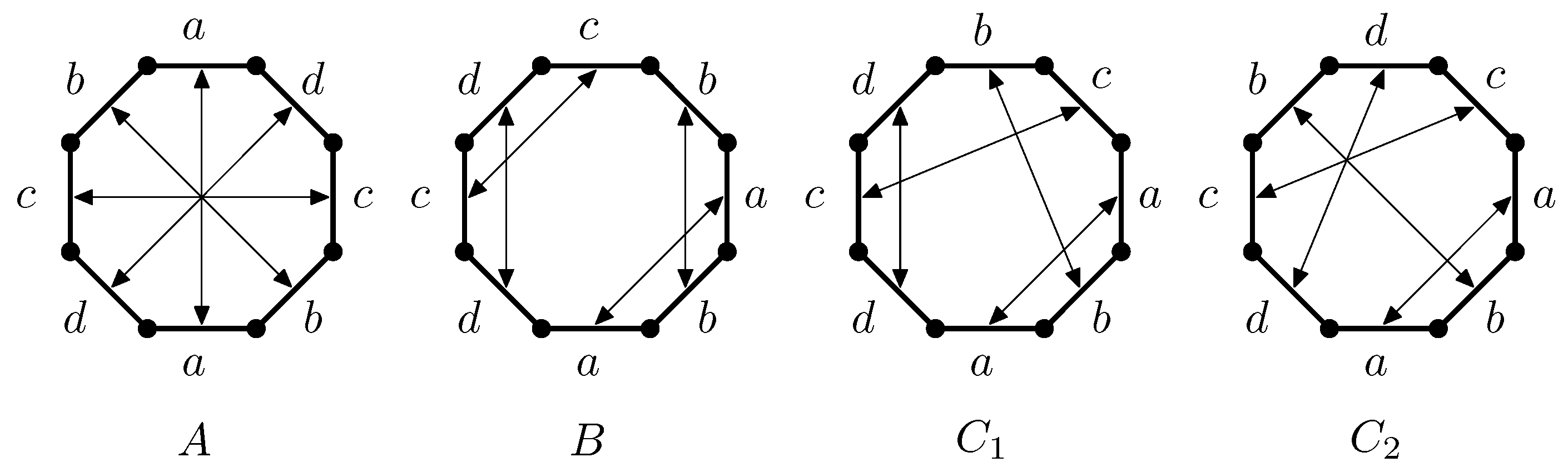
As we already know from [27], over $\mathbb{C}$, there are precisely four realizations of the above passport corresponding to the four possible ways of pasting the octagon (see Figure 2). The corresponding Gaussian words and the automorphism groups are presented in

Table 3. Gaussian words and automorphism groups.

Pasting	Gaussian Word	Aut
A	$abcdabcd$	cyclic of order 8
B	$ababcdcd$	cyclic of order 2
$C_1$	$abacbdcd$	trivial
$C_2$	$abacdbcd$	trivial

.

The completeness of our list can be checked by the Harer–Zagier numbers: introduce, following [28], the numbers

$${\epsilon }_g\left(n\right):=\#\left\{\mathrm{pastings}\mathrm{of}2n-\mathrm{gons}\mathrm{with}\mathrm{a}\mathrm{marked}\mathrm{edge}\mathrm{of}\mathrm{genus}g\right\}.$$

It is known that ${\epsilon }_2\left(4\right)=21$, and, indeed

$$21=8·\sum _{D\in \{A,B,C_1,C_2\}}\frac{1}{\#\mathrm{Aut}\left(D\right)}=8\left(\frac{1}{8}+\frac{1}{2}+1+1\right).$$

3.3.5. Some Qualitative Results

In this subsection, we denote the Belyi pairs corresponding to pastings by the Gaussian words defining pastings.

The certain properties of Belyi pairs follow immediately from the easy considerations in the category of dessins (Theorem 2).

Theorem 2.

(i) The Belyi pairs ${(\mathbf{X},\beta )}_{abcdabcd}$ and ${(\mathbf{X},\beta )}_{ababcdcd}$ are defined over $\mathbb{Q}$;

(ii) The remaining two, ${(\mathbf{X},\beta )}_{abacbdcd}$ and ${(\mathbf{X},\beta )}_{abacdbcd}$, are Galois-conjugated over some $\mathbb{Q}\left(\sqrt{D}\right)$ with $D>0$;

(iii) All the four Belyi pairs are self-dual, i.e., satisfy $(\mathbf{X},\beta )\cong (\mathbf{X},\frac{1}{\beta })$.

Proof. 

$\left(i\right)$ Both pairs ${(\mathbf{X},\beta )}_{abcdabcd}$ and ${(\mathbf{X},\beta )}_{ababcdcd}$ are defined uniquely by the triple invariants(degree, genus, Aut), so they are defined over $\mathbb{Q}$.

Before the actual calculations, the statement $\left(ii\right)$ is partially conjectural: from the known Galois-invariants, it follows that either ${(\mathbf{X},\beta )}_{abacbdcd}$ and ${(\mathbf{X},\beta )}_{abacdbcd}$ are also both defined over $\mathbb{Q}$ (separated by some finer Galois-invariants), or they constitute the two-element Galois orbit. The direct calculation will show below that the latter case holds, but we can already claim that the corresponding quadratic field of definition is real since ${(\mathbf{X},\beta )}_{abacbdcd}$ and ${(\mathbf{X},\beta )}_{abacdbcd}$ are not mutually mirror-symmetric.

The statement $\left(iii\right)$ follows from the self-duality of all the four pastings, which can be established by the direct pictorial analysis. □

As we have promised, we specify the terminology: from now on, we call the Belyi pairs ${(\mathbf{X},\beta )}_{abcdabcd}$ and ${(\mathbf{X},\beta )}_{ababcdcd}$ easy and ${(\mathbf{X},\beta )}_{abacbdcd}$ and ${(\mathbf{X},\beta )}_{abacdbcd}$ difficult (Remark 1).

Remark 1.

As we shall see, the difficult pairs are defined over $\mathbb{Q}\left(\sqrt{2}\right)$. It would be interesting to be able to determine the discriminant of the field of definition of a dessin without the calculation of the corresponding Belyi pair.

Restore some notations. Let $(\mathbf{X},\beta )$ be any of our four Belyi pairs. Then, according to the dessins d’enfants theory, since all our dessins have only one vertex and only one face, there exist such $A,C\in \mathbf{X}$ that

$$\mathrm{div}\left(\beta \right)=8A-8C,$$

hence

$$A-C\in {\mathrm{tors}}_8\left(\mathrm{Jac}\mathbf{X}\right).$$

Of course, the difference $A-C$ can actually have the smaller order in $\mathrm{Jac}\mathbf{X}$, and it turns out that all the possibilities realize—see the claim in [27].

Our terminology is reformulated in the following (Theorem 3)

Theorem 3.

In the above notations, the differences satisfy

$\left(i\right)$

$A-C\in {\mathrm{tors}}_2\left(\mathrm{Jac}{\mathbf{X}}_{abcdabcd}\right)$;

$\left(ii\right)$

$A-C\in {\mathrm{tors}}_4\left(\mathrm{Jac}{\mathbf{X}}_{ababcdcd}\right)\backslash {\mathrm{tors}}_2\left(\mathrm{Jac}{\mathbf{X}}_{ababcdcd}\right)$;

$\left(iii\right)$

in the difficult cases $A-C\in {\mathrm{tors}}_8\left(\mathrm{Jac}\mathbf{X}\right)\backslash {\mathrm{tors}}_4\left(\mathrm{Jac}\mathbf{X}\right)$.

Proof. 

Follows from the results below. The direct proofs in terms of dessins are also possible. □

3.3.6. Calculations

The easiest case ${\mathbf{X}}_{abcdabcd}$ has been covered before; the answer is

$$\begin{array}{|c|}\hline y^2=x^5-x,\beta =x^4\\ \hline\end{array}$$

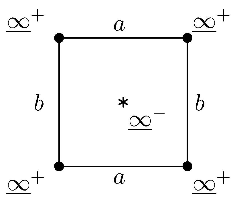
The easy case ${\mathbf{X}}_{ababcdcd}$. It follows from the symmetry considerations that there exists a degree-2 morphism of Belyi pairs

$$p:{\mathbf{X}}_{ababcdcd}⟶{\mathbf{Y}}_{abab},$$

where ${\mathbf{Y}}_{abab}$ is the toric dessin that is represented by a square with the opposite sides identified—see Figure 3 in which the vertices are marked in a way that will become clear in a while.

The Belyi pair $({\mathbf{Y}}_{abab},{\beta }_1)$, corresponding to this dessin, is determined immediately. There is only the elliptic curve with the symmetry of the 4th order; it has the j-invariant 1728. We take the doubly-dotted curve for its affine model

$$\ddot{\mathbf{Y}}:v^2=u^4-1$$

and understand it as

$$\ddot{\mathbf{Y}}={\mathbf{Y}}_{abab}\backslash \left\{{\underline{\infty }}^{\pm }\right\},$$

where around the points ${\underline{\infty }}^{\pm }$, the asymptotic $v\approx \pm u^2$ holds.

Now recall the notations $\mathrm{div}\left(\beta \right)=8A-8C$ and deduce from the geometry that

$$\beta =p^{*}{\beta }_1,$$

hence, assuming that the branching points of p are $p\left(A\right)={\underline{\infty }}^{+}$ and $p\left(C\right)={\underline{\infty }}^{-}$, we conclude that

$$\mathrm{div}\left({\beta }_1\right)=4{\underline{\infty }}^{+}-4{\underline{\infty }}^{-}.$$

Such a function turns out to be the square

$${\beta }_1=1-2u^4+2u^{2}v=-{(u^2-v)}^2.$$

Due to the identity $(u^2-v)(u^2+v)\equiv 1$, the polynomials $u^2\pm v$ are non-constant units of the polynomial ring of an affine curve. The subject is classical: N.-H. Abel was interested in such polynomials since they provide the pseudo-elliptic integrals (see [29]).

To provide the appropriate branching, introduce the correspondences (two-valued “functions”)

$$x=\sqrt{u+1},y=\frac{v}{\sqrt{u+1}}$$

which means introducing the affine model of ${\mathbf{X}}_{ababcdcd}$ by the equation

$$\begin{array}{|c|}\hline x^2{y}^2={(x^2-1)}^4-1\\ \hline\end{array}$$

together with the covering $p:{\mathbf{X}}_{ababcdcd}⟶{\mathbf{Y}}_{abab}$ defined by the pullbacks

$$p^{*}u=x^2-1,p^{*}v=xy.$$

The Belyi function is defined by $\beta =p^{*}{\beta }_1$, i.e.,

$$\begin{array}{|c|}\hline \beta =-{\left({(x^2-1)}^2-xy\right)}^2\\ \hline\end{array}$$

as we have asserted above, it is a square.

The boxed formulas are easily transformed to the answers of [27]:

$$\begin{array}{|c|}\hline y^2=x^6-4x^4+6x^2-4,\beta =-2x^8+8x^6-12x^4+8x^2-1+(2x^5-4x^3+2x)y\\ \hline\end{array}$$

However, the special properties of the considered dessin are not so easily seen in this standard form as in the above formulas.

The difficult cases ${\mathbf{X}}_{abacbdcd}$ and ${\mathbf{X}}_{abacbdcd}$. (The results are based on the computer calculation performed with the aid of S.Yu. Orevkov.) Due to the mentioned above self-duality, the desired Belyi pair is defined by the three recurrent polynomials. Namely, we consider the family of pairs $(\mathbf{X},\mathsf{\Psi })$, where $\mathbf{X}$ is a curve over an algebraically closed field and $\mathsf{\Psi }\in \mathbb{k}\left(\mathbf{X}\right)\backslash \mathbb{k}$. These pairs can be considered as the points of Hurwitz spaces. The affine model of where $\mathbf{X}$ is defined by the equation

$$y^2=a{x}^6+b{x}^5+c{x}^4+d{x}^3+c{x}^2+bx+a$$

(17)

and the function $\mathsf{\Psi }$ has the form

$$\mathsf{\Psi }=A{x}^8+B{x}^7+C{x}^6+D{x}^5+E{x}^4+D{x}^3+C{x}^2+Bx+A$$

$$+(F{x}^5+G{x}^4+H{x}^3+H{x}^2+Gx+F)y$$

(18)

Here, the parameters $(a:b:c:d)\in {\mathbf{P}}_3\left(\mathbb{k}\right),(A:B:C:D:E)\in {\mathbf{P}}_4\left(\mathbb{k}\right)$ and $(F:G:H)\in {\mathbf{P}}_2\left(\mathbb{k}\right)$ are defined up to proportionality and satisfy

$$aAF\ne 0,$$

so we could normalize the coefficients of the pair $(\mathbf{X},\mathsf{\Psi })$ by $a=A=F=1$ and look for the desired points (recall that there are two of them defined over the yet unknown quadratic extension of $\mathbb{Q}$) in the affine space ${\mathbf{A}}_9\left(\mathbb{k}\right)$. However, then the arithmetical issues occur, so we prefer to keep our 12 unknown parameters $a,\dots ,H$ free. The resulting family of curves over ${\mathbf{P}}_3\left(\mathbb{k}\right)$ with rational functions parametrized by the points of ${\mathbf{P}}_4\left(\mathbb{k}\right)\times {\mathbf{P}}_2\left(\mathbb{k}\right)$ is interesting for its own reason; we are looking for the two very special fibers in this family. See the general discussion in [30].

The points ${\mathrm{O}}^{\pm }\in \mathbf{X}$ and ${\underline{\infty }}^{\pm }\in \mathbf{X}$ are defined by

$$\left(x\left({\mathrm{O}}^{\pm }\right)=0,y\left({\mathrm{O}}^{\pm }\right)=\pm \sqrt{a}\right)\mathrm{and}\left(x\left({\underline{\infty }}^{\pm }\right)=0,y\approx \pm \sqrt{a}{x}^3\right)\mathrm{as}x\to \infty .$$

(The choice of signs motivated by arithmetics). We are looking for the pairs $(\mathbf{X},\mathsf{\Psi })$ satisfying

$$\mathrm{div}\left(\mathsf{\Psi }\right)=8\mathrm{O}-8\underline{\infty }.$$

(19)

after the appropriate choices $\mathrm{O}\in \left\{{\mathrm{O}}^{\pm }\right\},\underline{\infty }\in \left\{{\underline{\infty }}^{\pm }\right\}$. (They are opposite by the geometric reasons; we do not discuss them here.)

After solving Equation (18) in y and plugging the result in (17), we obtain the condition for a recurrent polynomial

$$\mathcal{Z}=z_0{x}^{16}+z_1{x}^{15}+\dots +z_7{x}^9+z_8{x}^8+z_7{x}^7+\dots z_{1}x+z_0\in \mathbb{k}[x,\mathsf{\Psi }],$$

(20)

for which Equation (19) is equivalent to

$$\mathcal{Z}{|}_{\mathsf{\Psi }=0}\in {\mathbb{k}}^{\times }[a,\dots ,H]x^8,$$

or to the system of polynomial equations

$$z_0=z_1=\dots =0$$

that we rewrite in the polynomial form

$$(2F^{2}c+2FGa+2FGb+2FGd+2FHa+2FHb+2FHc+G^{2}b+2G^{2}c+2GHa$$

$$+2GHb+2GHc+2GHd+H^{2}b+2H^{2}c+H^{2}d-2AB-2BC-2CD-2DE)x^7$$

$$+(F^{2}a+2F^{2}b+2FGa+2FGb+2FGc+2FHc+2FHd+2G^{2}b+G^{2}c+2GHa$$

$$+2GHc+2GHd+H^{2}a+2H^{2}b+H^{2}c-2AC-2BD-2CE-D^2)x^6$$

$$+(2F^{2}a+F^{2}b+2FGb+2FGc+2FHc+2FHd+2G^{2}a+G^{2}d$$

$$+2GHb+2GHc+2H^{2}a+H^{2}b-2AD-2BE-2CD)x^5$$

$$+(F^{2}c+2FGa+2FGd+2FHb+2FHc+G^{2}c$$

$$+2GHa+2GHb+H^{2}a-2AE-2BD-C^2)x^4$$

$$+(F^{2}d+2FGc+2FHa+2FHb+G^{2}b+2GHa-2AD-2BC)x^3$$

$$+(F^{2}c+2FGb+2FHa+G^{2}a-2AC-B^2)x^2$$

$$+(F^{2}b+2FGa-2AB)x$$

$$+F^{2}a-A^2\equiv 0.$$

(21)

The coefficients of the equation of the curve are eliminated straightforwardly

$$a=\frac{A^2}{F^2},b=-\frac{2A(AG-BF)}{F^3},$$

$$c=-\frac{2A^{2}FH-3A^2{G}^2+4ABFG-2AC{F}^2-B^2{F}^2}{F^4},$$

$$d=-\frac{2}{F^5}(A^2{F}^{2}H-3A^{2}FGH+2A^2{G}^3+2AB{F}^{2}H-3ABF{G}^2$$

$$+2AC{F}^{2}G-AD{F}^3+B^2{F}^{2}G-BC{F}^3)$$

(22)

leaving us with the system of four equations in polynomial form

$$(2A^2{F}^{4}G-2A^2{F}^{4}H+2A^2{F}^3{G}^2-6A^2{F}^{3}GH-4A^2{F}^3{H}^2-2A^2{F}^2{G}^3$$

$$+10A^2{F}^2{G}^{2}H-10A^2{F}^{2}G{H}^2-6A^2{F}^2{H}^3-2A^{2}F{G}^4+6A^{2}F{G}^{3}H$$

$$+18A^{2}F{G}^2{H}^2+6A^{2}FG{H}^3-8A^2{G}^{4}H-4A^2{G}^3{H}^2-2AB{F}^5$$

$$-4AB{F}^{4}G+4AB{F}^{4}H+2AB{F}^3{G}^2-12AB{F}^{3}GH+2AB{F}^3{H}^2$$

$$+4AB{F}^2{G}^3-8AB{F}^2{G}^{2}H-16AB{F}^{2}G{H}^2-4AB{F}^2{H}^3$$

$$+12ABF{G}^{3}H+6ABF{G}^2{H}^2+4AC{F}^5+4AC{F}^{4}H-4AC{F}^3{G}^2$$

$$+4AC{F}^{3}GH+4AC{F}^3{H}^2-8AC{F}^2{G}^{2}H-4AC{F}^{2}G{H}^2$$

$$+4AD{F}^{4}G+4AD{F}^{3}GH+2AD{F}^3{H}^2+2B^2{F}^5+2B^2{F}^{4}H-2B^2{F}^3{G}^2$$

$$+2B^2{F}^{3}GH+2B^2{F}^3{H}^2-4B^2{F}^2{G}^{2}H-2B^2{F}^{2}G{H}^2-2BC{F}^5$$

$$+4BC{F}^{4}G+4BC{F}^{3}GH+2BC{F}^3{H}^2-2CD{F}^5-2DE{F}^5)x^7$$

$$+(A^2{F}^5-2A^2{F}^{4}G-4A^2{F}^3{G}^2-2A^2{F}^{3}GH-7A^2{F}^3{H}^2+2A^2{F}^2{G}^3$$

$$+4A^2{F}^2{G}^{2}H-2A^2{F}^2{H}^3+3A^{2}F{G}^4-2A^{2}F{G}^{3}H+15A^{2}F{G}^2{H}^2$$

$$-8A^2{G}^{4}H+4AB{F}^5+4AB{F}^{4}G-4AB{F}^3{G}^2-8AB{F}^{3}GH$$

$$-4AB{F}^3{H}^2-4AB{F}^2{G}^3+4AB{F}^2{G}^{2}H-12AB{F}^{2}G{H}^2+12ABF{G}^{3}H$$

$$-2AC{F}^5+4AC{F}^{4}G+4AC{F}^{4}H+2AC{F}^3{G}^2-4AC{F}^{3}GH$$

$$+2AC{F}^3{H}^2-8AC{F}^2{G}^{2}H+4AD{F}^{4}H+4AD{F}^{3}GH+2B^2{F}^{4}G$$

$$+2B^2{F}^{4}H+B^2{F}^3{G}^2-2B^2{F}^{3}GH+B^2{F}^3{H}^2-4B^2{F}^2{G}^{2}H$$

$$+4BC{F}^{4}H+4BC{F}^{3}GH-2BD{F}^5-2CE{F}^5-D^2{F}^5)x^6$$

$$+(2A^2{F}^5-2A^2{F}^{4}G-2A^2{F}^3{G}^2-4A^2{F}^{3}GH-6A^2{F}^3{H}^2$$

$$+6A^2{F}^2{G}^3+6A^2{F}^{2}G{H}^2+4A^{2}F{G}^{3}H-4A^2{G}^5+2AB{F}^5$$

$$+4AB{F}^{4}G-8AB{F}^3{G}^2-4AB{F}^{3}GH-6AB{F}^3{H}^2+6ABF{G}^4$$

$$+4AC{F}^{4}G+4AC{F}^{4}H-4AC{F}^{3}GH-4AC{F}^2{G}^3-2AD{F}^5$$

$$+4AD{F}^{4}H+2AD{F}^3{G}^2+2B^2{F}^{4}G+2B^2{F}^{4}H-2B^2{F}^{3}GH$$

$$-2B^2{F}^2{G}^3+4BC{F}^{4}H+2BC{F}^3{G}^2-2BE{F}^5-2CD{F}^5)x^5$$

$$+(2A^2{F}^{4}G-2A^2{F}^{4}H+3A^2{F}^3{G}^2-6A^2{F}^{3}GH-3A^2{F}^3{H}^2$$

$$+12A^2{F}^2{G}^{2}H-5A^{2}F{G}^4-4AB{F}^{4}G+4AB{F}^{4}H-12AB{F}^{3}GH$$

$$+8AB{F}^2{G}^3+2AC{F}^5+4AC{F}^{4}H-6AC{F}^3{G}^2+4AD{F}^{4}G$$

$$-2AE{F}^5+B^2{F}^5+2B^2{F}^{4}H-3B^2{F}^3{G}^2+4BC{F}^{4}G$$

$$-2BD{F}^5-C^2{F}^5)x^4\equiv 0.$$

(23)

These equations admit the straightforward elimination of D and E and then become really terrible. However, they imply the quadratic equation in A:

$$(20F^4+48F^{3}G-16F^{3}H-4F^2{G}^2-8F^{2}GH+4F^2{H}^2-40F{G}^3+40F{G}^{2}H-8G^4)A^2$$

$$+(-30B{F}^4-2B{F}^{3}G+4B{F}^{3}H+54B{F}^2{G}^2-52B{F}^{2}GH+10BF{G}^3)A$$

$$+5B^2{F}^4-18B^2{F}^{3}G+16B^2{F}^{3}H-3B^2{F}^2{G}^2,$$

fortunately, with the nice discriminant

$$4{(5F^2+2FG-4FH+G^2)}^3{B}^2{F}^2.$$

In order to make this discriminant a square, we introduce the new variable $\Delta$ by the relation

$$\begin{array}{|c|}\hline {\Delta }^2=5F^2+2FG-4FH+G^2\\ \hline\end{array}$$

(24)

and eliminate two unknowns:

$$H=-\frac{1}{4}\frac{{\Delta }^2-5F^2-2FG-G^2}{F}$$

(25)

and

$$B=\frac{A}{2}·\frac{{\Delta }^2-2\Delta F-6\Delta G+5F^2+14FG-3G^2}{(5F-G-2\Delta )F}$$

(26)

Introducing the new variable

$$\begin{array}{|c|}\hline \delta :=-5F+G+2\Delta \\ \hline\end{array}$$

(27)

yields the family of curves over the projective space ${\mathbf{P}}_3\left(\mathbb{k}\right)=\left\{(\Delta :\delta :A:F)\right\}$, among which the desired two are:

$$a=\frac{A^2}{F^2},b=-\frac{A^2\left({\Delta }^2+2\Delta \delta -6F\delta -{\delta }^2\right)}{F^3\delta },$$

$$c=\frac{1}{4}\frac{A^2{\Delta }^4+8{\Delta }^3\delta -16{\Delta }^{2}F\delta -2{\Delta }^2{\delta }^2-32\Delta F{\delta }^2-4\Delta {\delta }^3+60F^2{\delta }^2+16F{\delta }^3+{\delta }^4}{F^4{\delta }^2},$$

$$d=\frac{A^2}{F^5{\delta }^2}({\Delta }^5-{\Delta }^{4}F-8{\Delta }^{3}F\delta -{\Delta }^3{\delta }^2+12{\Delta }^2{F}^2\delta +2{\Delta }^{2}F{\delta }^2$$

$$+24\Delta F^2{\delta }^2+4\Delta F{\delta }^3-40F^3{\delta }^2-12F^2{\delta }^3-F{\delta }^4).$$

(28)

The desired behavior of $\mathsf{\Psi }$ defines a highly reducible surface in ${\mathbf{P}}_3\left(\mathbb{k}\right)$, from which we select the needed component

$$F=\frac{1}{2}\Delta .$$

(29)

Equation (17) over this component factorizes:

$$\begin{array}{|c|}\hline \frac{{\Delta }^4{\delta }^2{y}^2}{4A^2}=\left(\delta x^2-(\Delta -\delta )x+\Delta \right)\left(\Delta x^2-(\Delta -\delta )x+\delta \right)\left(\Delta \delta x^2-({\Delta }^2-2\Delta \delta -{\delta }^2)x+\Delta \delta \right)\\ \hline\end{array}$$

(30)

Choose the scaling factor in such a way that the equation

$$y^2=\left(\delta x^2-(\Delta -\delta )x+\Delta \right)\left(\Delta x^2-(\Delta -\delta )x+\delta \right)\left(\Delta \delta x^2-({\Delta }^2-2\Delta \delta -{\delta }^2)x+\Delta \delta \right)$$

(31)

holds.

The appropriate behavior of the critical values of $\mathsf{\Psi }$ takes place over the hyperbola

$$\begin{array}{|c|}\hline \Delta \delta =7\\ \hline\end{array}$$

(32)

over which Equation (31) takes the form (note that the curve is terribly degenerate over ${\mathbb{F}}_7$; for the time being, the authors have no complete explanation).

$$y^2=({\delta }^2{x}^2+{\delta }^{2}x-7x+7)\left(7x^2+({\delta }^2-7)x+{\delta }^2\right)\left(7{\delta }^2{x}^2+({\delta }^4+14{\delta }^2-49)x+7{\delta }^2\right)$$

(33)

The right-hand side of (33) depends only on ${\delta }^2$, and the values we look for are over the conjugated quadratic irrationalities

$$\begin{array}{|c|}\hline {\delta }^2=-7\pm 7\sqrt{2}\\ \hline\end{array}$$

(34)

Over these points, finally, our two curves are defined by the equation

$$\begin{array}{|c|}\hline y^2=\left(x^2-(2\pm \sqrt{2})x\mp \sqrt{2}-1\right)(x^2\pm \sqrt{2}x+1\mp \sqrt{2})(x^2+1)\\ \hline\end{array}$$

(35)

The Belyi functions are not so nice. We present them in the form

$$-4(1\pm \sqrt{2})\beta =M+Ny$$

with the two recurrent polynomials

$$M=x^8-(2\pm 2\sqrt{2})x^7+2x^6+(6\pm 2\sqrt{2})x^5-(2\pm 4\sqrt{2})x^4$$

$$+(6\pm 2\sqrt{2})x^3+2x^2-(2\pm 2\sqrt{2})x+1$$

and

$$N=x^5-(1\pm 2\sqrt{2})x^4+2x^3+2x^2-(1\pm 2\sqrt{2})x+1.$$

The alternative form:

$$N=\left(x^2-(2\pm \sqrt{2})x+1\right)(x^2\mp \sqrt{2}x-1)(x+1)$$

The abscissas of the points in which $\beta =1$ are defined by the equation

$$(x^2+1){(x+1)}^2{(x^2\mp \sqrt{2}x+1)}^2=0.$$

4. Conclusions

It is not immediately clear that the intensive computer calculation of Belyi pairs with the incredibly complicated answers really provides a better understanding of the relation between combinatorial topology and arithmetic geometry. For example, though we can see some Galois orbits now, the inverse Galois problem is as out of reach as it was forty years ago.

However, some motivation for these calculations can be drawn from the historic perspectives. For example, our understanding of the polynomial equations was preceded by the period, when finding roots meant their explicit expression in terms of the coefficients. A similar attitude to the relations between the dessins and Belyi pairs is dominating now: seeing a dessin, the experts usually want to calculate the corresponding Belyi pair; the ability to understand the underlying arithmetic without such a calculation is in its infancy. Similar parallels can be drawn in calculus, differential equations, etc.

However, living today, we can only dream about the future understanding of the phenomena attracting us—as, maybe, Cardano could dream about knowing the number of roots of any univariate polynomials. Our modest goal is not only to leave some ideas and problems to future generations but also to provide some systematized material. Happily, the computers around us empower the interested mathematicians to reach the results totally impossible by hand calculations.

Complete lists of Belyi pairs of the bounded complexity constitute examples of such material. The results of the present paper correspond to a very low bound (basically ≤ four edges). However, they contain some evidence crying out for a conceptual explanation – e.g., lots of enigmatic coincidences and unpredictable simplifications. The authors hope to improve the current understanding and to present the same results in a clearer form.

References

- Tutte, W.T. What is a map? In New Directions in the Theory of Graphs; Harary, F., Ed.; Academic Press: New York, NY, USA, 1973. [Google Scholar]
- Harary, F.; Palmer, E.M. Graphical Enumeration; Academic Press: Cambridge, MA, USA, 1973. [Google Scholar]
- Bose, S.; Gundry, J.; He, Y.-H. Gauge theories and dessins d’enfants: Beyond the torus. J. High Energy Phys. 2015, 2015, 135. [Google Scholar] [CrossRef]
- Asselmeyer-Maluga, T. Quantum computing and the brain: Quantum nets, dessins d’enfants and neural networks. In Proceedings of the Quantum Technology International Conference 2018, Paris, France, 5–7 September 2018; Volume 198, p. 00014. [Google Scholar]
- Artin, M.; Jackson, A.; Mumford, D.; Tate, J. Alexandre Grothendieck 1928–2014, Part 1. Not. AMS 2016, 63, 242–255. [Google Scholar]
- Belyi, G.V. Galois extensions of a maximal cyclotomic fields. Math. USSR Izv. 1980, 14, 247–256. [Google Scholar] [CrossRef]
- Schneps, L. Dessins d’enfants on the Riemann sphere. In The Grothendieck Theory of Dessins d’Enfants; Schneps, L., Ed.; London Mathematical Society Lecture Note Series; Cambridge University Press: Cambridge, UK, 1994; Volume 200, pp. 47–78. [Google Scholar]
- Musty, M.; Schiavone, S.; Sijsling, J.; Voight, J. A database of Belyi maps. In The Open Book Series 2, Thirteenth Algorithmic Number Theory Symposium; Mathematical Sciences Publishers: Berkeley, CA, USA, 2019. [Google Scholar]
- Grothendieck, A. Esquisse d’un Programme, Unpublished manuscript (1984). In Geometric Galois Actions; Lochak, P.; Schneps, L., Translators; London Mathematical Society Lecture Note Series; Cambridge University Press: Cambridge, UK, 1997; Volume 242, pp. 5–48. [Google Scholar]
- Shabat, G.B.; Voevodsky, V.A. Drawing Curves Over Number Fields. In The Grothendieck Festschrift: Progress in Mathematics; Cartier, P., Illusie, L., Katz, N.M., Laumon, G., Manin, Y.I., Ribet, K.A., Eds.; Birkhäuser: Boston, MA, USA, 1990; Volume 88. [Google Scholar]
- Girondo, E.; Gonzalez-Diez, G. Introduction to Compact Riemann Surfaces and Dessins d’Enfants; London Mathematical Society Student Texts; Cambridge University Press: Cambridge, UK, 2012. [Google Scholar]
- Lando, S.; Zvonkin, A. Graphs on Surfaces and Their Applications; Springer: Berlin/Heidelberg, Germany, 2004. [Google Scholar]
- Sijsling, J.; Voight, J. On computing Belyi maps. Publications Mathématiques de Besançon Algèbre et Théorie des Nombres 2014, 1, 73–131. [Google Scholar] [CrossRef] [Green Version]
- Shabat, G. Calculating and drawing Belyi pairs. J. Math. Sci. 2017, 226, 667–693. [Google Scholar] [CrossRef]
- Adrianov, N.M.; Amburg, N.Y.; Dremov, V.A.; Kochetkov, Y.Y.; Kreines, E.M.; Levitskaya, Y.A.; Nasretdinova, V.F.; Shabat, G.B. Catalog of dessins d’enfants with no more than 4 edges. J. Math. Sci. 2009, 158, 22–80. [Google Scholar] [CrossRef] [Green Version]
- Shabat, G.B.; Zvonkin, A.K. Plane trees and algebraic numbers. In Contemporary Mathematics, Proceedings of the “Jerusalem Combinatorics’ 93”, Jerusalem, Israel, 9–17 May 1993; AMS: Jerusalem, Israel, 1994; Volume 176, pp. 233–275. [Google Scholar]
- Bétréma, J.; Péré, D.; Zvonkin, A.K. Plane Trees and Their Shabat Polynomials; Rapport Interne du LaBRI: Bordeaux, France, 1992. [Google Scholar]
- Kochetkov, Y.Y. Plane trees with nine edges. Catalog. J. Math. Sci. 2009, 158, 114–140. [Google Scholar] [CrossRef]
- Kochetkov, Y.Y. Short catalog of plane ten-edge trees. arXiv 2014, arXiv:1412.2472v1. [Google Scholar]
- Adrianov, N.M.; Kochetkov, Y.Y.; Suvorov, A.D.; Shabat, G.B. Mathieu groups and plane trees. Fundam. Prikl. Mat. 1995, 1, 377–384. [Google Scholar]
- Shabat, G. Unicellular four-edged toric dessins. J. Math. Sci. 2015, 209, 309–318. [Google Scholar] [CrossRef]
- Goupil, A.; Schaeffer, G. Factoring N-cycles and counting maps of given genus. Eur. J. Comb. 1998, 19, 819–834. [Google Scholar] [CrossRef] [Green Version]
- Dremov, V.A. Is 1 − β a square? Unpublished. 2000. [Google Scholar]
- Igusa, J. On Siegel modular forms of genus two. Am. J. Math. 1962, 84, 175–200. [Google Scholar] [CrossRef]
- Birch, B. Non-congruence subgroups, covers and drawings. In The Grothendieck Theory of Dessins D’Enfants; London Mathematical Society Lecture Note Series; Cambridge University Press: Cambridge, UK, 1994; Volume 200, pp. 25–46. [Google Scholar]
- Fuertes, Y.; Mednykh, A. Genus 2 semi-regular coverings with lifting symmetries. Glasg. Math. J. 2008, 50, 379–394. [Google Scholar]
- Adrianov, N.M.; Shabat, G.B. Belyi functions of dessins d’enfants of genus 2 with 4 edges. Russ. Math. Surv. 2005, 60, 1237–1239. [Google Scholar] [CrossRef]
- Harer, J.; Zagier, D. The Euler characteristic of the moduli space of curves. Invent. Math. 1986, 85, 457–485. [Google Scholar] [CrossRef] [Green Version]
- Abel, N.-H. Sur l’intégration de la formule différentielle , R et ρ étant des fonctions entières. J. Reine Angew. Math. 1826, 1, 185–221. [Google Scholar]
- Shabat, G. Belyi pairs in the critical filtrations of Hurwitz spaces. In Teichmüller Theory and Grothendieck-Teichmüller Theory; Ji, L., Papadopoulos, A., Su, W., Eds.; Advanced Lectures in Mathematics (ALM); International Press: Somerville, MA, USA, 2022; pp. 320–341. [Google Scholar]
Figure 1.
Unicellular dessins of genus 1 with 4 edges.
Figure 2.
Octagon pastings of genus 2.