
Prediction of Airfoil Stall Based on a Modified

School of Aerospace Engineering, Tsinghua University, Beijing 100084, China
*
Author to whom correspondence should be addressed.
Mathematics 2022, 10(2), 272; https://0-doi-org.brum.beds.ac.uk/10.3390/math10020272
Submission received: 15 December 2021
/
Revised: 10 January 2022
/
Accepted: 14 January 2022
/
Published: 16 January 2022
(This article belongs to the Special Issue Advances in Computational Fluid Dynamics)
Abstract
:The accuracy of an airfoil stall prediction heavily depends on the computation of the separated shear layer. Capturing the strong non-equilibrium turbulence in the shear layer is crucial for the accuracy of a stall prediction. In this paper, different Reynolds-averaged Navier–Stokes turbulence models are adopted and compared for airfoil stall prediction. The results show that the separated shear layer fixed (abbreviated as SPF ) turbulence model captures the non-equilibrium turbulence in the separated shear layer well and gives satisfactory predictions of both thin-airfoil stall and trailing-edge stall. At small Reynolds numbers (), the relative error between the predicted of NACA64A010 by the SPF model and the experimental data is less than 3.5%. At high Reynolds numbers (), the of NACA64A010 and NACA64A006 predicted by the SPF model also has an error of less than 5.5% relative to the experimental data. The stall of the NACA0012 airfoil, which features trailing-edge stall, is also computed by the SPF model. The SPF model is also applied to a NACA0012 airfoil, which features trailing-edge stall and an error of relative to the experiment at is smaller than 3.5%. The SPF model shows higher accuracy than other turbulence models.
1. Introduction
The stall phenomenon often appears in airplane wings and empennages, compressor blades and helicopter rotors [1]. The stall of the main wing can cause the aircraft to lose lift. Flow separation associated with stall can compromise control surface performance or even make an aircraft uncontrollable. The aerodynamic performance of a deeply stalled airfoil (i.e., airfoil operating at angles of attack larger than the stall angle of attack ) is also important in some applications, such as rotorcraft [2,3] and wind turbines. Consequently, the characteristics of the airfoil stall must be accurately predicted in aerodynamic design.
The stalling characteristics of airfoils have been widely studied experimentally. McCullough and Gault [4] conducted detailed wind tunnel tests and classified airfoil stalls into three types: trailing-edge stall, leading-edge stall and thin-airfoil stall. The locations and evolution of separation bubbles are different for each stall type. Trailing-edge stall is preceded by the turbulent boundary layer separation point gradually moving forward as the angle of attack increases. This movement eventually results in a mild loss of the lift coefficient beyond . Leading-edge stall results from the burst of a laminar separation bubble that has formed near the leading edge of the airfoil. When increases, the flow separates from the upper surface of the airfoil abruptly and causes a sharp loss in the lift. In a thin-airfoil stall, a laminar separation bubble forms at the leading edge, and the airfoil stall is preceded by the gradual growth of the separation bubble as the angle of attack increases. Bragg [5] experimentally studied the stalling characteristics of NACA64A010 and found that the airfoil exhibited thin-airfoil stall features. At , the slope of the curve decreased significantly. Bragg attributed the loss in slope to the appearance of a leading-edge separation bubble at . Tani [6] suggested that this is because the short separation bubble becomes a long bubble. At , the lift coefficient attained its maximum and started to decrease. At , the lift started to recover, and bluff body vortex shedding was observed by Bragg [5].
Accurate numerical simulation of airfoil stall is challenging. Complex phenomena, including an adverse pressure gradient, boundary layer separation and transition, are involved in the flow past a stalled airfoil [7]. Many unsteady simulations have numerically predicted airfoil stall performance. Rodriguez et al. [8] conducted a direct numerical simulation (DNS) study to learn the flow details around the NACA0012 airfoil at a large angle of attack. The results showed that the flow had three main characteristics: boundary layer separation at the leading edge, Kelvin–Helmholtz (K-H) instability in the separated shear layer, which eventually leads to transition, and large eddies, which induce strong momentum exchange after the transition point. Mary and Sagaut [9] conducted a large eddy simulation (LES) of the turbulent flow past an A-Airfoil. This study showed that LES could give relatively accurate results for the velocity profiles and the pressure distribution at large . At , the velocity profiles given by LES at reflected the flow separation successfully and differed from the experimental data by only 5%. Additionally, the relative error of the computed pressure coefficient and experimental data under the separation bubble () was less than 5%. Im and Zha [10] used a delayed, detached eddy simulation (DDES) with the Spalart–Allmaras turbulence model to predict the force coefficient of the NACA0012 airfoil. The lift coefficient and the drag coefficient were accurately predicted at angles of attack up to . Kawai and Fujii [11] also used the Reynolds-averaged Navier–Stokes/large eddy simulation (RANS/LES) hybrid method to simulate the flow past the NACA64A006 airfoil at up to . These unsteady simulations successfully predicted the growth of the laminar separation bubble. The results of the high-fidelity unsteady simulation methods were reported to be satisfactory. However, the large computational cost makes these methods unsuitable for the daily design process.
Currently, the steady Reynolds-averaged Navier–Stokes (RANS) method is widely used in practical engineering. The computational cost of the RANS method is relatively low, and it can provide an acceptable force coefficient at a small angle of attack. Although the flow past a stalled airfoil is essentially unsteady, using the steady RANS method to obtain a relatively accurate lift coefficient or other averaged features of the flow field is still quite desirable for daily aerodynamic design. The turbulence model should be used in the RANS method to approximate the unclosed Reynolds stress in the averaged Navier–Stokes equations. Two of the most commonly used turbulence models for aeronautics applications are the SST turbulence model and the SA turbulence model. The SST turbulence model gives accurate results in the near-wall layers. The zonal formulation based on blending functions makes the model insensitive to the free stream value. The SST turbulence model gives a relatively accurate separation point, but it underpredicts the level of turbulence stresses in the separated shear layer. The position of reattachment also disagrees with the experimental data [12]. The SA turbulence model contains a single PDE. Consequently, it is easy to implement the SA turbulence model in the existing code. The SA turbulence model is also proven to be numerically well behaved. The single PDE of the SA turbulence model can be applied to both incompressible and compressible flow, which makes it convenient for aeronautic applications of a wide speed range. However, the model uses a prescribed turbulence scale. This simplification compromises the model’s ability to predict the separated flow [13]. In Section 3 of this paper, the SST and SA model are used to predict the airfoil stall. The results show that their ability in stall prediction is limited.
Indeed, most RANS turbulence models have poor performance in predicting airfoil stalling characteristics. Rizzetta and Visbal [14] applied the Baldwin–Lomax algebraic model and two-equation model to compute the stall performance of the Sikorsky SSC-A09 airfoil and found that both models gave poor results. Genç [15] used the shear–stress transport (SST) model to simulate the stalling characteristics of the NACA64A006 airfoil and found that the model seriously underpredicted the lift coefficient when was large.
RANS methods with transition prediction may more accurately evaluate the airfoil’s stalling characteristics. Catalano and Tognaccini [16] developed an empirical method based on the analysis of the laminar separation bubble to approximate the transition point on an airfoil. The RANS simulation using a fixed transition point obtained by the empirical method gave satisfactory stall prediction of the SD7003 airfoil. Wokoeck et al. [17] introduced a transition prediction based on linear stability theory to RANS simulation and successfully predicted the laminar separation bubble on an airfoil surface. However, the maximum lift and the stalling angle of attack were not accurately computed. Genç [15] applied the transitional model [18,19,20] to predict the stalling characteristics of the NACA64A006 airfoil. The results showed that the size of the laminar separation bubble at small angles of attack agreed well with the experimental results. Morgado et al. [21] used the same transitional model to simulate the stall of E387 and S1223 airfoils. The results showed that the model could give a promising prediction of at large , provided that the were less than . In Section 3, an alternative version of the transitional model, called the model [20], is used to simulate the airfoil stall. The model and the model have similar characteristics.
Nearly all turbulence models mentioned above are calibrated by wall-bounded flow without massive flow separation. The lack of calibration by the separated flow leads to poor capability in predicting massive separation in the flow past an airfoil operating at . Rumsey [22] proposed that most RANS turbulence models underpredict the eddy viscosity in the shear layer region of a separation bubble and thus lead to insufficient mixing and delayed reattachment after flow separation. On the other hand, the non-equilibrium turbulence (which is characterized by a large ratio between the rates of turbulence kinetic energy production and the rates of dissipation) is prominent in the region of flow separation, where the adverse pressure gradient is strong [23]. In the research conducted by Fang [24,25], it was also found that the non-equilibrium turbulence appears in the separated shear layer. Based on these observations, Rumsey [26] developed a modified model, which recognizes the shear layer region by its high , enhances the destruction of in this region and produces a large eddy viscosity in the separated shear layer. This modification substantially improves the turbulence model’s ability to predict massive separation in some cases, such as the flow past a bump [26]. Li et al. [27,28,29] used a similar non-equilibrium modification function to improve the SST, and Wilcox 2006 models. The fixed term in these modified models, based on the non-equilibrium features of turbulence, can augment the eddy viscosity in the region where the non-equilibrium turbulence and the shear are strong. The improved model is called the separated shear layer fixed model. The separated shear layer fixed model successfully predicted the non-equilibrium turbulence in the separated shear layer produced by the ice accretion at the leading edge of the airfoil. The size of the separation bubble behind the ice corn also agreed well with the experiment. Zhang et al. [30] applied the separated shear layer fixed model to study the multi-element airfoils and a complex three-dimensional JAXA standard model with high-lift devices. The results showed that the separated shear layer fixed model performed well in predicting the separation bubble in the flow field. The lift coefficients of the multi-element airfoils and the three-dimensional JAXA standard model also agreed with the experiment results.
To summarize, the airfoil stall is an important phenomenon in wing design and turbine blade design. The stall performance is critical to the overall performance of an aircraft. An efficient method to predict airfoil stall is highly desirable. However, current high-fidelity methods (DNS and LES) are inefficient. RANS is significantly cheaper, but the mediocre performance of traditional turbulence models in separation flow prediction limits RANS’s application in stall prediction. The facts listed above motivated the authors to develop a turbulence model that is capable of stall prediction to serve for daily engineering design.
The authors believe that the SPF model has great potential in stall prediction, in which the separated shear layer plays an important role. In this paper, the separated shear layer fixed model’s (SPF model) ability to simulate airfoil stall is verified. The model is applied to several airfoil stall cases, including the thin-airfoil stall of the NACA64A010 airfoil at both low and high Reynolds numbers, thin-airfoil stall of the NACA64A006 airfoil and trailing-edge stall of the NACA0012 airfoil. The results of the test cases show that the SPF model performs better than traditional turbulence models in predicting the stall characteristics of different airfoil stall types. In thin-airfoil stall and trailing-edge stall, the separated shear layer where the non-equilibrium turbulence is strong develops and plays an important role in determining the lift coefficient of the airfoil. Since the modification term in the SPF model is aimed at the separated shear layer, the test cases contain both airfoils exhibiting thin-airfoil stall (NACA64A006 and NACA64A010) and airfoils exhibiting trailing-edge stall (NACA0012). These specific airfoils (NACA64A006, NACA64A010 and NACA0012) are chosen because their experimental data are relatively abundant in the current literature.
The authors believe that the SPF model can be used to evaluate the stall performance of a newly designed airfoil and can also be used to conduct numerical optimization of airfoils, for which the stall performance is important.
2. Governing Equations and Numerical Method
2.1. The Reynolds-Averaged Navier–Stokes Equations
Direct numerical simulation of fluid flow using Navier–Stokes equations is numerically expensive or even prohibitive due to the strong fluctuation and the multiple scales of turbulence. Averaging can be applied to Navier–Stokes equations to reduce the cost of simulation. The Reynolds-averaged equations can be written as follows [31]. Note that in all equations listed in this paper, the summation convention is used:
where are constants and
All variables with a bar denote averaged variables. The vector describes the heat diffusion caused by turbulent motion. The stress tensor in Equations (2) and (3) can be written as
where denotes the fluctuation velocity, which is the difference between the instantaneous velocity and the averaged velocity:
After substituting Equations (4) and (5) into Equations (2) and (3), one can find that there are 11 dependent variables. (The vector has 3 components, and the symmetric tensor called Reynolds stress tensor has 6 components.):
whereas there are only five partial differential equations in Equations (1)–(3). Consequently, the averaged Navier–Stokes equations are unclosed. To reduce the number of dependent variables, people use the Boussinesq approximation to express :
Equation (8) is an analog of the first two terms on the right-hand side of Equation (6). Physically speaking, the approximation in Equation (8) implies that the mechanism of the momentum transfer caused by the velocity fluctuation is the same as the momentum transfer caused by the molecular transport (which is depicted by the first two terms on the right-hand-side of Equation (6)).
The number of dependent variables is reduced to seven after substituting Equations (4), (5) and (8) into Equations (1)–(3):
where is called the eddy viscosity and is called the turbulent kinetic energy. Then, the turbulence model is introduced to compute the turbulent kinetic energy and eddy viscosity. The turbulence model greatly affects the accuracy of the flow simulation and should be chosen or constructed based on the physical properties of the flow.
2.2. SPF Turbulence Model
The SPF turbulence model proposed by Li et al. [29] is used to predict the stall performance of airfoils in this paper. This is because the separated shear layer appears and develops in the thin-airfoil stall and trailing-edge stall, and the SPF model is designed to accurately compute the separated shear layer. Furthermore, the successful application of the SPF model to the complex separated flow around an iced airfoil [29] and multi-element airfoil [30] makes the choice of the SPF model in this work more reasonable. The transport equations of the SPF model include the equation of the fluctuation kinetic energy (including both turbulent kinetic energy and pre-transitional velocity fluctuation), the equation of the kinetic energy of full turbulent velocity fluctuation and the equation of the specific dissipation rate . These three equations correspond to Equations (9), (10) and (11), respectively. The eddy viscosity is determined by and through the algebraic relation in Equation (12), and the turbulence kinetic energy equals :
The dependent variables of Equations (9)–(13) are
The definitions of other variables can be found in the Appendix A of this paper. Substitute Equations (4) (5) and (8) into Equations (1)–(3) and combine the resulting equation with Equations (9)–(13), and we obtain a system of equations that has eight dependent variables:
There are also eight equations in the system. Consequently, the system is closed and can be solved numerically.
The major difference between the SPF turbulence model and the original turbulence model is the modification factor added in the SPF model. The modification factor is in the destruction term of and has the following expression:
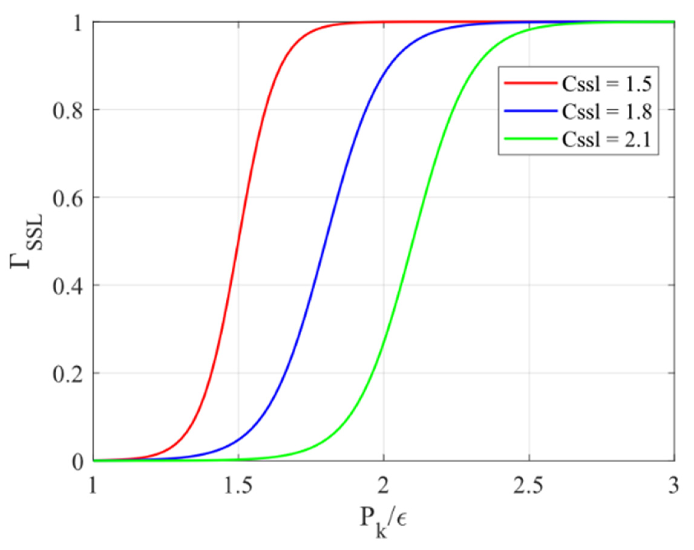
where is the distance between the point considered and the wall. The is larger than one in regions where and , while remains one in other regions. The local value of and decides the magnitude of the modification factor . The diagram of the switch function in Figure 1 illustrates that approaches one when and approaches zero when .
In the fluid region where , approaches zero, and approaches . According to Equation (14), for all values that are physically meaningful, . In the region where , approaches one, and approaches . Equation (14) then indicates that if .
A more physical description is as follows. The modification term is increased in the region away from the wall where the shear presents () and the non-equilibrium turbulence is strong (). The separated shear layer extending from the leading edge of a stalled airfoil has the characteristic mentioned above and is increased there. If is increased, the destruction term in Equation (16) will increase. Therefore, the local value of tends to decrease. The eddy viscosity is approximately proportional to . Therefore, due to the decrease in , the local value of tends to increase. Consequently, the modification term can increase in the separated shear layer. This characteristic makes the SPF model able to avoid the underpredicted in the separated shear layer suffered by many traditional turbulence models [22].
2.3. Numerical Method
All the computations in the following sections are carried out using a finite volume solver (CFL3D version 6.7) [31]. Roe’s flux difference splitting method is used to calculate the inviscid flux at the cell interface:
Here, and are reconstructed by a third-order upwind-biased scheme:
The scalar tridiagonal inversion method is used for matrix inversion [31]. Local time stepping and multigrid are used to accelerate the convergence. The implicit approximate factorization method is used to solve the three transport equations of the SPF model.
The boundary conditions are as follows: the no-slip condition is imposed on the surface of the airfoil, and the free-stream condition is imposed on the outer boundary of the physical domain. For the three transport equations of the SPF model, , and the normal gradient of are set to zero on the no-slip wall boundaries. At the outer boundary of the physical domain, is given, and is computed to match the specified freestream eddy viscosity.
2.4. Grid Convergence Study
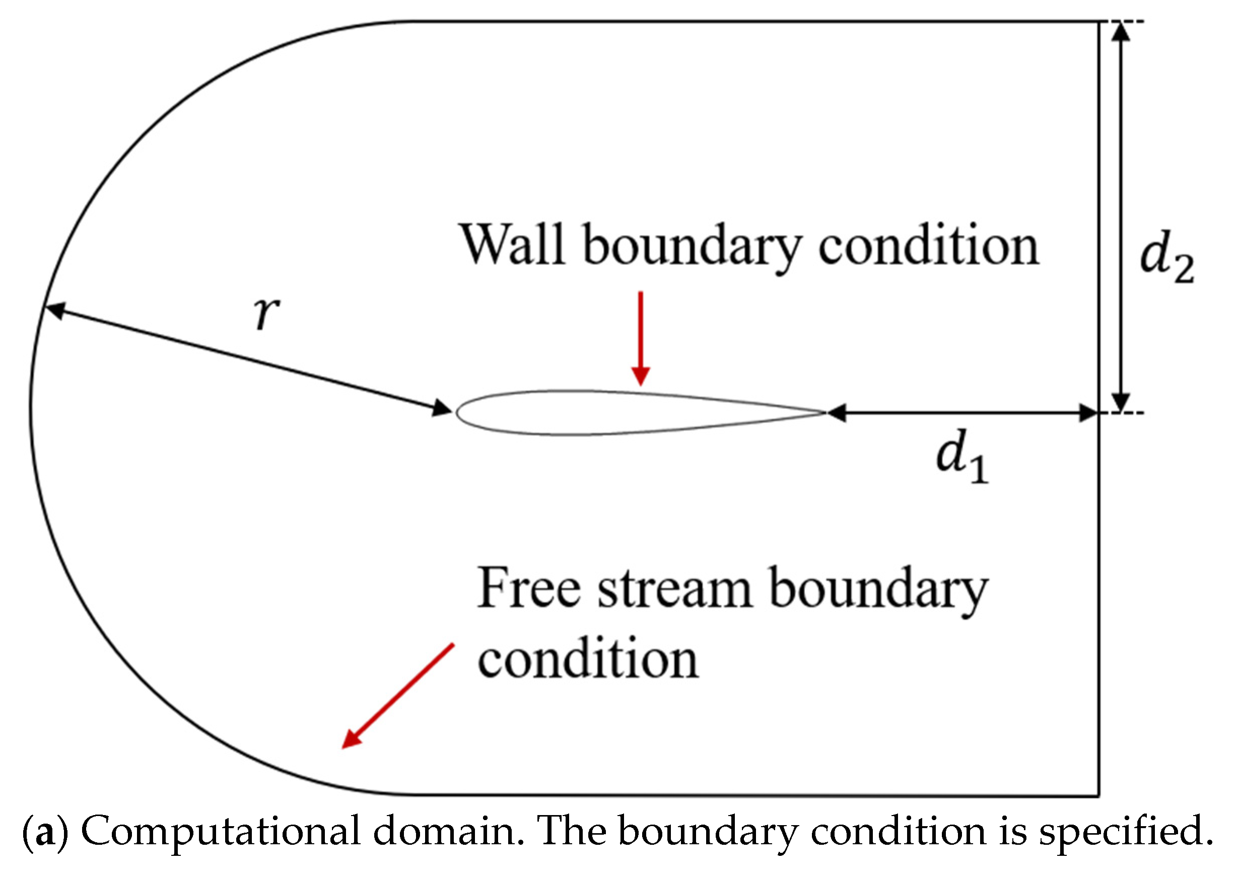
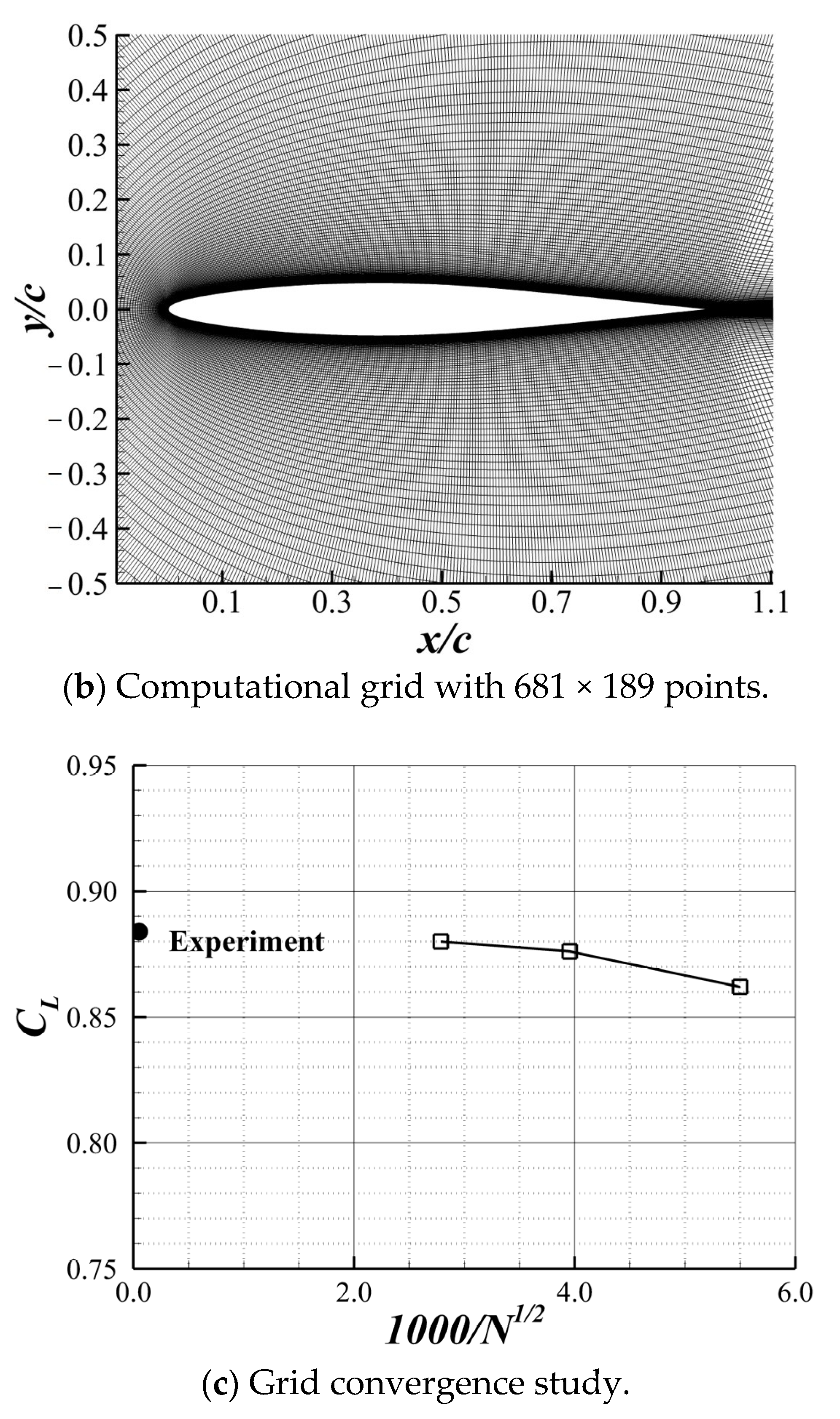
Three C-type grids of the NACA64A010 airfoil with different cell numbers are used for the grid convergence study of the SPF model. The schematic diagram of the computational domain and the boundary conditions are illustrated in Figure 2a. The parameters describe the scales of the computational domain and are equal to 40 times the chord length of the airfoil. The fine grid has 681 and 189 grid points in the circumferential direction and the wall-normal direction, respectively. The medium grid and coarse grid have and grid points, respectively. Figure 2b shows the fine grid used in this paper. The lift coefficients of the NACA64A010 airfoil at , and obtained on these grids are shown in Figure 2c. The lift coefficients are plotted as a function of , where is the number of grid cells. In 2D cases, is proportional to the averaged grid spacing. As shown in Figure 2c, the lift coefficient approached the experimental results [5] as the grid became finer. Consequently, the model exhibited good grid convergent behavior.
3. Numerical Results from Stalled Airfoils
Three test cases are presented in this section. In the first two cases, the SPF model is used to predict the stall characteristics of the NACA64A010 and NACA64A006 airfoils. Both airfoils display thin-airfoil stall. In the third test case, the turbulence model is applied to calculate the aerodynamic performance of the NACA0012 airfoil at large , which undergoes trailing-edge stall at high Reynolds numbers.
3.1. Stall Prediction of the NACA64A010 Airfoil
3.1.1. Low Reynolds Number Case
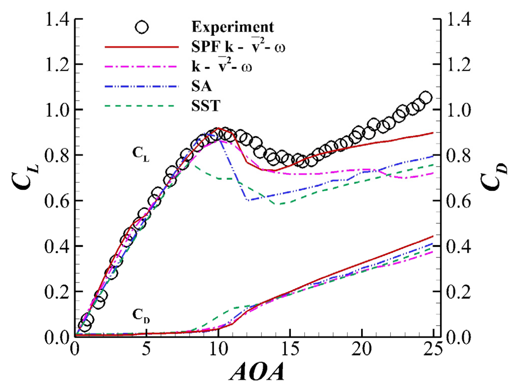
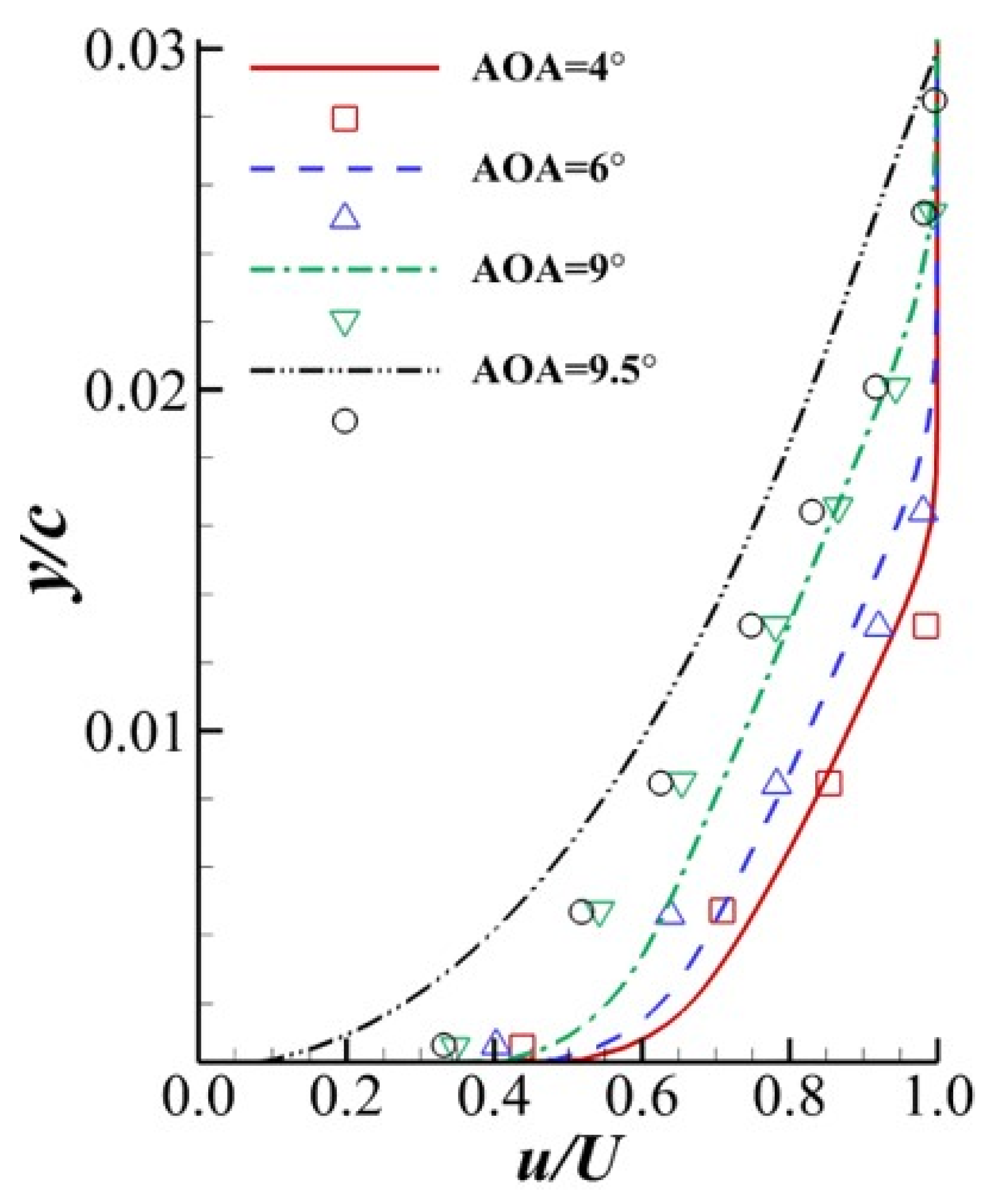
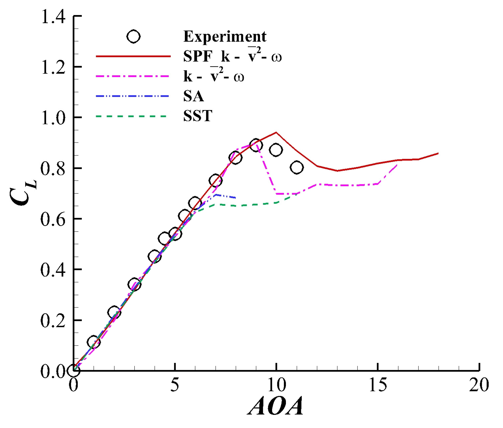
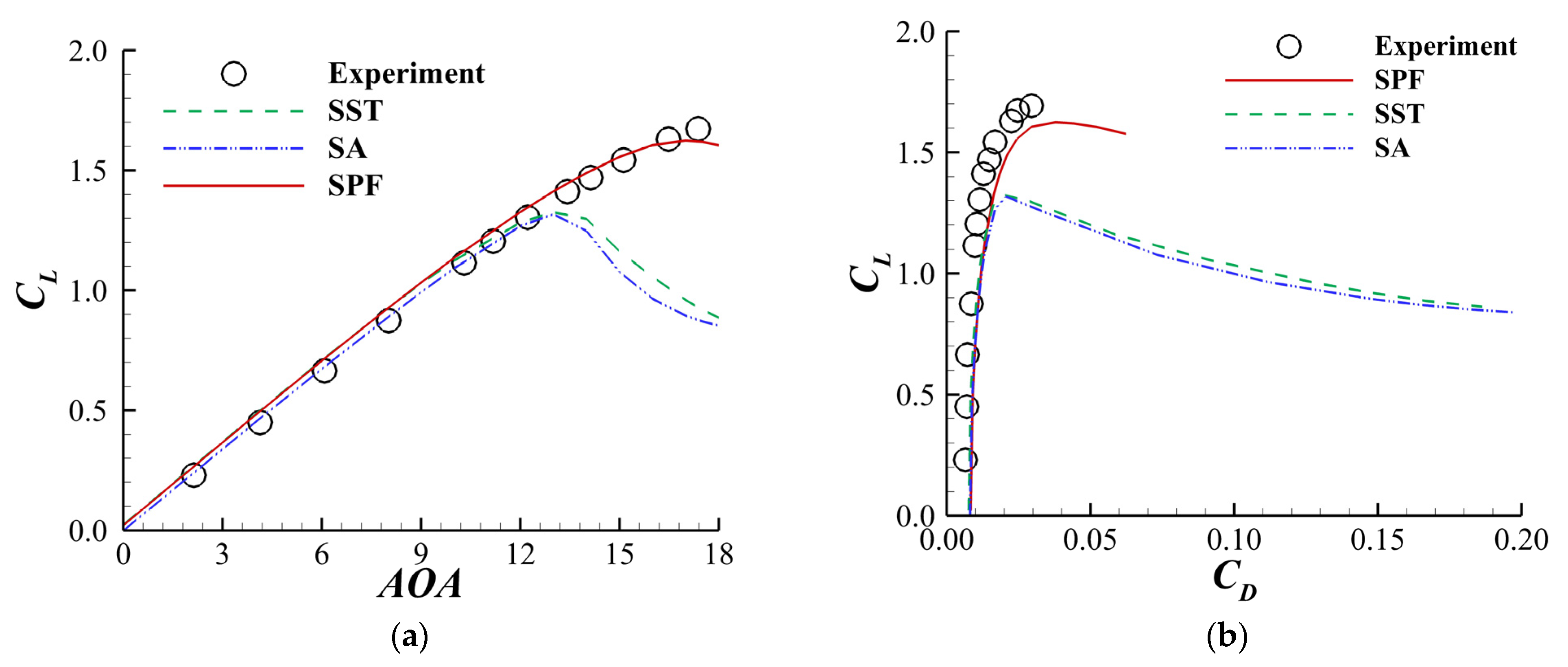
Different turbulence models, including SA [32], SST [33], [20] and SPF (termed the SPF model later in this article), were used to predict the stall behavior of the NACA64A010 airfoil, which underwent thin-airfoil stall. The computation was carried out on the fine grid shown in Figure 2a. The freestream Mach number was 0.12, and the Reynolds number (based on the chord length) was . Figure 3 shows the curves obtained by different turbulence models. The SA and SST models underpredicted at relatively large s. and were also greatly underpredicted by the SST model. The model performed better than the SA and SST models, but the predicted value was still much lower than the experimental value. Unlike the experimental data, the lift curve given by did not rise at . The SPF model predicted and more accurately than the other models, and the curve rose as increased at . Moreover, the relative error between the predicted and experiment was smaller than 3.5%.
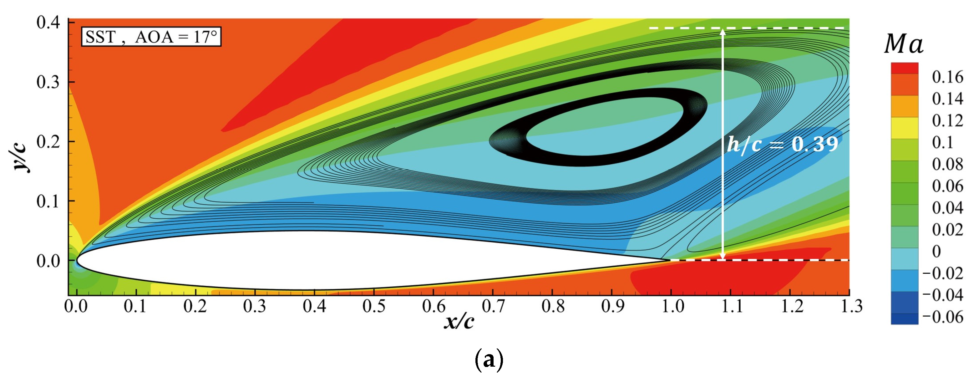
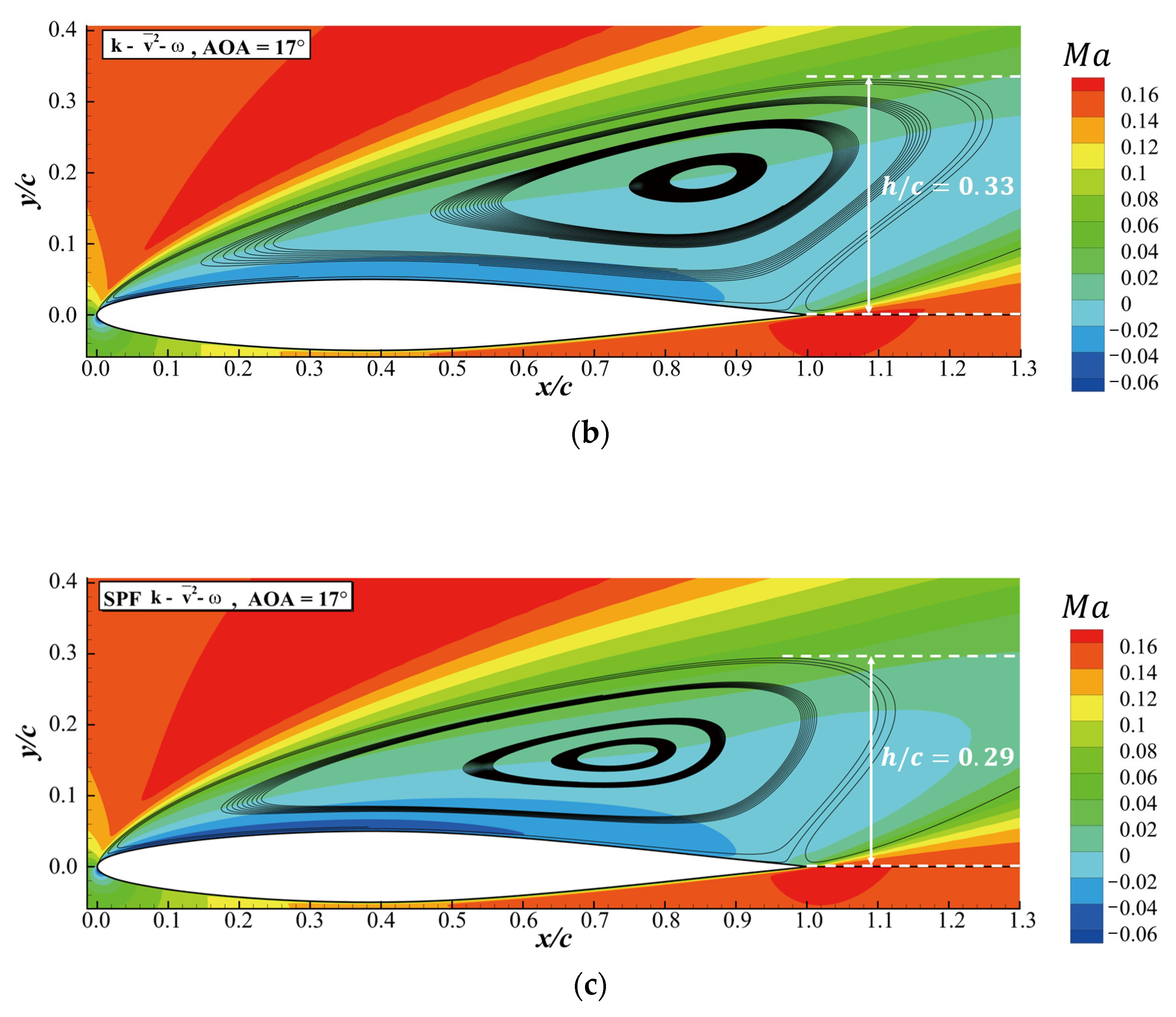
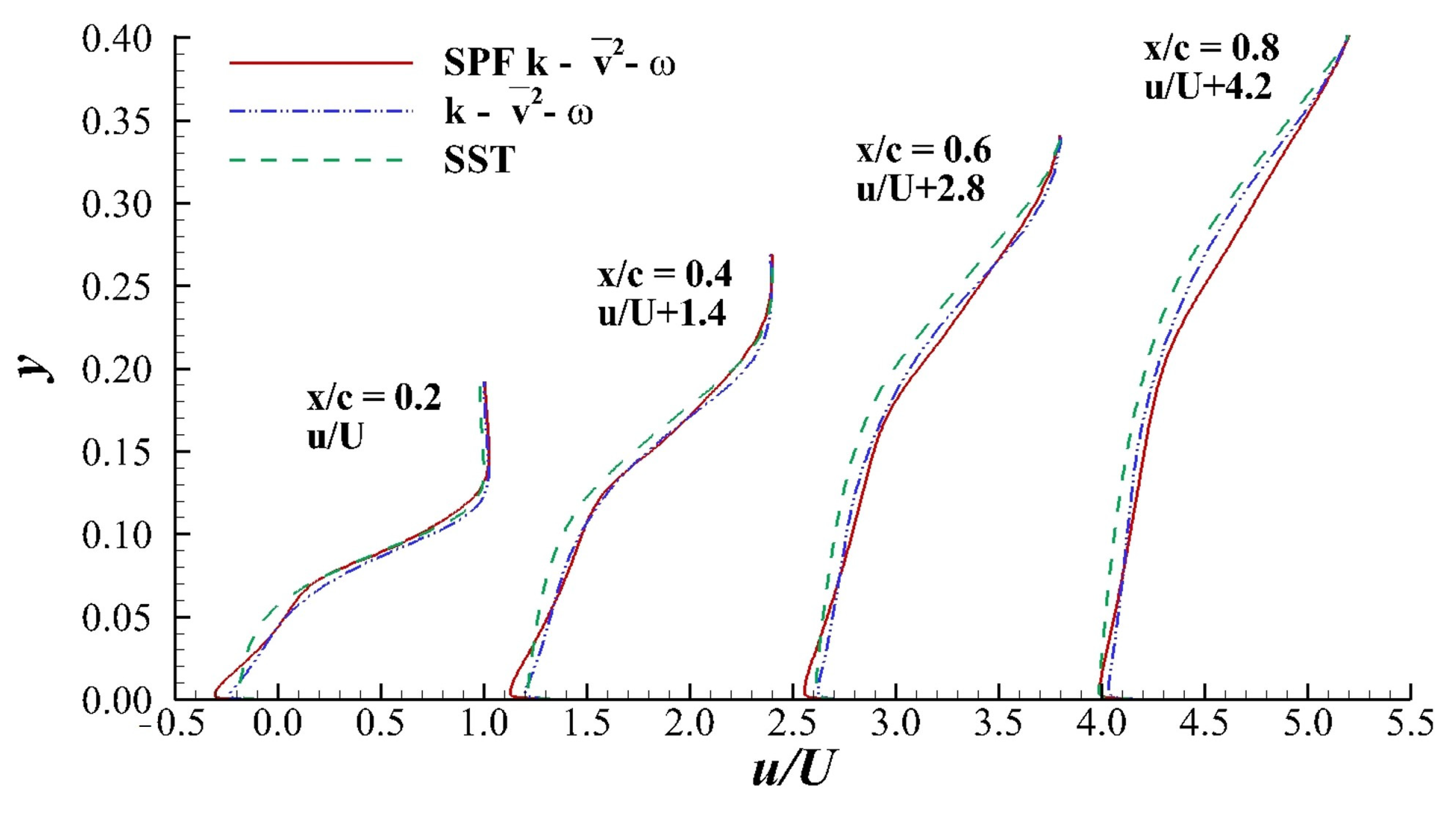
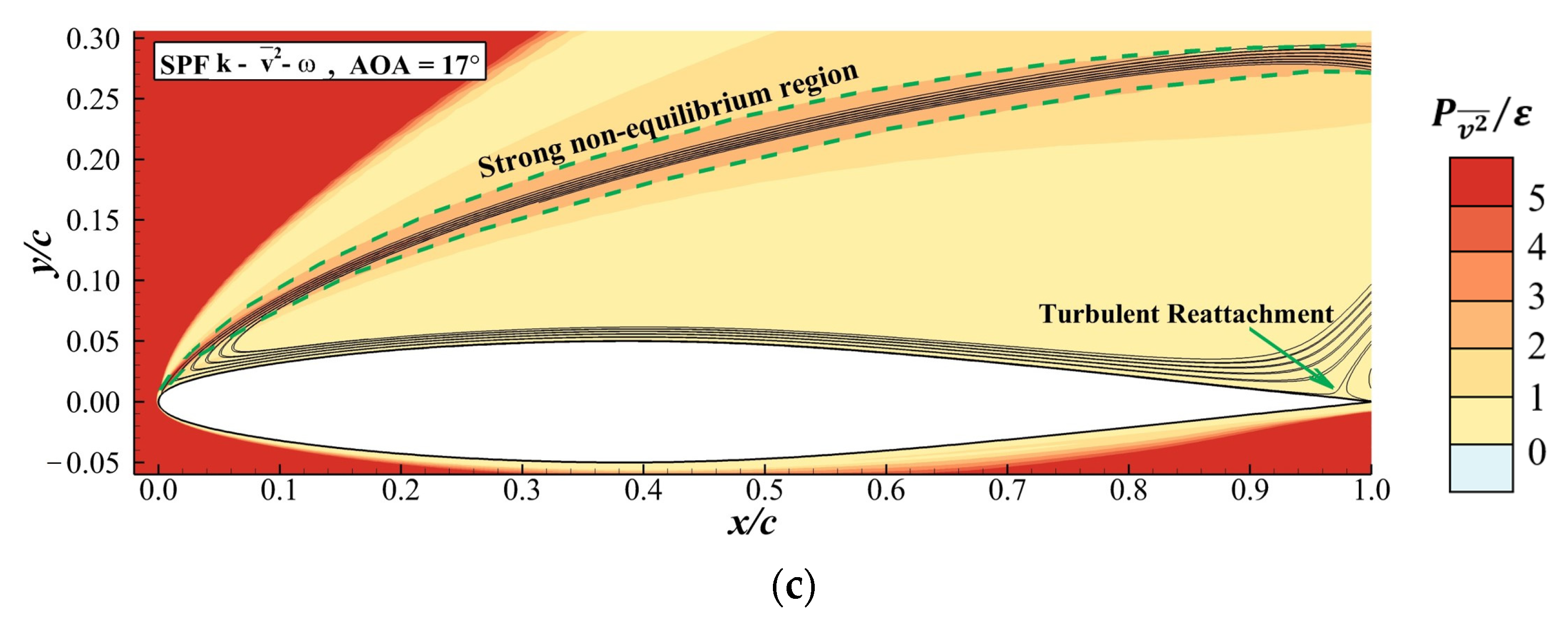
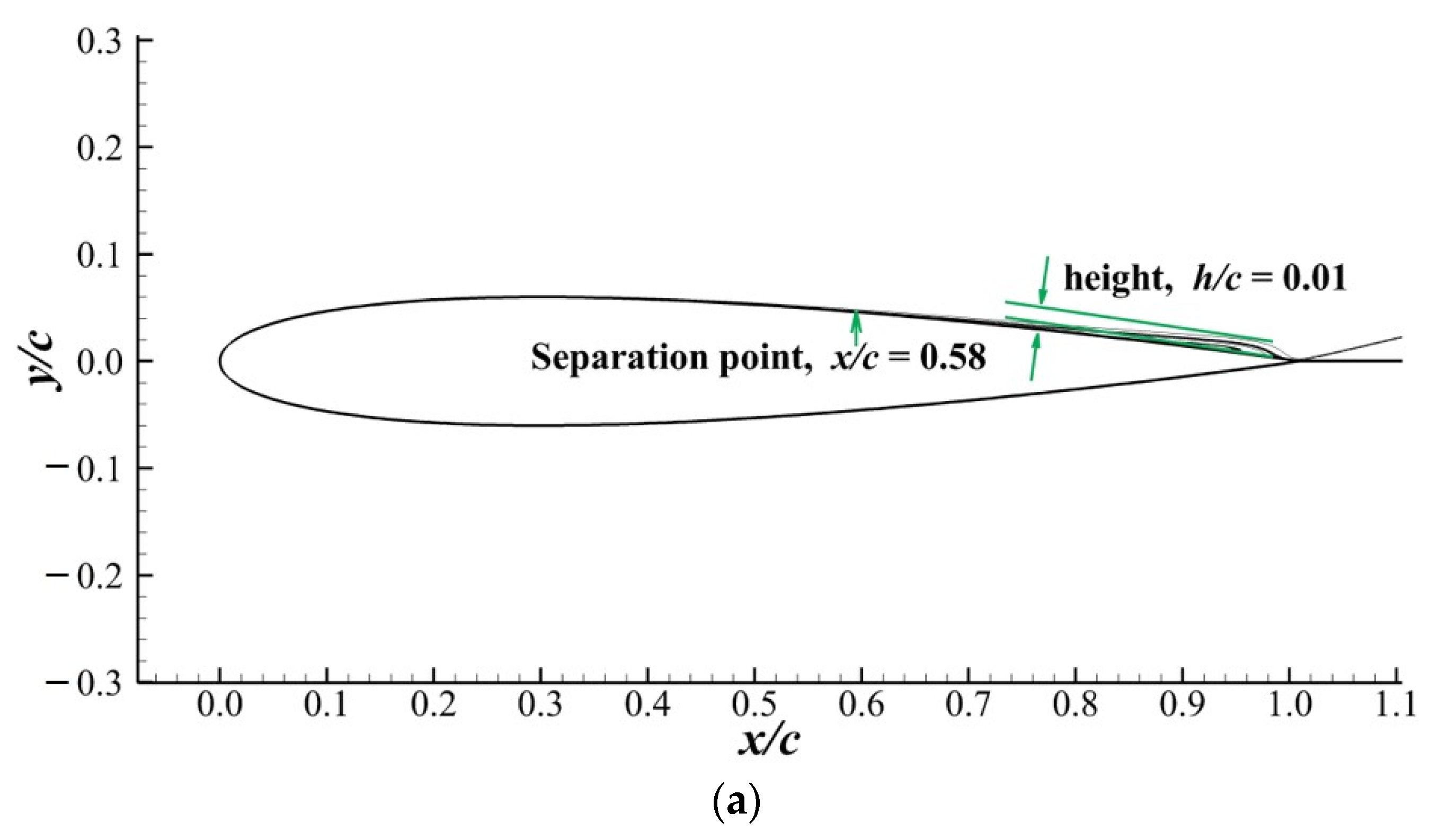
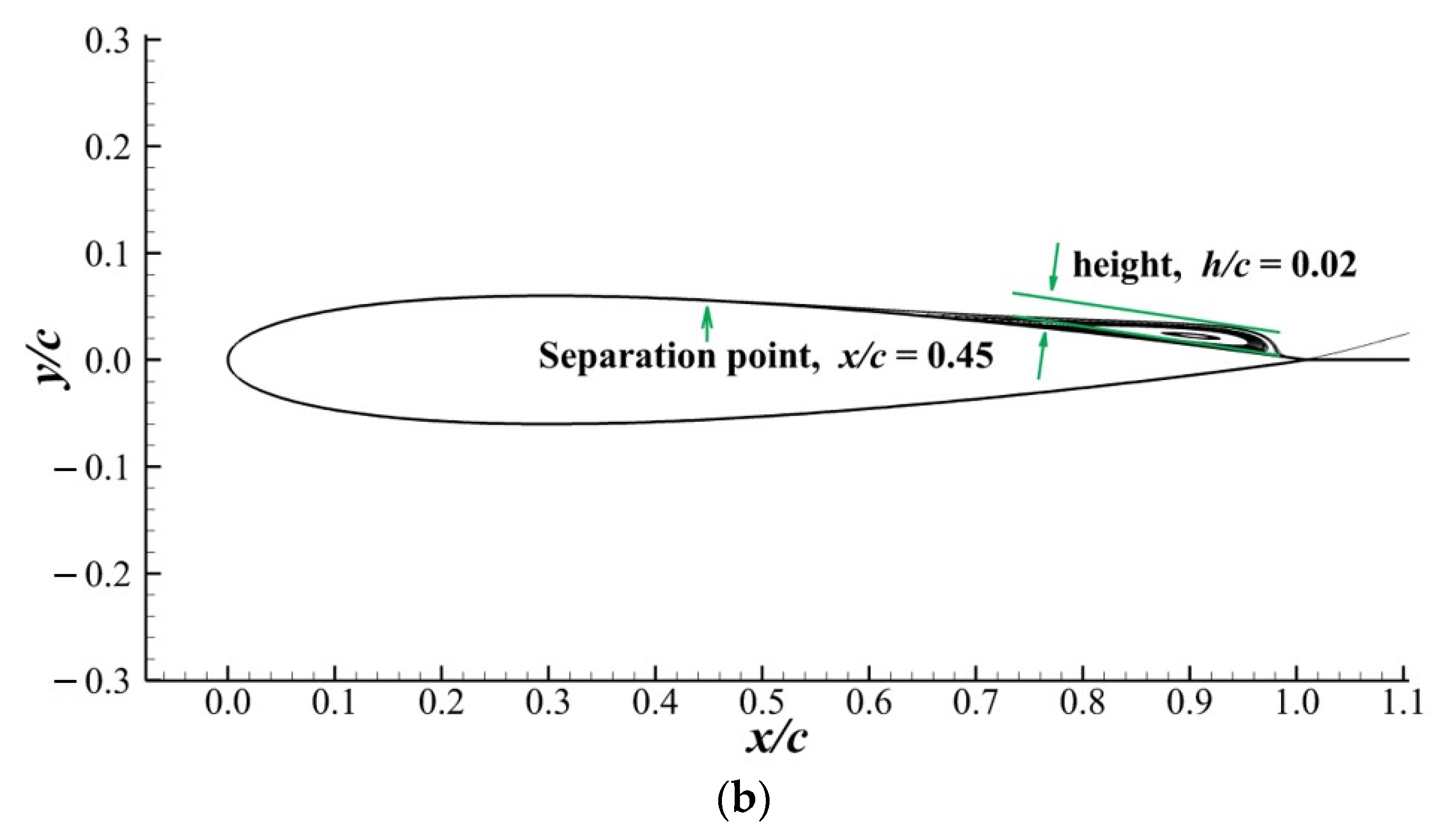
Figure 4 shows the separation bubbles obtained by the SST, and SPF at . The heights of the separation bubbles () given by the SST, and SPF models were 0.39, 0.33 and 0.29, respectively. The SPF model gave the smallest separation bubble. Since the flow with higher momentum encouraged flow reattachment and made the separation bubble shrink, the smaller separation bubble obtained by SPF indicated a flow with greater momentum near the upper surface of the airfoil. The velocity profiles obtained at different stations on the airfoil in Figure 5 confirm that the flow between the airfoil surface and the separated shear layer obtained by the SPF model has a greater velocity compared to the other models. The greater momentum obtained by the SPF model induced a lower pressure coefficient on the upper surface of the airfoil, as shown in Figure 6. The longer interval with lower on the airfoil surface directly led to a larger obtained by the SPF model at , as shown in Figure 3.
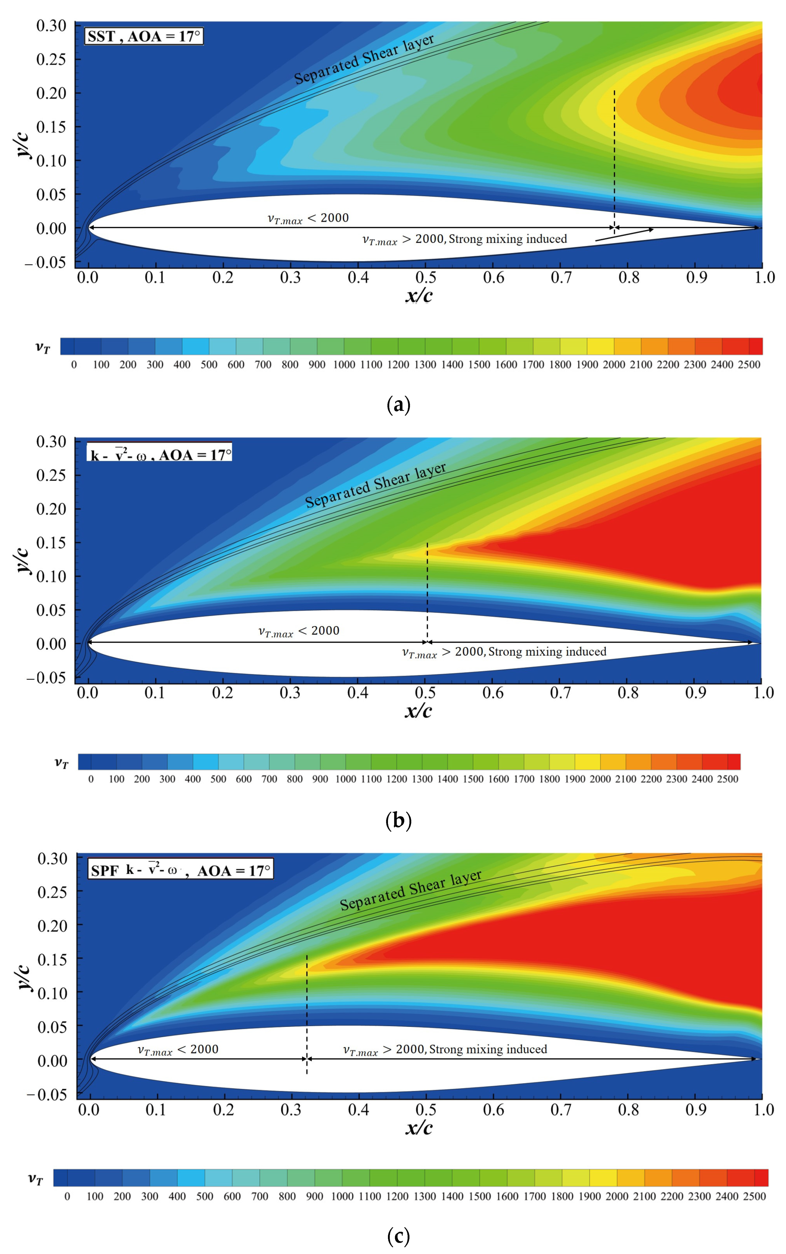
The reason why the SPF model gave a flow with higher momentum between the airfoil surface and the separated shear layer is explained here. In the context of turbulence models based on the Boussinesq hypothesis, a larger can intensify the momentum exchange. Figure 7 shows the contour of given by the SST, and SPF models. The SPF model obtained a larger region where was greater than 2000 compared with the SST and models. Consequently, the momentum exchange was stronger near the separated shear layer in the flow field predicted by the SPF model. Eventually, the stronger momentum exchange will increase the momentum of the flow near the wall. Accordingly, the SPF model gave a shear layer separated from the leading edge, with greater momentum between the separated shear layer and the airfoil surface compared with the SST and models.
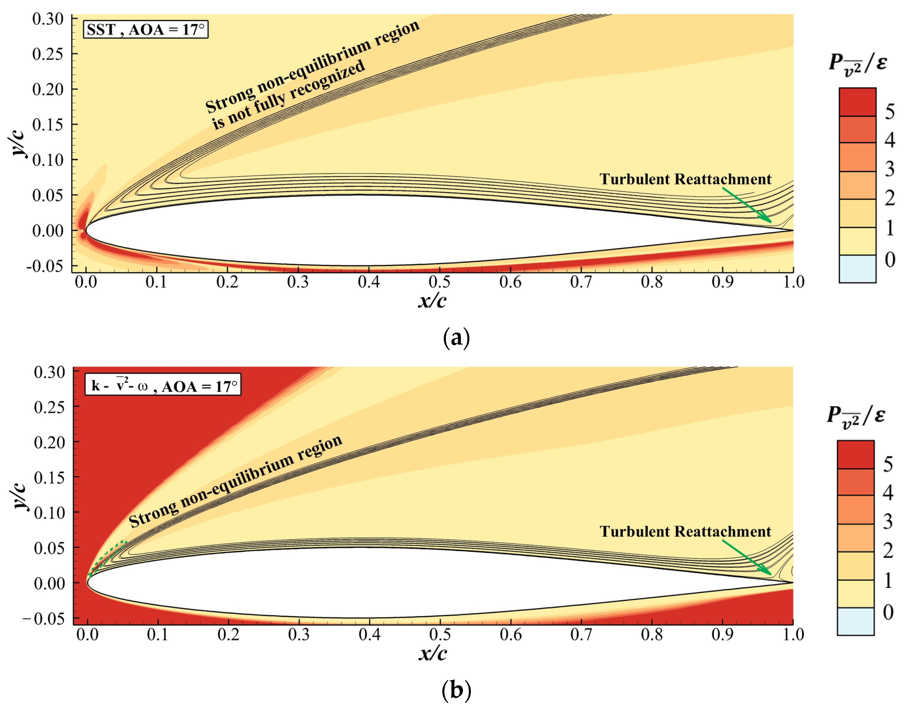
The larger region with a high value obtained by the SPF model was due to the modification introduced to it. Figure 8 shows the contour of at obtained by the SST, and SPF models. Typically, is as high as 3–4 in some part of the separated shear layer [26]. Figure 8a shows that was smaller than two along the separated shear layer, indicating a failure in the prediction of non-equilibrium turbulence. In Figure 8b, predicted a small region in which was greater than two in the separated shear layer. However, this region only extended to . On the other hand, the SPF model predicted that was greater than two along the separated shear layer, as shown in Figure 8c. There was also a region in the separated shear layer that extended to , where was as high as 3–5, which is in agreement with the observation of Rumsey [23]. Consequently, among the three turbulence models considered here, only the SPF model recognized the strong non-equilibrium turbulence in the separated shear layer. The recognition of non-equilibrium turbulence activated the modification in the SPF model through a rapid increase in and then . As shown in Equation (11), the magnified augmented the destruction term of . Since , the decrease in caused by led to an increase in . Finally, a higher induced a lower on the airfoil surface and a larger , as mentioned earlier. Relying on the mechanism discussed above, the SPF model gave a more accurate prediction of at large s.
3.1.2. High Reynolds Number Case
In this section, the NACA64A010 airfoil at the freestream Mach number and the Reynolds number is studied. The computation was carried out on the fine grid shown in Figure 2a. This case was used to test the SPF model’s applicability to thin-airfoil stall problems at high Reynolds numbers. All numerical results were compared with the experiment conducted by Peterson [34]. Figure 9 shows the curves obtained by different turbulence models, including the SA, SST, and SPF models. SA, SST and substantially overpredicted and . The and given by SPF were and 0.98, respectively, and were close to and , which were obtained by the experiment. The relative error between the computed using the SPF model and the experimental result was smaller than 4.0%. On the other hand, the decrease in the lift coefficient after the stall was slightly overpredicted by the SPF model, which led to a more abrupt stall than was observed in the experiment. However, the result given by the SPF model obviously showed the best agreement with the experimental data among the four turbulence models.
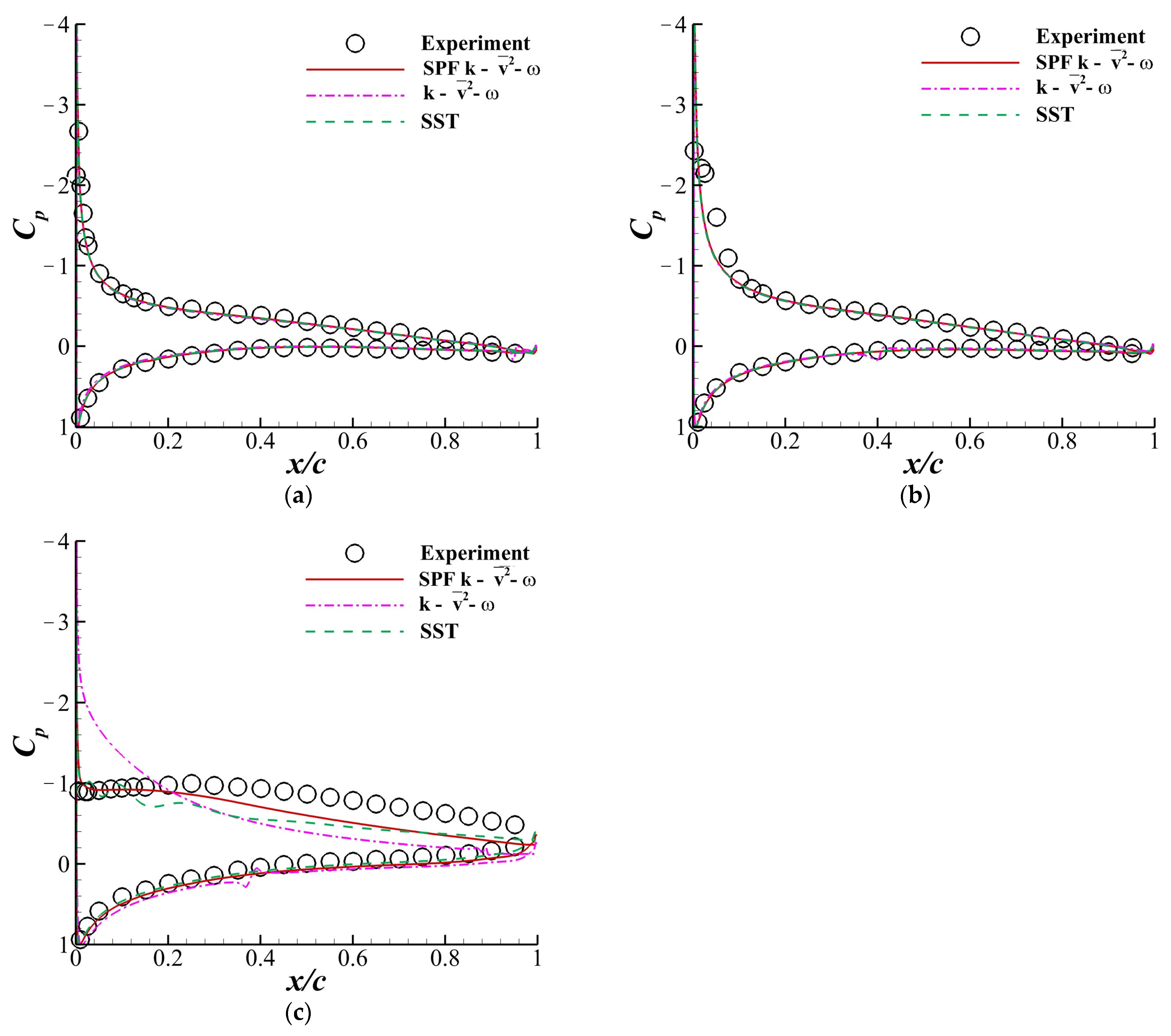
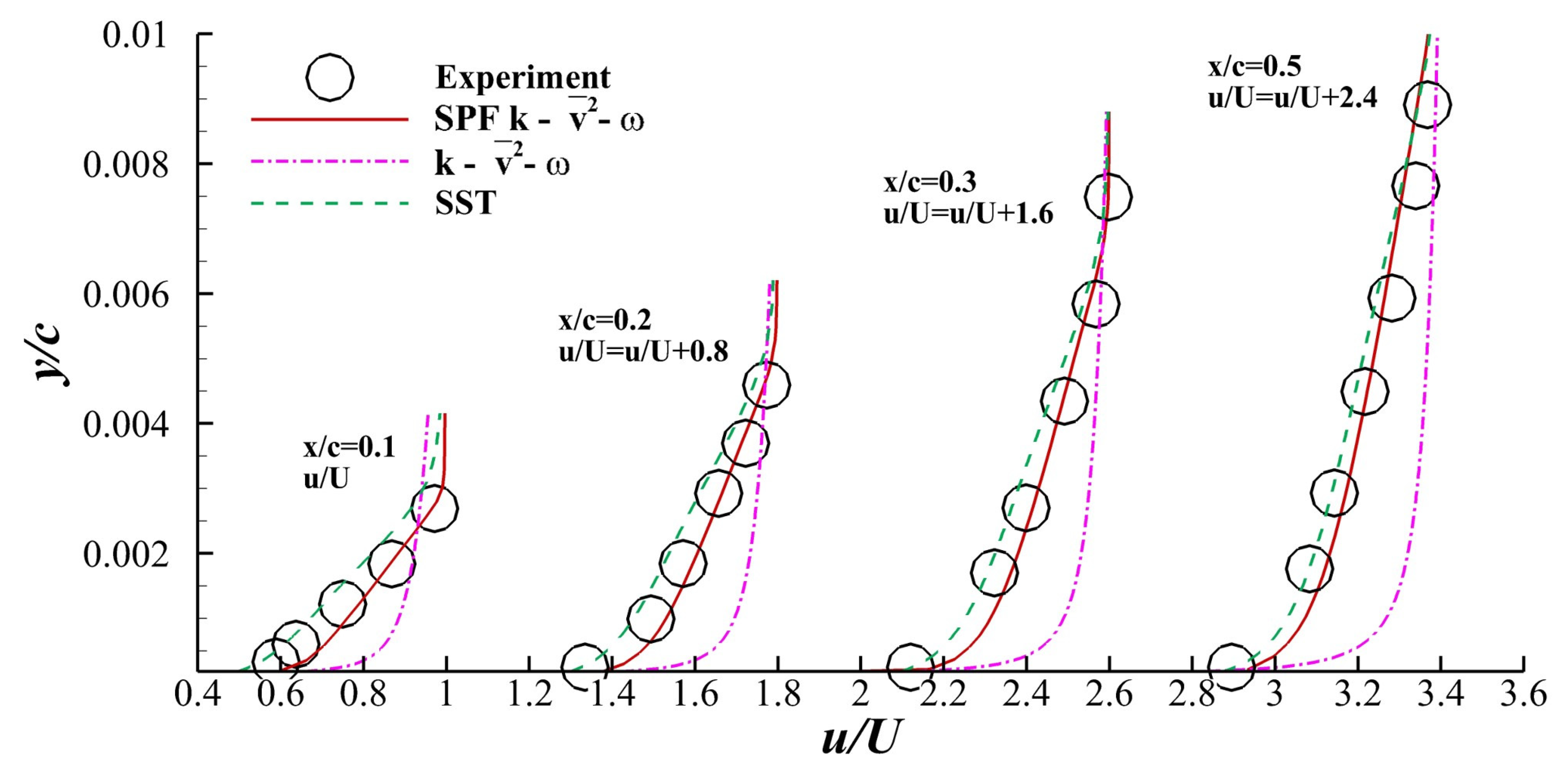
Figure 10 shows the pressure distributions on the airfoil at and . The results obtained by SPF, SST and SA agreed well with the experimental results. The model gave the pressure distribution with a zigzag pattern, which showed poor convergence in the steady RANS computation. Figure 11 shows the velocity profiles at obtained by the SPF model. The scatter diagram represents the experimental data, and the curves represent the results obtained by the SPF model. The computational results agreed well with the experiment at , and . However, the velocity profile obtained by the SPF model was slightly different from the experiment at . This difference corresponded to the sharp stall in Figure 9 calculated by the SPF model. In conclusion, the SPF model performed better than the SST, SA and models at predicting the stall characteristics of the NACA64A010 airfoil at high Reynolds numbers.
3.2. Stall Prediction of the NACA64A006 Airfoil
The SPF model was used to predict the stalling behavior of the NACA64A006 airfoil, which exhibited thin-airfoil stalling characteristics. The experimental results obtained by McCullough et al. [35] were used to test the accuracy of the numerical results. The freestream Mach number was , and the Reynolds number (based on the chord length) was . A C-type grid like Figure 2a was adopted. This case was chosen to test whether the fixed SPF model had general applicability in thin-airfoil stall problems.
Figure 12 shows the curves obtained by different turbulence models, including SA, SST, and SPF. and were both seriously underpredicted by SA and SST. The computation using these two models quickly diverged after . The model performed relatively better. However, the curve jumped after , and the computation diverged at . The SPF model still obtained the result closest to the experiment among all four turbulence models. For the SPF model, the relative error between the computed and the experimental result was smaller than 5.5%. The lift coefficient predicted by the SPF model rose as increased at large , which is a typical characteristic of a thin-airfoil stall.
Figure 13 shows the distributions on the airfoil surface obtained by the SPF, , SST and experimental data. All numerical results agreed well with the experiment at and . At , the model failed to predict a flat distribution on the upper surface, while the SST model gave a wavy distribution that was not observed in the experiment. The SPF model successfully captured the flat distribution, and the result agreed well with the experiment. Figure 14 shows the velocity profiles in the boundary layer at given by the SPF, and SST models and the experiment. The figure illustrates that at all stations selected, the prediction of the velocity profile given by the SPF model agreed well with the experiment, while overestimated the velocity and SST underestimated the velocity at most locations. The accurate computation of the boundary layer velocity profile constituted a basis for the SPF model to correctly predict the flow separation associated with the airfoil stall. Considering the relatively precise prediction of and the details of the flow field, the fix in the SPF model had some general applicability in the prediction of the thin-airfoil stall.
3.3. Stall Prediction of the NACA0012 Airfoil
The stall characteristics of the NACA0012 airfoil are reported in this section. The freestream Mach number was , and the Reynolds number (based on the chord length) was . All the numerical results were compared with the experiment carried out by Ladson [36]. The computation was carried out on a C-type grid that had grid points in the circumferential direction and grid points in the normal direction.
According to Gregory and Reilly [37], the NACA0012 airfoil only exhibits trailing-edge stalling characteristics at the Reynolds number . The boundary layer separation point moves from the trailing edge to the leading edge, and the separation bubble grows in size as increases before the airfoil stall. The separation point is not fixed while the non-equilibrium turbulence is not that strong in the separated shear layer. Consequently, the flow pattern in this case differs from the previous patterns, except that the separated shear layer still presents itself.
Figure 15a,b shows the curve and drag polar curves obtained by the SST, SA and SPF models. The result of the model is not presented here because the computation had difficulty converging at this case. The SST and SA models seriously underestimated and , while the SPF model underestimated them by only and 0.06, respectively. The relative error between the computed and the experimental data was smaller than 3.5% when the experimental . Because of underestimated , both the SST and SA models gave drag polar curves that dramatically deviated from the experiment. On the other hand, the drag polar curve obtained by SPF started to deviate from the experiment only at a larger . Therefore, the SPF model predicted the force coefficient near the stall more accurately than the other two models.
Figure 16a,b shows the streamlines past the airfoil at and obtained by the SPF model. At both angles of attack, there was a separation bubble near the trailing edge. As the angle of attack increased from to , the separation point moved forward, and the separation bubble grew, which is exactly the characteristic of trailing-edge stall. This indicates that the SPF model correctly captured the features of boundary layer separation in the trailing-edge stall. Consequently, the SPF model’s applicability was not limited to thin-airfoil stall problems. The model for trailing-edge stall prediction was also satisfactory.
4. Conclusions
Stall is a typical flow phenomenon for an airfoil operating at large angles of attack. To accurately predict airfoil stall, an accurate RANS model is expected to reflect the non-equilibrium characteristic of turbulence in the separated shear layer. In this paper, the SA, SST, and SPF models were used to compute the stall performance of the NACA64A010, NA64A006 and NACA0012 airfoils. The SA and SST models were mainly calibrated for equilibrium turbulence, and these models failed to predict the airfoil stall performance. The SPF model supplemented by the separated shear layer fix terms captured the non-equilibrium characteristic in the shear layers successfully and predicted the stall performance accurately. The work of this paper can be summarized as follows:
(1) The SPF model was proven to be effective for the stall prediction of NACA64A006 and NACA64A010 airfoils at different Reynolds numbers, which all feature thin-airfoil stall. The relative errors between the computed and the experimental data at both cases were less than 5.5%.
(2) The SPF model was also applied to predict the stall of the NACA0012 airfoil, which exhibited a trailing-edge stalling feature. The relative error between the predicted and the experimental data was smaller than 3.5% when the lift . The SPF model also showed good effectiveness on the trailing-edge stall problem.
The authors believe that the SPF model can also be applied to other airfoils featuring thin-airfoil stall and trailing-edge stall if the subsonic flow is considered. Hence, the SPF model has the potential to be applied to the verification of the stall performance and the numerical optimization of an airfoil’s stall performance.
We need to further explore the applicability of the model in the 3D cases and the 3D corrections that may be needed. This is because the stall performance of a 3D wing is also critical in aircraft design. In addition, we need to consider turbulence models that take fluid compressibility into account and are capable of stall prediction, given that many current aircraft are faster and may continue to get faster.
Author Contributions
Conceptualization, C.W., H.L., and Y.Z.; methodology, C.W., H.L.; software, H.L.; validation, H.L.; formal analysis, C.W., and H.L.; investigation, C.W. and H.L.; resources, Y.Z. and H.C.; data curation, C.W. and H.L.; writing—original draft preparation, C.W.; writing—review and editing, C.W., Y.Z. and H.L.; visualization, C.W. All authors have read and agreed to the published version of the manuscript.
Funding
This research received no external funding.
Data Availability Statement
The data presented in this study are available on request from the corresponding author. The data are not publicly available due to the large volume of data.
Acknowledgments
This work was supported by the National Natural Science Foundation of China under grant Nos. 11872230, 91852108, 92052203 and 91952302.
Conflicts of Interest
The authors declare no conflict of interest.
Nomenclature
| angle of attack (deg) | |
| stall angle of attack (deg) | |
| lift coefficient | |
| maximum lift coefficient | |
| pressure coefficient | |
| airfoil chord length (m) | |
| Reynolds number | |
| fluid velocity (m/s) | |
| magnitude of vorticity (1/s) | |
| density (kg/m3) | |
| pressure (kg·m/s2) | |
| kinematic molecular viscosity (m2/s) | |
| production rate of turbulent kinetic energy (m2/s3) | |
| dissipation rate of turbulent kinetic energy (m2/s3) |
Appendix A. The SPF Model
Appendix A.1. Definition of the Terms
The transport equations of the SPF model are
The production terms in the transport equations can be expressed as
in Equation (A4) can be calculated from the velocity field:
The turbulence viscosity can be calculated by
, and the damping function can be expressed as
can be written as
The intermittency damping function and the parameter can be written as
is defined as
The last two terms we need to calculate the eddy viscosity in Equation (A6) can be expressed as
The dissipation terms of Equations (A1) and (A2) can be written as
The effective diffusivity in the diffusion term of Equations (A1) and (A2) is
The blending function in the fourth term at the right-hand side of Equation (A3) is expressed as
is expressed as
represents the natural transition effect and is expressed as
is defined as
represents the effect of the bypass transition and is defined as
The definition of the modification term in the destruction term of ’s transport equation can be found in Section 2.2.
Appendix A.2. The Value of the Constants
According to the calibration carried out by Lopez et al. [20] and Li et al. [27], the value of the constants in the model are listed below:

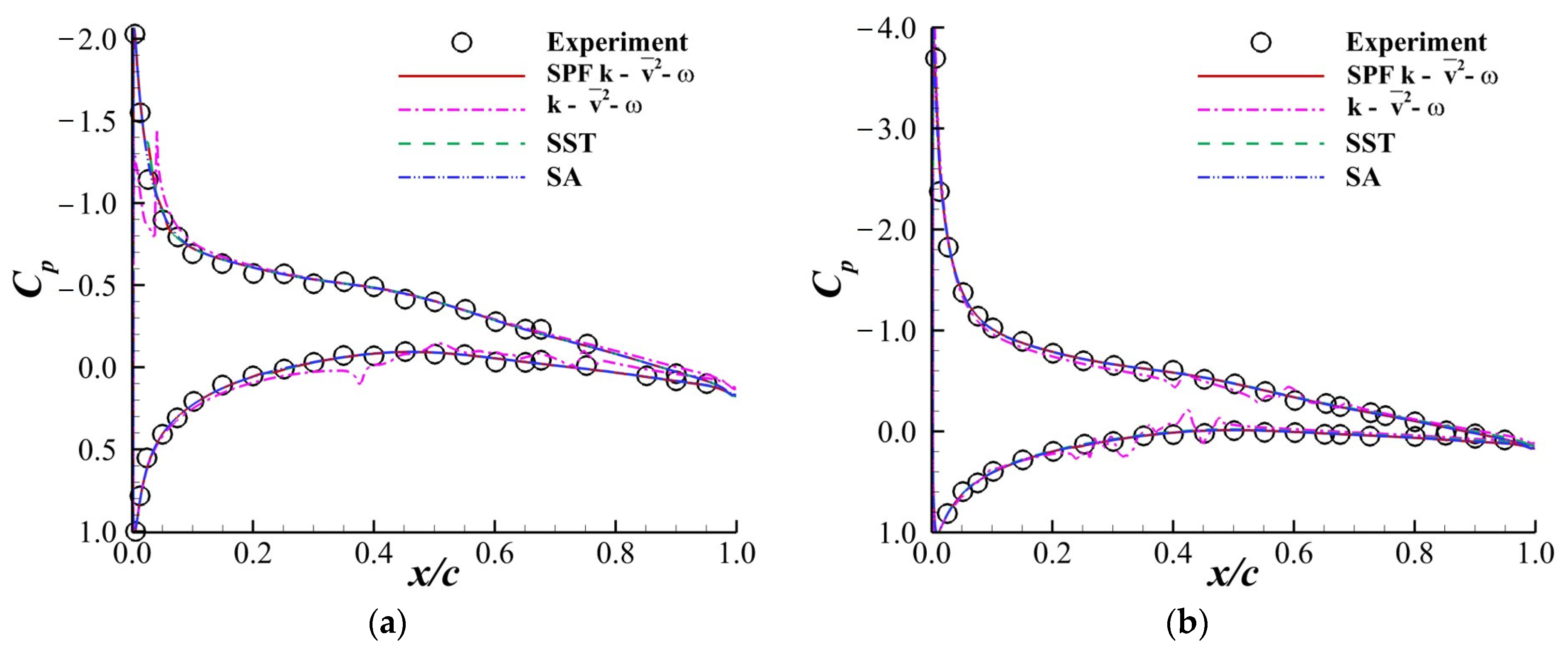
Table A1.
The value of the parameters in the SPF Model.
References
- Broeren, A.P. An Experimental Study of Unsteady Flow over Airfoils Near Stall; University of Illinois at Urbana-Champaign: Champaign, IL, USA, 2000. [Google Scholar]
- Vu, N.; Lee, J. Aerodynamic design optimization of helicopter rotor blades including airfoil shape for forward flight. Aerosp. Sci. Technol. 2015, 42, 106–117. [Google Scholar] [CrossRef]
- Fusi, F.; Congedo, P.M.; Guardone, A.; Quaranta, G. Assessment of robust optimization for de-sign of rotorcraft airfoils in forward flight. Aerosp. Sci. Technol. 2020, 107, 106355. [Google Scholar] [CrossRef]
- McCullough, G.B.; Gault, D.E. Examples of Three Representative Types of Airfoil-Section Stall at Low Speed; National Advisory Committee for Aeronautics: Kitty Hawk, NC, USA, 1951. [Google Scholar]
- Broeren, A.P.; Bragg, M.B. Spanwise Variation in the Unsteady Stalling Flowfields of Two-Dimensional Airfoil Models. AIAA J. 2001, 39, 1641–1651. [Google Scholar] [CrossRef]
- Tani, I. Low-speed flows involving bubble separations. Prog. Aerosp. Sci. 1964, 5, 70–103. [Google Scholar] [CrossRef]
- Gleyzes, C.; Capbern, P. Experimental study of two AIRBUS/ONERA airfoils in near stall conditions. Part I: Boundary layers. Aerosp. Sci. Technol. 2003, 7, 439–449. [Google Scholar] [CrossRef]
- Rodríguez, I.; Lehmkuhl, O.; Borrell, R.; Oliva, A. Direct numerical simulation of a NACA0012 in full stall. Int. J. Heat Fluid Flow 2013, 43, 194–203. [Google Scholar] [CrossRef] [Green Version]
- Mary, I.; Sagaut, P. Large eddy simulation of flow around an airfoil near stall. AIAA J. 2002, 40, 1139–1145. [Google Scholar] [CrossRef]
- Im, H.-S.; Zha, G.-C. Delayed Detached Eddy Simulation of Airfoil Stall Flows Using High-Order Schemes. J. Fluids Eng. 2014, 136, 111104. [Google Scholar] [CrossRef]
- Kawai, S.; Fujii, K. Prediction of a thin-airfoil stall phenomenon using LES/RANS hybrid methodology with compact difference scheme. In Proceedings of the 34th AIAA Fluid Dynamics Conference and Exhibit, Portland, OR, USA, 28 June–1 July 2004; p. 2714. [Google Scholar]
- Menter, F.R.; Kuntz, M.; Langtry, R. Ten years of industrial experience with the SST turbulence model. Turbul. Heat Mass Transf. 2003, 4, 625–632. [Google Scholar]
- Allmaras, S.R.; Johnson, F.T. Modifications and clarifications for the implementation of the Spalart-Allmaras turbulence model. In Proceedings of the Seventh International Conference on Computational Fluid Dynamics (ICCFD7), Big Island, HI, USA, 9–13 July 2012; Volume 1902. [Google Scholar]
- Rizzetta, D.P.; Visbal, M.R.; Visbalt, M.R. Comparative Numerical Study of Two Turbulence Models for Airfoil Static and Dynamic Stall. AIAA J. 1993, 31, 784–786. [Google Scholar] [CrossRef]
- Genç, M. Numerical simulation of flow over a thin aerofoil at a high Reynolds number using a transition model. Proc. Inst. Mech. Eng. Part C J. Mech. Eng. Sci. 2010, 224, 2155–2164. [Google Scholar] [CrossRef]
- Catalano, P.; Tognaccini, R. RANS analysis of the low-Reynolds number flow around the SD7003 airfoil. Aerosp. Sci. Technol. 2011, 15, 615–626. [Google Scholar] [CrossRef]
- Wokoeck, R.; Krimmelbein, N.; Ortmanns, J.; Ciobaca, V.; Radespiel, R.; Krumbein, A. RANS Simulation and Experiments on the Stall Behaviour of an Airfoil with Laminar Separation Bubbles. In Proceedings of the 44th AIAA Aerospace Sciences Meeting and Exhibit, Reno, Nevada, 9–12 January 2006. [Google Scholar] [CrossRef]
- Walters, D.K.; Leylek, J.H. Computational Fluid Dynamics Study of Wake-Induced Transition on a Compressor-Like Flat Plate. J. Turbomach. 2005, 127, 52–63. [Google Scholar] [CrossRef]
- Mayle, R.E.; Schulz, A. Heat Transfer Committee and Turbomachinery Committee Best Paper of 1996 Award: The Path to Predicting Bypass Transition. J. Turbomach. 1997, 119, 405–411. [Google Scholar] [CrossRef]
- Lopez, M.; Walters, D.K. Prediction of transitional and fully turbulent flow using an alternative to the laminar kinetic energy approach. J. Turbul. 2016, 17, 253–273. [Google Scholar] [CrossRef]
- Morgado, J.; Vizinho, R.; Silvestre, M.; Páscoa, J. XFOIL vs. CFD performance predictions for high lift low Reynolds number airfoils. Aerosp. Sci. Technol. 2016, 52, 207–214. [Google Scholar] [CrossRef]
- Rumsey, C. Successes and Challenges for Flow Control Simulations. Int. J. Flow Control. 2008, 1, 4311. [Google Scholar] [CrossRef] [Green Version]
- Rumsey, C.L.; Gatski, T.; Sellers III, W.; Vasta, V.; Viken, S. Summary of the 2004 computation-al fluid dynamics validation workshop on synthetic jets. AIAA J. 2006, 44, 194–207. [Google Scholar] [CrossRef]
- Fang, L.; Zhao, H.; Ni, W.; Fang, J.; Lu, L. Non-equilibrium turbulent phenomena in the flow over a backward-facing ramp. Appl. Math. Mech. 2019, 40, 215–236. [Google Scholar] [CrossRef]
- Fang, L.; Zhao, H.-K.; Lu, L.-P.; Liu, Y.; Yan, H. Quantitative description of non-equilibrium turbulent phenomena in compressors. Aerosp. Sci. Technol. 2017, 71, 78–89. [Google Scholar] [CrossRef]
- Rumsey, C.L. Exploring a Method for Improving Turbulent Separated-Flow Predictions with Kappa-Omega Models; NASA: Washington, DC, USA, 2009. [Google Scholar]
- Li, H.; Zhang, Y.; Chen, H. Aerodynamic Prediction of Iced Airfoils Based on Modified Three-Equation Turbulence Model. AIAA J. 2020, 58, 3863–3876. [Google Scholar] [CrossRef]
- Li, H.; Zhang, Y.; Chen, H. Optimization of supercritical airfoil considering the ice-accretion effects. AIAA J. 2019, 57, 4650–4669. [Google Scholar] [CrossRef]
- Li, H.; Zhang, Y.; Chen, H. Numerical Simulation of Iced Wing Using Separating Shear Layer Fixed Turbulence Models. AIAA J. 2021, 59, 3667–3681. [Google Scholar] [CrossRef]
- Zhang, S.; Li, H.; Zhang, Y.; Chen, H. Aerodynamic Prediction of High-Lift Configuration Using k-(v^2 )-ω Turbulence Model. AIAA J. arXiv 2021, arXiv:2105.12521. [Google Scholar] [CrossRef]
- Rumsey, C. “CFL3D Version 6 Home Page” NASA. 1980. Available online: https://cfl3d.larc.nasa.gov/ (accessed on 1 October 2019).
- Spalart, P.; Allmaras, S. A one-equation turbulence model for aerodynamic flows. Rech. Aerosp. 1994, 1, 5–21. [Google Scholar]
- Menter, F.R. Two-equation eddy-viscosity turbulence models for engineering applications. AIAA J. 1994, 32, 1598–1605. [Google Scholar] [CrossRef] [Green Version]
- Peterson, R.F. The Boundary-Layer and Stalling Characteristics of the NACA 64A010 Airfoil Section; National Advisory Committee for Aeronautics: Kitty Hawk, NC, USA, 1950. [Google Scholar]
- McCullough, G.B.; Gault, D.E. Boundary-Layer and Stalling Characteristics of the NACA 64A006 Airfoil Section; National Advisory Committee for Aeronautics: Kitty Hawk, NC, USA, 1949. [Google Scholar]
- Ladson, C.L. Effects of Independent Variation of Mach and Reynolds Numbers on the Low-Speed Aero-Dynamic Characteristics of the NACA 0012 Airfoil Section; National Aeronautics and Space Administration, Scientific and Technical: Kitty Hawk, NC, USA, 1988. [Google Scholar]
- Gregory, N.; O’reilly, C. Low-Speed Aerodynamic Characteristics of NACA 0012 Aerofoil Section, Including the Effects of Upper-Surface Roughness Simulating Hoar Frost; National Advisory Committee for Aeronautics: Kitty Hawk, NC, USA, 1970. [Google Scholar]
Figure 1.
The diagram of when the parameter is 1.5, 1.8 and 2.1.

Figure 2.
(a) The schematic diagram of the computational domain with boundary conditions, where is the radius of the outer boundary in front of the airfoil, is the distance between the trailing edge of the airfoil and the left boundary and is the half width of the computational domain. (b) Fine grid of NACA64A010. (c) Grid convergence study at and .


Figure 3.
curve obtained by different turbulence models of the NACA64A010 airfoil when and . The circles represent experimental data obtained by Broeren et al. [5].
Figure 3.
curve obtained by different turbulence models of the NACA64A010 airfoil when and . The circles represent experimental data obtained by Broeren et al. [5].

Figure 4.
Separation bubble at and on the NACA64A010 airfoil. The relative height of the separation bubble is marked in the figures. (a) SST model. (b) model. (c) SPF model.
Figure 4.
Separation bubble at and on the NACA64A010 airfoil. The relative height of the separation bubble is marked in the figures. (a) SST model. (b) model. (c) SPF model.


Figure 5.
Velocity profiles given by SST, and SPF models on the upper surface of the airfoil at , , and . and . The profiles are shifted for clarity.
Figure 5.
Velocity profiles given by SST, and SPF models on the upper surface of the airfoil at , , and . and . The profiles are shifted for clarity.

Figure 6.
distributions on the surface of the airfoil obtained by the SST, and SPF models. and .

Figure 7.
contour at and . The separated shear layer and the region where are marked in the figure. (a) SST model. (b) model. (c) SPF model.
Figure 7.
contour at and . The separated shear layer and the region where are marked in the figure. (a) SST model. (b) model. (c) SPF model.

Figure 8.
contour at and . The non-equilibrium region and the separation point are marked in the figure. (a) SST model. (b) model. (c) SPF model.
Figure 8.
contour at and . The non-equilibrium region and the separation point are marked in the figure. (a) SST model. (b) model. (c) SPF model.


Figure 9.
curve obtained by different turbulence models of NACA64A010 with and . The circles represent experiment data obtained by Peterson [34].
Figure 9.
curve obtained by different turbulence models of NACA64A010 with and . The circles represent experiment data obtained by Peterson [34].

Figure 10.
Pressure distributions on the NACA64A010 airfoil when and . The circles come from the experimental data of Peterson [34]. (a). (b) .
Figure 10.
Pressure distributions on the NACA64A010 airfoil when and . The circles come from the experimental data of Peterson [34]. (a). (b) .

Figure 11.
Velocity profiles for and . The curves represent computational results obtained by the SPF model. The symbols are experimental data by Peterson [34].
Figure 11.
Velocity profiles for and . The curves represent computational results obtained by the SPF model. The symbols are experimental data by Peterson [34].

Figure 12.
curve obtained by different turbulence models for the NACA64A006 airfoil when and . The circles represent the experimental data obtained by McCullough et al. [35].
Figure 12.
curve obtained by different turbulence models for the NACA64A006 airfoil when and . The circles represent the experimental data obtained by McCullough et al. [35].

Figure 13.
Pressure coefficient distributions on the NACA64A006 airfoil when and . The symbols represent experimental data obtained by McCullough et al. [35]. (a) . (b) . (c) .
Figure 13.
Pressure coefficient distributions on the NACA64A006 airfoil when and . The symbols represent experimental data obtained by McCullough et al. [35]. (a) . (b) . (c) .

Figure 14.
Velocity profiles at , and . The symbols represent experimental data obtained by McCullough et al. [35].
Figure 14.
Velocity profiles at , and . The symbols represent experimental data obtained by McCullough et al. [35].

Figure 15.
Aerodynamic characteristics of NACA0012 airfoil at large obtained by SST, SA and SPF with and . The circles are experimental data acquired by Gregory and Reilly [37]. (a) curve. (b) Lift–drag polar curve.
Figure 15.
Aerodynamic characteristics of NACA0012 airfoil at large obtained by SST, SA and SPF with and . The circles are experimental data acquired by Gregory and Reilly [37]. (a) curve. (b) Lift–drag polar curve.

Figure 16.
Separation bubble on the NACA0012 airfoil obtained by the SPF model with and . The separation point and the height of the separation bubble are marked on the figure. (a) . (b) .
Figure 16.
Separation bubble on the NACA0012 airfoil obtained by the SPF model with and . The separation point and the height of the separation bubble are marked on the figure. (a) . (b) .


Table 1.
The value of the parameters of the modification term .
| Parameter | Value |
|---|---|
| 300 | |
| 1.8 | |
| 2.1 |
Publisher’s Note: MDPI stays neutral with regard to jurisdictional claims in published maps and institutional affiliations. |
© 2022 by the authors. Licensee MDPI, Basel, Switzerland. This article is an open access article distributed under the terms and conditions of the Creative Commons Attribution (CC BY) license (https://creativecommons.org/licenses/by/4.0/).
Share and Cite
MDPI and ACS Style
Wu, C.; Li, H.; Zhang, Y.; Chen, H.
Prediction of Airfoil Stall Based on a Modified
AMA Style
Wu C, Li H, Zhang Y, Chen H.
Prediction of Airfoil Stall Based on a Modified
Wu, Chenyu, Haoran Li, Yufei Zhang, and Haixin Chen.
2022. "Prediction of Airfoil Stall Based on a Modified
Note that from the first issue of 2016, this journal uses article numbers instead of page numbers. See further details here.