Transformation and Linearization Techniques in Optimization: A State-of-the-Art Survey

Abstract

To formulate a real-world optimization problem, it is sometimes necessary to adopt a set of non-linear terms in the mathematical formulation to capture specific operational characteristics of that decision problem. However, the use of non-linear terms generally increases computational complexity of the optimization model and the computational time required to solve it. This motivates the scientific community to develop efficient transformation and linearization approaches for the optimization models that have non-linear terms. Such transformations and linearizations are expected to decrease the computational complexity of the original non-linear optimization models and, ultimately, facilitate decision making. This study provides a detailed state-of-the-art review focusing on the existing transformation and linearization techniques that have been used for solving optimization models with non-linear terms within the objective functions and/or constraint sets. The existing transformation approaches are analyzed for a wide range of scenarios (multiplication of binary variables, multiplication of binary and continuous variables, multiplication of continuous variables, maximum/minimum operators, absolute value function, floor and ceiling functions, square root function, and multiple breakpoint function). Furthermore, a detailed review of piecewise approximating functions and log-linearization via Taylor series approximation is presented. Along with a review of the existing methods, this study proposes a new technique for linearizing the square root terms by means of transformation. The outcomes of this research are anticipated to reveal some important insights to researchers and practitioners, who are closely working with non-linear optimization models, and assist with effective decision making.

1. Introduction

Many optimization problems in management science and operations research have been formulated in the non-linear programming form [1,2,3,4,5]. Due to their non-convex nature, there is no efficient method to locate the optimal solution for this kind of problem [6]. Finding a global optimum for a non-linear programming model in acceptable computational time is known as one of the major challenges in the optimization theory [7]. In comparison with non-linear programming problems, linear forms drive the solution process and have much lower computation time [8]. Therefore, linear programming (LP) forms of the optimization models are often recommended rather than solving integer or non-linear forms [9,10]. The operations research techniques that have generally been adopted to solve optimization problems with non-linear terms can be classified into two broad groups, which include the following: (i) transformations in which the non-linear equations or functions are replaced by an exact equivalent LP formulation to create valid inequalities; and (ii) linear approximations which find the equivalent of a non-linear function with the least deviation around the point of interest or separate straight-line segments.

Transformation into the LP model generally requires particular manipulations and substitutions in the original non-linear model along with the implementation of valid inequalities. After solving the modified problem, the optimal values of the initial decision variables can be easily determined by reversing the transformation. Furthemore, approximation of complex non-linear functions with simpler ones is recognized as one of the common operations research techniques. In mathematics, a linear approximation of a function is an approximation (more precisely, an affine function) that relies on a set of linear segments for calculation purposes. Linear approximations are often adopted by finite difference methods, such as piecewise or first-order methods, to solve non-linear optimization models. A linear approximation to a known curve, as illustrated in Figure 1, can be obtained by dividing the curve and using linear interpolations between the points.

Piecewise approximations play a major role in many areas of engineering and mathematics [11,12,13]. By adding extra variables and constraints, the piecewise linear approximation forms an alternative linear function that fits the original problem with a non-linear function. The specific aim of this technique is to estimate a one-variable single-valued function by a sequence of linear divisions. A piecewise linear approximation of the function $f\left(x\right)$, which has been set on the interval $\left[a,b\right]$, approximates a close function $g\left(x\right)$ that is represented by a set of linear segments over the same interval. $g\left(x\right)$ can be represented as $g\left(x\right)=c+dx$ for every $x$ in $\left[a,b\right]$ [14]. The new linearity allows the previous non-linear optimization problem to be solved by common LP approaches, which are much easier to use and more efficient than their non-linear counterparts [15]. Some examples of piecewise linear approximations have been provided in Gajjar and Adil [16], Geißler et al. [17], Sridhar et al. [18], Andrade-Pineda et al. [19], and Stefanello et al. [20].

Taylor’s theorem approximates the output of a function $f\left(x\right)$ around a given point, such as $x=a$, by providing a k-times differentiable function and a polynomial of degree k, which is known as the kth-order Taylor polynomial. In other words, the first-order Taylor polynomial provides a linear approximation of the real-valued function $f\left(x\right)$ based on the value and slope of the function at $x=b$, given that $f\left(x\right)$ is differentiable on $\left[a,b\right]$ (or $\left[b,a\right]$) and that $a$ is close to $b$. This means that for a given twice continuously differentiable function of one real variable, the first-order Taylor polynomial can be represented as follows:

$$f\left(x\right)=f\left(a\right)+f^{\prime }\left(a\right)\left(x-a\right)+h\left(x\right)\left(x-a\right),$$

(1)

$$\underset{x\to a}{\lim }h\left(x\right)=0.$$

(2)

where $h\left(x\right)\left(x-a\right)$ is the error term for the approximation. By removing the remainder term, the linear approximation of $f\left(x\right)$ for $x$ near the point $a$ ($L_a\left(x\right)$) becomes $y=f\left(a\right)+f^{\prime }\left(a\right)\left(x-a\right)$ whose graph is a tangent line to the graph $y=f\left(x\right)$ at the point $\left(a,f\left(a\right)\right)$. Figure 2 provides an illustration of the example graph of $f\left(x\right)=e^x$ (blue) with its linear approximation $L_a\left(x\right)=1+x$ (red) at $a=0$. As $x$ tends to be closer to $a$, the error declines to zero much faster than $f^{\prime }\left(a\right)\left(x-a\right)$, which makes $L_a\left(x\right)\approx f\left(x\right)$ a useful approximation.

The reformulation techniques, including transformation and linear approximation procedures, are able to generate a representation of the increasing degree of strength, albeit by increasing the size of the problems. Given the recent advances in LP, these techniques enhance the solvability of the problems within various exact or heuristic solution approaches by incorporating a tighter representation. A significant number of studies on the transformation process with LP representations have been conducted in the past, including Meyer [21], Jeroslow and Lowe [22,23], Balas [24], Johnson [25], Wolsey [26], Sherali and Adams [27,28], and Williams [29]. The performance of solution algorithms is directly associated with the tightness or strength of the adopted LP representations. Development of tight equivalents for separable or polynomial non-linear integer programming formulations can be achieved by generating valid inequalities [27,28,30,31,32,33,34,35,36].

The present study specifically concentrates on common operational research techniques, which have been widely used in the state-of-the-art approaches to convert non-linear components of optimization models into their LP equivalents. Although there are several sources that provide detailed information regarding various LP techniques [29,37], there is a lack of a holistic and comprehensive survey of the state-of-the-art transformation and linearization approaches for converting non-linear optimization models into their linearized forms. Along with the review of the existing methods, this study proposes a new technique for linearizing the square root terms by means of transformation to obtain tight LP relaxations. Furthermore, a new approach is presented to incorporate quadratic integers into LP mathematical formulations. The aforementioned contributions are expected to enhance the solvability of optimization models with non-linear terms and, ultimately, facilitate decision making.

The remaining sections of this manuscript are arranged in the following order. Section 2 focuses on the existing transformation approaches for different scenarios, including the multiplication of binary variables, multiplication of binary and continuous variables, multiplication of continuous variables, maximum/minimum operators, absolute value function, floor and ceiling functions, square root function, and multiple breakpoint function. Section 3 discusses linear approximations, including piecewise approximating functions and log-linearization via Taylor series approximation. Section 4 concludes this study, summarizes the key outcomes from the conducted work, and proposes some directions and opportunities for the future research.

2. Transformations

The techniques presented in this section are exact transformations of the original non-linear programs. In particular, the non-linear problems resulting from the multiplication of binary variables, multiplication of binary and continuous variables, multiplication of continuous variables, maximum/minimum operators, absolute value function, floor and ceiling functions, square root function, and multiple breakpoint function and their equivalent LP versions will be discussed in detail.

2.1. Multiplication of Binary Variables

In this section, a common linearization technique for the multiplication of binary variables is discussed. The suggested linearization method is based on some theoretical and numerical techniques [38]. Consider two binary variables $x_i$ ($i\in \left\{1,\dots ,m\right\}$) and $y_j$ ($j\in \left\{1,\dots ,n\right\}$). To linearize the term $x_i·y_j$, which results from multiplying the binary variables, we replace it with an additional binary variable:

$$z_{ij}≔x_i·y_j,\forall i\in \left\{1,\dots ,m\right\},\forall j\in \left\{1,\dots ,n\right\}.$$

(3)

The model including the non-linear term can be linearized by adding some new constraints as follows:

$$z_{ij}\le x_i,\forall i\in \left\{1,\dots ,m\right\},\forall j\in \left\{1,\dots ,n\right\},$$

(4)

$$z_{ij}\le y_j,\forall i\in \left\{1,\dots ,m\right\},\forall j\in \left\{1,\dots ,n\right\},$$

(5)

$$z_{ij}\ge x_i+y_j-1,\forall i\in \left\{1,\dots ,m\right\},\forall j\in \left\{1,\dots ,n\right\},$$

(6)

$$z_{ij}\in \left\{0,1\right\},\forall i\in \left\{1,\dots ,m\right\},\forall j\in \left\{1,\dots ,n\right\}.$$

(7)

Table 1. All possible products of binary variables ($z:=x·y$).

$$\mathit{x}$$	$$\mathit{y}$$	$$\mathit{x}·\mathit{y}$$	Constraints	Imply
0	0	0	$z\le 0$	$z=0$
			$z\le 0$
			$z\ge -1$
			$z\in \left\{0,1\right\}$
0	1	0	$z\le 0$	$z=0$
			$z\le 1$
			$z\ge 0$
			$z\in \left\{0,1\right\}$
1	0	0	$z\le 1$	$z=0$
			$z\le 0$
			$z\ge 0$
			$z\in \left\{0,1\right\}$
1	1	1	$z\le 1$	$z=1$
			$z\le 1$
			$z\ge 1$
			$z\in \left\{0,1\right\}$

examines the validity of these constraints and lists all possible scenarios by varying the values of binary variables $x_i$ and $y_j$.

When binary variables have power (${\displaystyle x_i^p}$), without loss of generality, one can omit the power of $p$ ($x_i≔{\displaystyle x_i^p}$), and it consequently can be linearized using the same technique. The extension to products of more than two variables is straightforward. In general, the multiplication of binary variables ${\displaystyle x_{i_k}^p}$ ($k\in \left\{1,\dots ,K\right\},i_k\in I_k=\left\{1,\dots ,m_k\right\}$) for $K\ge 2$ with different powers $p$ can be linearized by replacing it with a new variable $z_j$ ($z_j≔{\displaystyle {{\displaystyle \prod }}_{k=1}^K}{\displaystyle x_{i_k}^p}$), where $j=\left\{i_1,\dots ,i_K\right\}$, and adding the following constraints:

$$z_j\le x_{i_k},\forall k\in \left\{1,\dots ,K\right\},\forall i\in I_k,\forall j\in {\displaystyle {{\displaystyle \cup }}_{k=1}^K}{I}_k,$$

(8)

$$z_j\ge {\displaystyle {{\displaystyle \sum }}_{k=1}^K}{x}_{i_k}-\left(K-1\right),\forall k\in \left\{1,\dots ,K\right\},\forall i\in I_k,\forall j\in {\displaystyle {{\displaystyle \cup }}_{k=1}^K}{I}_k,$$

(9)

$$z_j\in \left\{0,1\right\},\forall j\in {\displaystyle {{\displaystyle \cup }}_{k=1}^K}{I}_k.$$

(10)

2.2. Multiplication of Binary and Continuous Variables

In general, we can replace a multiplication of binary and continuous variables with a new variable, which is also subject to a number of new constraints. Let $x_i$ be a binary variable for $i\in \left\{1,\dots ,m\right\}$ and $y_j$ be a continuous variable for which $0\le y_j\le u_j$ ($j\in \left\{1,\dots ,n\right\}$) holds. To linearize the bilinear term $x_i·y_j$, we replace it with the auxiliary variable $z_{ij}$. Furthermore, the following constraint sets should also be imposed on the linear equivalent formulation, which force $z_{ij}$ to take the value of $x_i·y_j$:

$$z_{ij}\le y_j,\forall i\in \left\{1,\dots ,m\right\},\forall j\in \left\{1,\dots ,n\right\},$$

(11)

$$z_{ij}\le u_j·x_i,\forall i\in \left\{1,\dots ,m\right\},\forall j\in \left\{1,\dots ,n\right\},$$

(12)

$$z_{ij}\ge y_j+u_j·\left(x_i-1\right),\forall i\in \left\{1,\dots ,m\right\},\forall j\in \left\{1,\dots ,n\right\},$$

(13)

$$z_{ij}\ge 0,\forall i\in \left\{1,\dots ,m\right\},\forall j\in \left\{1,\dots ,n\right\}.$$

(14)

where $u_j$ can be replaced with a sufficiently large number. The validity of these constraints can be checked by examining

Table 2. All possible products of binary and continuous variables ($z:=x·y$).

$$\mathit{x}$$	$$\mathit{y}$$	$$\mathit{x}·\mathit{y}$$	Constraints	Imply
0	$m:0\le m\le u$	0	$z\le m$	$z=0$
			$z\le 0$
			$z\ge m-u$
			$z\ge 0$
1	$m:0\le m\le u$	$m$	$z\le m$	$z=m$
			$z\le u$
			$z\ge m$
			$z\ge 0$

, in which all possible scenarios are listed. The studies conducted by Asghari and Mirzapour Al-e-hashem [39], Asghari et al. [40], and Mojtahedi et al. [41] can serve as relevant examples of applying this method.

2.3. Multiplication of Two Continuous Variables

This subsection discusses an effective method for linearizing equations that incorporate a product of continuous variables. Linearization of multiplication of continuous variables can be complex. Solving such a function can become extremely difficult. The AIMMS Modelling Guide [37] provides a hint for bounded variables by which the product of two continuous variables can be transformed into a separable form. We assume that term $x_1·x_2$ must be converted. First of all, we define two new continuous variables $y_1$ and $y_2$ as follows:

$$y_1=\frac{1}{2}\left(x_1+x_2\right),$$

(15)

$$y_2=\frac{1}{2}\left(x_1-x_2\right).$$

(16)

The product $x_1·x_2$ can be now replaced with the below separable function:

$${\displaystyle y_1^2}-{\displaystyle y_2^2}≔x_1·x_2.$$

(17)

which can be linearized by using the technique of the piecewise approximation as stated in Section 3.1 [29]. Note that one can eliminate the non-linear function at the cost of having to approximate the objective. If $l_1\le x_1\le u_1$ and $l_2\le x_2\le u_2$, then the lower and upper bounds on $y_1$ and $y_2$ are:

$$\frac{1}{2}\left(l_1+l_2\right)\le y_1\le \frac{1}{2}\left(u_1+u_2\right),$$

(18)

$$\frac{1}{2}\left(l_1-u_2\right)\le y_2\le \frac{1}{2}\left(u_1-l_2\right).$$

(19)

It should be noted that the product $x_1·x_2$ can be substituted with a single variable $z$ whenever (i) one of the variables is not referenced in any other term except in the products of the above form, and (ii) the lower bounds $l_1$ and $l_2$ are non-negative. Suppose $x_1$ is such a variable (not used in any other terms). Then, the non-linear term $x_1·x_2$ can be replaced with $z$ just by adding the following constraint:

$$l_1·x_2\le z\le u_1·x_2.$$

(20)

Once the resulting mathematical formulation is solved in terms of $z$ and $x_2$, it is required to calculate $x_1=\raisebox{1ex}{$z$}\!\left/ \!\raisebox{-1ex}{$x_2$}\right.$ whenever $x_2>0$. $x_1$ is undetermined when $x_2=0$. The extra constraints on $z$ ensure that $l_1\le x_1\le u_1$ when $x_2>0$.

2.4. Maximum/Minimum Operators

The maximum and minimum operators are viewed as explicit non-linear terms. These terms can also be linearized to efficiently solve the optimization model in which they are directly used [42]. Assume there is a general non-linear structure in the form of $\underset{i\in I}{\max }\left\{x_i\right\}$, where $I=\left\{1,\dots ,n\right\}$. This structure can be further converted to an equivalent mathematical model after adding a new continuous variable $z$, a set of new binary variables $y_i$, and introducing supplementary constraint sets (22) to (25).

$$z≔\underset{i\in I}{\max }\left\{x_i\right\},$$

(21)

$$z\ge x_i,\forall i\in \left\{1,\dots ,n\right\},$$

(22)

$$z\le x_i+m·y_i,\forall i\in \left\{1,\dots ,n\right\},$$

(23)

$${\displaystyle {{\displaystyle \sum }}_{i=1}^n}{y}_i\le n-1,$$

(24)

$$y_i\in \left\{0,1\right\},\forall i\in \left\{1,\dots ,n\right\}.$$

(25)

where $m$ is a sufficiently large number. Constraints (22) assure that $z$ is greater than all $x_i$. Constraints (23) and (24) are applied to prevent $z$ from becoming infinite. In particular, constraints (23) and (24) are used to assure that for only one i, $z$ has to be less than or equal to $x_i$. Constraints (23) and (24) do not have to be applied when the objective function is of a minimization type. However, constraints (23) and (24) are required when the objective function is of a maximization type and/or the considered optimization model has multiple objective functions. Constraints (25) denote the integrality restrictions on the values of binary variables $y_i$. For the non-linear term $\underset{i\in I}{\min }\left\{x_i\right\}$, where $I=\left\{1,\dots ,n\right\}$, Equations (22) and (23) have to be altered as follows:

$$z\le x_i,\forall i\in \left\{1,\dots ,n\right\},$$

(26)

$$z\ge x_i-m·y_i,\forall i\in \left\{1,\dots ,n\right\}.$$

(27)

where $z≔\underset{i\in I}{\min }\left\{x_i\right\}$ and constraints (24) and (25) stay unaltered. In this case, constraints (24) and (27) do not have to be applied when the objective function is maximization.

2.5. Absolute Value Function

One of the special cases in non-linear programming is optimization problems using the absolute value function, on which it is extremely hard to apply standard optimization methods. Operating on the absolute value expression is relatively difficult because it is sometimes not a continuously distinguishable function. However, it is possible to avoid these difficulties and solve the problem using LP procedures by simply manipulating the absolute values [43,44,45,46,47]. If a linear function locates in an absolute value function, then we can alternatively use a valid inequality instead of the absolute value. This means that $z=\left|f\left(x\right)\right|$ can be effectively converted to two linear expressions if the function $f\left(x\right)$ is linear itself. For the simplest example, $z=\left|x\right|$, the function can practically be reformulated by combining two piecewise functions: $z=x$ if $x\ge 0$ and $-z=x$ if $x<0$. The aforementioned procedure is the basis of running LP formulations that contain the absolute value functions.

2.5.1. Absolute Value in Constraints

In the case $\left|f\left(x\right)\right|\le z$, we are able to reformulate the expression as the combination of $f\left(x\right)\le z$ and $-f\left(x\right)\le z$. This relation is demonstrated in Figure 3 using a number line. The figure depicts that the two formulations, the above two linear functions, as well as the absolute value function, are equivalent. The same logic can be used to reformulate $\left|f\left(x\right)\right|\ge z$ as $f\left(x\right)\ge z$ and $-f\left(x\right)\ge z$, or $\left|f\left(x\right)\right|+g\left(y\right)\le z$ into $f\left(x\right)+g\left(y\right)\le z$ and $-f\left(x\right)+g\left(y\right)\le z$ [48].

2.5.2. Absolute Value in the Objective Function

In certain cases, we can also reformulate the absolute value used in the objective function to become linear. A model can be easily transformed to be solved using LP when its objective function is a maximization in the form of $-\left|f\left(x\right)\right|+g\left(y\right)$ or a minimization in the form of $\left|f\left(x\right)\right|+g\left(y\right)$. Unfortunately, when the objective function of the model is a maximization in the form of $\left|f\left(x\right)\right|+g\left(y\right)$ or a minimization in the form of $-\left|f\left(x\right)\right|+g\left(y\right)$, the model cannot be turned into a standard linear form, and instead must be solved using mixed-integer LP. In the first two cases, as mentioned in Mangasarian [44] and Caccetta et al. [47], the model can be reformulated by substituting a new variable $z$ with $\left|f\left(x\right)\right|$ within the original objective function, and adding two extra constraints $f\left(x\right)\le z$ and $-f\left(x\right)\le z$.

2.5.3. Minimizing the Sum of Absolute Deviations

The transformation approach for minimizing the sum of absolute deviations presented herein was introduced by Ferguson and Sargent [49]. Let the deviations be represented by $x_i=b_i-{{\displaystyle \sum }}_j{a}_{ij}·y_j$, where $i$ is the $i$th observation ($i\in \left\{1,\dots ,m\right\}$), $b_i$ is an observation, and $x_i$ gives the deviation. The objective of the mathematical formulation aims to minimize the deviation and can be formulated in the following basic form:

$$\mathrm{Min}{\displaystyle {{\displaystyle \sum }}_{i=1}^m}\left|x_i\right|,$$

(28)

and the linear constraints are

$$x_i+{\displaystyle {{\displaystyle \sum }}_{j=1}^n}{a}_{ij}·y_j=b_i,\forall i\in \left\{1,\dots ,m\right\},$$

(29)

$$x_i,y_j\in ℝ,\forall i\in \left\{1,\dots ,m\right\},\forall j\in \left\{1,\dots ,n\right\}.$$

(30)

The absolute value function generates the non-linearity in this form. However, the model can be rewritten as an LP model by replacing $x_i$. To linearize the problem, $x_i$ is substituted by ${\displaystyle x_i^{+}}-{\displaystyle x_i^{-}}$ (where ${\displaystyle x_i^{+}}$ and ${\displaystyle x_i^{-}}$ are positive variables), and the model can be reformulated as:

$$\mathrm{Min}{\displaystyle {{\displaystyle \sum }}_{i=1}^m}\left|{\displaystyle x_i^{+}}-{\displaystyle x_i^{-}}\right|,$$

(31)

$$s.t.$$

$${\displaystyle x_i^{+}}-{\displaystyle x_i^{-}}+{\displaystyle {{\displaystyle \sum }}_{j=1}^n}{a}_{ij}·y_j=b_i,\forall i\in \left\{1,\dots ,m\right\},$$

(32)

$$x_i={\displaystyle x_i^{+}}-{\displaystyle x_i^{-}},\forall i\in \left\{1,\dots ,m\right\},$$

(33)

$${\displaystyle x_i^{+}},{\displaystyle x_i^{-}}\ge 0,\forall i\in \left\{1,\dots ,m\right\},$$

(34)

$$x_i,y_j\in ℝ,\forall i\in \left\{1,\dots ,m\right\},\forall j\in \left\{1,\dots ,n\right\}.$$

(35)

At the optimal solution, it can be proven that ${\displaystyle x_i^{+}}·{\displaystyle x_i^{-}}=0$. Therefore, the model is reformulated to a linear programming form, as $\left|x_i\right|={\displaystyle x_i^{+}}+{\displaystyle x_i^{-}}\ge 0$. The final form of the problem is

$$\mathrm{Min}{\displaystyle {{\displaystyle \sum }}_{i=1}^m}\left({\displaystyle x_i^{+}}+{\displaystyle x_i^{-}}\right),$$

(36)

$$s.t.$$

$${\displaystyle x_i^{+}}-{\displaystyle x_i^{-}}+{\displaystyle {{\displaystyle \sum }}_{j=1}^n}{a}_{ij}·y_j=b_i,\forall i\in \left\{1,\dots ,m\right\},$$

(37)

$$x_i={\displaystyle x_i^{+}}-{\displaystyle x_i^{-}},\forall i\in \left\{1,\dots ,m\right\},$$

(38)

$${\displaystyle x_i^{+}},{\displaystyle x_i^{-}}\ge 0,\forall i\in \left\{1,\dots ,m\right\},$$

(39)

$$x_i,y_j\in ℝ,\forall i\in \left\{1,\dots ,m\right\},\forall j\in \left\{1,\dots ,n\right\}.$$

(40)

2.5.4. Minimizing the Maximum of Absolute Values

In some cases, such as the evaluation of the maximum forecast error by applying the Chebyschev criterion, the problem aims to minimize the largest absolute deviation rather than the sum. Such a formulation can be expressed using Equations (41) to (43).

$$\mathrm{Min}\underset{i}{\max }\left|x_i\right|,$$

(41)

$$s.t.$$

$$x_i+{\displaystyle {{\displaystyle \sum }}_{j=1}^n}{a}_{ij}·y_j=b_i,\forall i\in \left\{1,\dots ,m\right\},$$

(42)

$$x_i,y_j\in ℝ,\forall i\in \left\{1,\dots ,m\right\},\forall j\in \left\{1,\dots ,n\right\}.$$

(43)

where variable $x_i$ indicates the deviation for the $i$th observation and $y_j$ indicates the $j$th variable in the forecasting equation. The constraints have been described in the previous subsection. To solve this model, variable $x$ is introduced, which satisfies the following two inequalities:

$$x\ge b_i-{\displaystyle {{\displaystyle \sum }}_{j=1}^n}{a}_{ij}·y_j,\forall i\in \left\{1,\dots ,m\right\},$$

(44)

$$x\ge -\left(b_i-{\displaystyle {{\displaystyle \sum }}_{j=1}^n}{a}_{ij}·y_j\right),\forall i\in \left\{1,\dots ,m\right\}.$$

(45)

The inequalities (44) and (45) guarantee that $x$ is greater than or equal to the largest $\left|x_i\right|$. Therefore, as stated by McCarl and Spreen [50], the original formulation can be represented in the following form:

$$\mathrm{Min}x,$$

(46)

$$s.t.$$

$$-x-{\displaystyle {{\displaystyle \sum }}_{j=1}^n}{a}_{ij}·y_j\le -b_i,\forall i\in \left\{1,\dots ,m\right\},$$

(47)

$$-x+{\displaystyle {{\displaystyle \sum }}_{j=1}^n}{a}_{ij}·y_j\le b_i,\forall i\in \left\{1,\dots ,m\right\},$$

(48)

$$x\ge 0$$

(49)

$$y_j\in ℝ,\forall j\in \left\{1,\dots ,n\right\}.$$

(50)

2.6. Floor and Ceiling Functions

The floor function is a mathematical function that takes a certain real number $x$ as an input and returns the greatest integer that is less than or equal to $x$ as an output. In a similar fashion, the ceiling function is a mathematical function that rounds $x$ to the least integer that is greater than or equal to $x$. Let ⌊ ⌋ denote the floor integer function and consider the non-linear equation $\lfloor f\left(x\right)\rfloor$. The value of function $f\left(x\right)$ can be represented as $f\left(x\right)=y+r$, where $y$ is the integral part of $f\left(x\right)$ and $0\le r<1$. Therefore, the floor function $\lfloor f\left(x\right)\rfloor$ can be linearized by replacing it with the integer variable $y$ ($y≔f\lfloor \left(x\right)\rfloor$) and adding the following constraints:

$$y\le f\left(x\right)<y+1,$$

(51)

$$y\in \mathbb{Z}.$$

(52)

Equation (52) is the integrality constraint. A similar approach can be used to linearize the ceiling function $\lceil f\left(x\right)\rceil$ by replacing it with the integer variable $y$ ($y\lceil f≔\left(x\right)\rceil$) and adding the following constraints to the problem:

$$y-1\le f\left(x\right)<y,$$

(53)

$$y\in \mathbb{Z}.$$

(54)

2.7. Square Root Function

A square root of a certain number $x$ is defined in mathematics using another number $y$ such that $y^2=x$; alternatively, a number $y$ that has a squared value (i.e., the resulting value of multiplying a given number by itself or $y\cdot y$) of $x$ [51]. Each real-valued non-negative number $x$ has a unique non-negative square root (that is also referred to as the principal square root), which can be represented by mathematical notation $\sqrt{x}$. The linearization of a square root function, to the authors’ knowledge, has not yet been studied in the literature (or been applied in practice). Several studies addressing such a function only used the Taylor-series approximation method by writing the equation of the line tangent to the function at a given constant. Kwon and Draper [52] and Del Moral and Niclas [53] are examples of Taylor-series expansion algorithms developed for the square root function.

This section of the manuscript proposes a new technique for linearizing the square root terms. The suggested linearization method is based on some numerical and theoretical techniques in the area of mixed-integer programming that were presented by Rahil [38]. Consider the square root $\sqrt{f\left(x\right)}$ which is an explicit non-linear term named here as radical. To linearize the radical term, it can be replaced with a new positive integer variable $A$ as below:

$$A=\lceil radical\rceil ,$$

(55)

$$A\in {\mathbb{Z}}^{+}.$$

(56)

where $\lceil \rceil$ is the ceiling bracket sign that rounds up radical to the nearest integer that is greater than or equal to the expression. In Equation (55), radical is a positive real number, and $A$ is a positive integer number. Thus, $A$ ignores the fraction part of radical (if there is any fraction) and approximates it with a strictly lower than one unit error. This amount of error can be negligible, especially when radical is a very large number. By using Theorem 1, the value of $A$ can be converted into its binary equivalent.

Theorem 1.

Assume that $w$ is an integer variable. Then,

$$w={\displaystyle {\displaystyle \sum }_{i=0}^{n-1}}{2}^i·y_i+\left(u-2^n+1\right)·y_n,$$

(57)

where $y_i$ are binary variables, $u$ denotes the upper bound of $w$, and $n$ is set to $\lfloor {\log }_2\left(u+1\right)\rfloor$.

For example, if $u=45$, any positive integer number $w$ less than 45 can be written as binary using the following equation:

$$\begin{array}{ll}\hfill w& =2^0{y}_0+2^1{y}_1+2^2{y}_2+2^3{y}_3+2^4{y}_4+\left(45-2^5+1\right)y_5\\ & =1+2y_1+2^2{y}_2+2^3{y}_3+2^4{y}_4+14y_5.\end{array}$$

(58)

It should also be noted that integer numbers greater than 45 cannot be constructed by Equation (58). Therefore, the upper bound condition, $u$, is never violated. Proof of Theorem 1 is provided in Appendix A. The upper bound can be determined by calculating the maximum function $f\left(\overline{x}\right)=\underset{x}{\max }\left\{f\left(x\right)\right\}$ as follows:

$$u=\sqrt{f\left(\overline{x}\right)}.$$

(59)

As shown in Equation (53), $A=\lceil \sqrt{f\left(x\right)}\rceil$, then $\sqrt{f\left(x\right)}\le A$. To calculate the upper bound of function $f\left(x\right)$, we rise the two sides of this inequality to the power of 2:

$$f\left(x\right)\le A^2.$$

(60)

At this point, we can use Theorem 2 to precisely simulate the quadratic term $A^2$.

Theorem 2.

Assume $w$ is an integer variable that has an upper bound of $u$. After that, $w^2$ can be further linearized based on the following equation:

$$w^2={\displaystyle {\displaystyle \sum }_{i=0}^{n-1}}{2}^{2i}·y_i+{\displaystyle {\displaystyle \sum }_{i=0}^{n-2}}{\displaystyle {\displaystyle \sum }_{j>i}^{n-1}}{2}^{i+j+1}·z_{ij}+\beta ·{\displaystyle {\displaystyle \sum }_{i=0}^{n-1}}{2}^{i+1}·z_{in}+{\beta }^2·y_n,$$

(61)

where $y_i$ and $z_{ij}$ are binary variables, $\beta =\left(u-2^n+1\right)$, and $n$ is set to $\lfloor {\log }_2\left(u+1\right)\rfloor$.

The proof of Theorem 2 is provided in Appendix B. The linearization of the quadratic integers is presented in Appendix C. By utilizing Theorems 1 and 2, we obtain the linearized equivalent of a square root by substituting $\sqrt{f\left(x\right)}$ by $A$ and adding the following constraints:

$$\begin{gathered} f\left(x\right)\le {\displaystyle {\displaystyle \sum }_{i=0}^{n-1}}{2}^{2i}·y_i+{\displaystyle {\displaystyle \sum }_{i=0}^{n-2}}{\displaystyle {\displaystyle \sum }_{j>i}^{n-1}}{2}^{i+j+1}·z_{ij}+\left(u-2^n+1\right)·{\displaystyle {\displaystyle \sum }_{i=0}^{n-1}}{2}^{i+1}·z_{in} \\ +{\left(u-2^n+1\right)}^2·y_n, \end{gathered}$$

(62)

$$A={\displaystyle {\displaystyle \sum }_{i=0}^{n-1}}{2}^i·y_i+\left(u-2^n+1\right)·y_n,$$

(63)

$$z_{ij}\le y_i,\forall i,j\in \left\{0,\dots ,n\right\},$$

(64)

$$z_{ij}\le y_j,\forall i,j\in \left\{0,\dots ,n\right\},$$

(65)

$$z_{ij}\ge y_i+y_j-1,\forall i,j\in \left\{0,\dots ,n\right\},$$

(66)

$$y_i,z_{ij}\in \left\{0,1\right\},\forall i,j\in \left\{0,\dots ,n\right\},$$

(67)

$$A\in {\mathbb{Z}}^{+}.$$

(68)

To show how Equations (61)–(68) can be applied in a specific case, let us estimate the square root $\sqrt{x}$ with an upper bound of 103. $n$ is calculated accordingly as $\lfloor {\log }_2\left(103+1\right)\rfloor =6$. The square root function can be linearized by replacing it with the integer variable $A$ and adding the following constraints to the problem:

$$x\le {\displaystyle {\displaystyle \sum }_{i=0}^5}{2}^{2i}·y_i+{\displaystyle {\displaystyle \sum }_{i=0}^4}{\displaystyle {\displaystyle \sum }_{j>i}^5}{2}^{i+j+1}·z_{ij}+40·{\displaystyle {\displaystyle \sum }_{i=0}^5}{2}^{i+1}·z_{i,6}+1600·y_6,$$

(69)

$$A={\displaystyle {\displaystyle \sum }_{i=0}^5}{2}^i·y_i+40·y_6,$$

(70)

$$z_{ij}\le y_i,\forall i,j\in \left\{0,\dots ,6\right\},$$

(71)

$$z_{ij}\le y_j,\forall i,j\in \left\{0,\dots ,6\right\},$$

(72)

$$z_{ij}\ge y_i+y_j-1,\forall i,j\in \left\{0,\dots ,6\right\},$$

(73)

$$y_i,z_{ij}\in \left\{0,1\right\},\forall i,j\in \left\{0,\dots ,6\right\},$$

(74)

$$A\in {\mathbb{Z}}^{+}.$$

(75)

2.8. Multiple Breakpoint Function

In this section, we describe two linearization techniques for multiple breakpoint functions based on the information presented in Tsai [54] and Mirzapour Al-e-hashem et al. [55]. Suppose there is a general continuous multiple breakpoint function that can be defined as follows:

$$f\left(x\right)=\{\begin{array}{ll}\begin{array}{c}{a}_1·x+b_1,\\ a_2·x+b_2,\end{array}& \begin{array}{c}\mathrm{if}{c}_0\le x\le c_1\\ \mathrm{if}{c}_1\le x\le c_2\end{array}\\ \begin{array}{c}⋮\\ a_n·x+b_n,\end{array}& \begin{array}{c}⋮\\ \mathrm{if}{c}_{n-1}\le x\le c_n\end{array}\end{array},$$

(76)

$$x\in ℝ.$$

(77)

Based on the methodology suggested by Tsai [54], the equivalent valid inequality of Equation (76) can be further simplified to the following form:

$$f\left(x\right)={\displaystyle {\displaystyle \sum }_{i=1}^n}{t}_i·\left(a_i·x+b_i\right),$$

(78)

$$s.t.$$

$${\displaystyle {\displaystyle \sum }_{i=1}^n}{c}_{i-1}·t_i\le x\le {\displaystyle {\displaystyle \sum }_{i=1}^n}{c}_i·t_i,$$

(79)

$${\displaystyle {\displaystyle \sum }_{i=1}^n}{t}_i=1,$$

(80)

$$t_i\in \left\{0,1\right\},\forall i\in \left\{1,\dots ,n\right\}.$$

(81)

As can be seen, this formulation contains an explicit non-linear term $t_i·x$. As proven by Tsai [54], an equivalent linear equation for $z=t·g\left(x\right);t\in \left\{0,1\right\}$ can be reformulated as:

$$g\left(x\right)-\left(1-t\right)·m\le z\le g\left(x\right)+\left(1-t\right)·m,$$

(82)

$$-t·m\le z\le t·m,$$

(83)

$$t\in \left\{0,1\right\}.$$

(84)

where $m$ is a sufficiently large number.

Let us consider $a_i·x+b_i$ as $g\left(x\right)$; then, Tsai’s techniques can be rewritten as follows:

$$f\left(x\right)={\displaystyle {\displaystyle \sum }_{i=1}^n}{z}_i,$$

(85)

$$s.t.$$

$${\displaystyle {\displaystyle \sum }_{i=1}^n}{c}_{i-1}·t_i\le x\le {\displaystyle {\displaystyle \sum }_{i=1}^n}{c}_i·t_i,$$

(86)

$${\displaystyle {\displaystyle \sum }_{i=1}^n}{t}_i=1,$$

(87)

$$a_i·x+b_i-\left(1-t_i\right)·m\le z_i,\forall i\in \left\{1,\dots ,n\right\},$$

(88)

$$a_i·x+b_i+\left(1-t_i\right)·m\ge z_i,\forall i\in \left\{1,\dots ,n\right\},$$

(89)

$$-t_i·m\le z_i\le t_i·m,\forall i\in \left\{1,\dots ,n\right\},$$

(90)

$$t_i\in \left\{0,1\right\},\forall i\in \left\{1,\dots ,n\right\},$$

(91)

$$z_i\in ℝ,\forall i\in \left\{1,\dots ,n\right\}.$$

(92)

Mirzapour Al-e-hashem et al. [55] proposed another linearization technique for a multiple breakpoint function. The authors have shown that the multiple breakpoint function $f\left(x\right)$ can be linearized by introducing some binary variables $t_i$ and also converting variable $x$ to $n$ independent variables $x_i$, where $x={{\displaystyle \sum }}_i{x}_i$. Thus, Equation (76) can be rewritten as follows:

$$f\left(x\right)=\{\begin{array}{cc}\begin{array}{c}{a}_1·x_1+b_1,\\ a_2·x_2+b_2,\end{array}& \begin{array}{c}\mathrm{if}{c}_0\le x_1\le c_1\\ \mathrm{if}{c}_1\le x_2\le c_2\end{array}\\ \begin{array}{c}⋮\\ a_n·x_n+b_n,\end{array}& \begin{array}{c}⋮\\ \mathrm{if}{c}_{n-1}\le x_n\le c_n\end{array}\end{array}.$$

(93)

As proven by Mirzapour Al-e-hashem et al. [55], the linear equivalent mathematical structure of $f\left(x\right)$ can be written by introducing new constraints as follows:

$$f\left(x\right)={\displaystyle {\displaystyle \sum }_{i=1}^n}\left(a_i·x_i+b_i·t_i\right),$$

(94)

$$s.t.$$

$$c_{i-1}·t_i\le x_i\le c_i·t_i,\forall i\in \left\{1,\dots ,n\right\},$$

(95)

$${\displaystyle {\displaystyle \sum }_{i=1}^n}{x}_i=x,$$

(96)

$${\displaystyle {\displaystyle \sum }_{i=1}^n}{t}_i=1,$$

(97)

$$t_i\in \left\{0,1\right\},\forall i\in \left\{1,\dots ,n\right\},$$

(98)

$$x_i\in ℝ,\forall i\in \left\{1,\dots ,n\right\}.$$

(99)

For a non-continuous multiple breakpoint function of type:

$$f\left(x\right)=\{\begin{array}{cc}\begin{array}{c}{a}_1·x+b_1,\\ a_2·x+b_2,\end{array}& \begin{array}{c}\mathrm{if}x\le c_1\\ \mathrm{if}{c}_1<x\le c_2\end{array}\\ \begin{array}{c}⋮\\ a_n·x+b_n,\end{array}& \begin{array}{c}⋮\\ \mathrm{if}{c}_{n-1}<x\end{array}\end{array},$$

(100)

$$x\in ℝ.$$

(101)

The Mirzapour’s technique can be used by modifying Equation (95) as follows:

$$\left(c_{i-1}+\frac{1}{m}\right)·t_i\le x_i\le c_i·t_i,\forall i\in \left\{2,\dots ,n-1\right\},$$

(102)

$$x_1\le c_1·t_1,$$

(103)

$$\left(c_{n-1}+\frac{1}{m}\right)·t_n\le x_n,$$

(104)

where $m$ is a sufficiently large number.

Comparing the two aforementioned methodologies, the same amount of binary and continuous variables is used. However, the method proposed by Mirzapour Al-e-hashem et al. [55] requires five new different classes of constraints for the initial model. On the contrary, the Tsai’s technique imposes seven new different classes of constraints for the original model.

3. Approximate Linearization Methods

Approaches to non-linear programming typically use approximation techniques that may be either iterative or non-iterative (i.e., the ones that require just one iteration). This section discusses the main approximation techniques that can be implemented for the majority of non-linear problems. The considered approximation techniques could be divided into two broad groups, including (i) piecewise linear approximation techniques; and (ii) log-linearization via Taylor series approximation. For more information regarding alternative approximation techniques, the interested readers can refer to Dembo [56], McCarl and Tice [57], and McCarl and Onal [58].

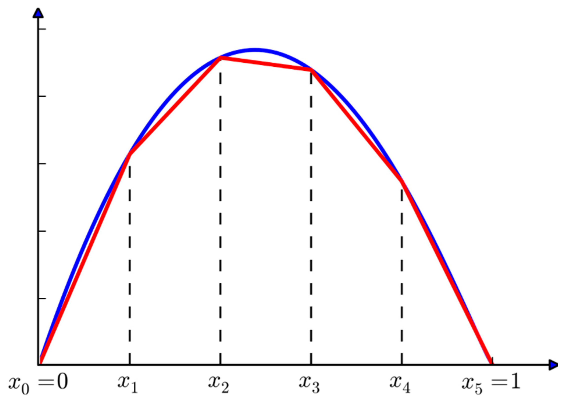
3.1. Piecewise Linear Approximation

In many studies over the past decades, piecewise linear approximation (PLA) techniques have been used to convert the non-linear LP models into their linear forms or mixed-integer convex optimization problems to obtain approximate global optimal solutions. To reformulate the original non-linear optimization problem, new variables of binary and continuous nature along with extra constraints are generally applied in the transformation process. The additional variables and constraint sets typically improve the effectiveness of obtaining solutions for the converted problem. The next sections of the manuscript present an overview of common PLAs and analyze their computational efficiency.

3.1.1. Formulations

Consider a general non-linear function $f\left(x\right)$ of a single variable $x,$ which is within the interval $\left[a_0,a_n\right]$. Such a continuous function has the advantage that we can approximate its non-linear expressions to piecewise linear ones as commonly used in the non-linear programming literature [59,60,61,62]. For comparing PLA techniques, interested readers can refer to the computational results reported by Li et al. [59] and Lin et al. [63].

• Method 1

First, divide $f\left(x\right)$ into n separate segments and define $a_i$ ($i\in \left\{0,1,\dots ,n\right\}$) as the breakpoints of $f\left(x\right)$, $a_0<a_1<\dots <a_n$. Then, we can approximately linearize the non-linear function $f\left(x\right)$ over the interval $\left[a_0,a_n\right]$ as follows:

$$L\left(f\left(x\right)\right)={\displaystyle {\displaystyle \sum }_{i=0}^n}f\left(a_i\right)·y_i,$$

(105)

$$s.t.$$

$${\displaystyle {\displaystyle \sum }_{i=0}^n}{a}_i·y_i=x,$$

(106)

$${\displaystyle {\displaystyle \sum }_{i=0}^n}{y}_i=1,$$

(107)

$$y_0\le t_0,$$

(108)

$$y_i\le t_{i-1}+t_i,\forall i\in \left\{1,\dots ,n-1\right\},$$

(109)

$$y_n\le t_{n-1},$$

(110)

$${\displaystyle {\displaystyle \sum }_{i=0}^{n-1}}{t}_i=1,$$

(111)

$$t_i\in \left\{0,1\right\},\forall i\in \left\{0,\dots ,n-1\right\},$$

(112)

$$y_i\in {ℝ}^{+},\forall i\in \left\{0,\dots ,n\right\}.$$

(113)

where only two adjacent $y_i$ are allowed to be non-zero.

Figure 4 illustrates the piecewise linearization of $f\left(x\right)$. The above terms include $n$ extra binary variables $t_0,t_1,\dots ,t_{n-1}$ and $n+1$ new continuous variables $y_0,y_1,\dots ,y_n$. The number of these newly added variables increases with the number of breakpoints ($n+1$), which leads to an exponential increase in computational time. The more linear segments there are, the more accurate the approximation will be at the expense of increasing the computational complexity.

• Method 2

Li and Yu [64] introduced a method for the global optimization of non-linear mathematical models in which the objective along with the constraint sets may be non-convex. First, a univariate mathematical function is formulated via a piecewise linear function using a sum of absolute expressions. Denote $s_i$ ($i\in \left\{0,1,\dots ,n-1\right\}$) as the slopes of each line between $a_i$ and $a_{i+1}$, computed using Equation (114):

$$s_i=\frac{f\left(a_{i+1}\right)-f\left(a_i\right)}{a_{i+1}-a_i},\forall i\in \left\{0,\dots ,n-1\right\}.$$

(114)

An equivalent piecewise linear form of non-linear function $f\left(x\right)$ can then be reformulated as follows:

$$L\left(f\left(x\right)\right)=f\left(a_0\right)+s_0·\left(x-a_0\right)+{\displaystyle {\displaystyle \sum }_{i=1}^{n-1}}\frac{s_i-s_{i-1}}{2}·\left(\left|x-a_i\right|+x-a_i\right).$$

(115)

If the successive slopes of the PLA are non-decreasing ($s_i-s_{i-1}\ge 0$) in the interval $\left[a_{i-1},a_i\right]$, $f\left(x\right)$ is convex. Otherwise, $f\left(x\right)$ is a concave (non-convex) function when these slopes are increasing. After linearization of the absolute term, Li and Yu [64] included additional binary variables $t_i$ to convert the non-convex model to a piecewise linear form as follows:

$$\begin{gathered} L\left(f\left(x\right)\right)=f\left(a_0\right)+s_0·\left(x-a_0\right)+{\displaystyle \sum }_{i:s_i>s_{i-1}}\left(s_i-s_{i-1}\right)·\left(x-a_i+{\displaystyle {\displaystyle \sum }_{j=0}^{i-1}}{d}_j\right) \\ +\frac{1}{2}{\displaystyle \sum }_{i:s_i<s_{i-1}}\left(s_i-s_{i-1}\right)·\left(x-a_i+2·a_i·t_i-2·z_i\right), \end{gathered}$$

(116)

$$s.t.$$

$$x+{\displaystyle {\displaystyle \sum }_{i=0}^{n-2}}{d}_i\ge a_{n-1},$$

(117)

$$d_i\le a_{i+1}-a_i,\forall i\in \left\{0,\dots ,n-1\right\}\mathrm{and}{s}_i>s_{i-1},$$

(118)

$$x+u\left(t_i-1\right)\le z_i,\forall i\in \left\{0,\dots ,n-1\right\}\mathrm{and}{s}_i<s_{i-1},$$

(119)

$$t_i\in \left\{0,1\right\},\forall i\in \left\{0,\dots ,n-1\right\},$$

(120)

$$d_i,z_i\in {ℝ}^{+},\forall i\in \left\{0,\dots ,n-1\right\}.$$

(121)

where $u$ is the upper bound of $x$.

Compared to Method 1, which used binary variables for all parts, the binary variables applied by the second approach have only been used to linearize the non-convex intervals of $f\left(x\right)$. Thus, the second method generally employs fewer binary variables than Method 1.

• Method 3

Another representing form of the piecewise approximating function has been used in the studies conducted by Li and Tsai [65], Topaloglu and Powell [66], Padberg [67], Li [68], and Croxton et al. [69]. The equivalent function can be formulated as demonstrated below.

$$x\ge a_i-\left(a_n-a_0\right)\left(1-t_i\right),\forall i\in \left\{0,\dots ,n-1\right\},$$

(122)

$$x\le a_{i+1}+\left(a_n-a_0\right)\left(1-t_i\right),\forall i\in \left\{0,\dots ,n-1\right\},$$

(123)

$$f\left(x\right)\ge f\left(a_i\right)+s_i·\left(x-a_i\right)-m\left(1-t_i\right),\forall i\in \left\{0,\dots ,n-1\right\},$$

(124)

$$f\left(x\right)\le f\left(a_i\right)+s_i·\left(x-a_i\right)+m\left(1-t_i\right),\forall i\in \left\{0,\dots ,n-1\right\},$$

(125)

$$s_i=\frac{f\left(a_{i+1}\right)-f\left(a_i\right)}{a_{i+1}-a_i},\forall i\in \left\{0,\dots ,n-1\right\},$$

(126)

$${\displaystyle {\displaystyle \sum }_{i=0}^{n-1}}{t}_i=1,$$

(127)

$$t_i\in \left\{0,1\right\},\forall i\in \left\{0,\dots ,n-1\right\}.$$

(128)

where $m$ is a sufficiently large constant.

When $n+1$ breakpoints are used, the above approach requires extra $n$ binary variables and $4n$ new constraint sets to model a piecewise linear function.

• Method 4

More linear pieces in the piecewise linear programming enhance the accuracy of the approximating function, but in the meantime, the execution time is negatively affected. To decrease the number of new binary variables added throughout the process of approximation, Li et al. [70] proposed a piecewise linearization technique that contains a logarithmic number of variables with binary nature in $n$. Consider the same continuous function $f\left(x\right)$ expressed above, where $x$ is assumed to be within the interval $\left[a_0,a_n\right]$ with $n+1$ breakpoints. Let $k$ be a positive integer number that can be represented using the following form:

$$k={\displaystyle {\displaystyle \sum }_{i=0}^{h-1}}{2}^i·y_i,$$

(129)

where $y_i$ are binary variables, $n-1$ denotes the upper bound of $k$, and $h$ is set to $\lfloor {\log }_2\left(n+1\right)\rfloor$.

Consider a set $A\left(k\right)\subseteq \left\{0,1,\dots ,h-1\right\}$ such that

$$k={\displaystyle \sum }_{i\in A\left(k\right)}{2}^i.$$

(130)

For example, $A\left(0\right)=\varnothing$, $A\left(3\right)=\left\{0,1\right\}$, and $A\left(5\right)=\left\{0,2\right\}$. Denote $\Vert A\left(k\right)\Vert$ to be the amount of elements in $A\left(k\right)$. For example, $\Vert A\left(0\right)\Vert =0$, and $\Vert A\left(3\right)\Vert =2$. Li et al. [70] proposed the following expressions for approximation of a univariate non-linear function:

$$L\left(f\left(x\right)\right)={\displaystyle {\displaystyle \sum }_{k=0}^{n-1}}\left(f\left(a_k\right)-s_k\left(a_k-a_0\right)\right)·r_k+{\displaystyle {\displaystyle \sum }_{k=0}^{n-1}}{s}_k·w_k,$$

(131)

$$s.t.$$

$$x\ge {\displaystyle {\displaystyle \sum }_{k=0}^{n-1}}{r}_k·a_k,$$

(132)

$$x\le {\displaystyle {\displaystyle \sum }_{k=0}^{n-1}}{r}_k·a_{k+1},$$

(133)

$$s_k=\frac{f\left(a_{k+1}\right)-f\left(a_k\right)}{a_{k+1}-a_k},\forall k\in \left\{0,\dots ,n-1\right\},$$

(134)

$${\displaystyle {\displaystyle \sum }_{k=0}^{n-1}}{r}_k=1,$$

(135)

$${\displaystyle {\displaystyle \sum }_{k=0}^{n-1}}{r}_k·\Vert A\left(k\right)\Vert +{\displaystyle {\displaystyle \sum }_{i=0}^{h-1}}{z}_i=0,$$

(136)

$$z_i\ge -y_i,\forall i\in \left\{0,\dots ,h-1\right\},$$

(137)

$$z_i\le y_i,\forall i\in \left\{0,\dots ,h-1\right\},$$

(138)

$$z_i\ge {\displaystyle {\displaystyle \sum }_{k=0}^{n-1}}{r}_k·c_{ki}-\left(1-y_i\right),\forall i\in \left\{0,\dots ,h-1\right\},$$

(139)

$$z_i\le {\displaystyle {\displaystyle \sum }_{k=0}^{n-1}}{r}_k·c_{ki}+\left(1-y_i\right),\forall i\in \left\{0,\dots ,h-1\right\},$$

(140)

$${\displaystyle {\displaystyle \sum }_{k=0}^{n-1}}{w}_k=x-a_0,$$

(141)

$${\displaystyle {\displaystyle \sum }_{k=0}^{n-1}}{w}_k·\Vert A\left(k\right)\Vert +{\displaystyle {\displaystyle \sum }_{i=0}^{h-1}}{v}_i=0,$$

(142)

$$v_i\ge -\left(a_n-a_0\right)·y_i,\forall i\in \left\{0,\dots ,h-1\right\},$$

(143)

$$v_i\le \left(a_n-a_0\right)·y_i,\forall i\in \left\{0,\dots ,h-1\right\},$$

(144)

$$v_i\ge {\displaystyle {\displaystyle \sum }_{k=0}^{n-1}}{w}_k·c_{ki}-\left(a_n-a_0\right)·\left(1-y_i\right),\forall i\in \left\{0,\dots ,h-1\right\},$$

(145)

$$v_i\le {\displaystyle {\displaystyle \sum }_{k=0}^{n-1}}{w}_k·c_{ki}+\left(a_n-a_0\right)·\left(1-y_i\right),\forall i\in \left\{0,\dots ,h-1\right\},$$

(146)

$$y_i\in \left\{0,1\right\},\forall i\in \left\{0,\dots ,h-1\right\},$$

(147)

$$r_k,w_k\in {ℝ}^{+},\forall k\in \left\{0,\dots ,n-1\right\},$$

(148)

$$c_{ki},z_i,v_i\in ℝ,\forall k\in \left\{0,\dots ,n-1\right\},\forall i\in \left\{0,\dots ,h-1\right\}.$$

(149)

Considering $n+1$ breakpoints, this method requires $h$ binary variables, $2n$ non-negative variables, and $h·\left(n+1\right)$ free-signed continuous variables. Although the method proposed by Li et al. [70] uses fewer variables of binary nature, Vielma et al. [71] showed that this approach is not a theoretically and computationally superior representation method for piecewise linear functions.

• Method 5

To approximate the non-linear functions of a variable, Vielma and Nemhauser [72] developed a new expression that needs fewer variables and constraints than previous representation methods. Their formulation requires a logarithmic number of binary variables and constraint sets in expressing a piecewise approximating function as follows. Let $i\in I=\left\{0,1,\dots ,n\right\}$ and $B\left(i\right)=\left(y_1,y_2,\dots ,y_h\right)$, where $h=\lceil {\log }_{2}n\rceil$, $y_k\in \left\{0,1\right\}$ for $k\in \left\{1,\dots ,h\right\}$. Let $B:\left\{0,1,\dots ,n\right\}\to {\left\{0,1\right\}}^h$ denote the injective function, where the vectors $B\left(i\right)$ and $B\left(i+1\right)$ differ in at most one component for all $i\in \left\{1,\dots ,n-1\right\}$ and $B\left(0\right)=B\left(1\right)$. Let $S^{+}\left(k\right)$ be a set of $i$ where $y_k=1$ in both $B\left(i\right)$ and $B\left(i+1\right)$ for $i\in \left\{1,\dots ,n-1\right\}$ or just in $B\left(i\right)$ for $i\in \left\{0,n\right\}$ ($S^{+}\left(k\right)=\left\{i|B\left(i\right)\mathrm{and}B\left(i+1\right)\forall i\in \left\{1,\dots ,n-1\right\}:y_k=1\right\}{\displaystyle \cup }\left\{i|B\left(i\right)\forall i\in \left\{0,n\right\}:y_k=1\right\}$). Let $S^{-}\left(k\right)$ be a set of $i$ where $y_k=0$ in both $B\left(i\right)$ and $B\left(i+1\right)$ for $i\in \left\{1,\dots ,n-1\right\}$ or just in $B\left(i\right)$ for $i\in \left\{0,n\right\}$ ($S^{+}\left(k\right)=\left\{i|B\left(i\right)\mathrm{and}B\left(i+1\right)\forall i\in \left\{1,\dots ,n-1\right\}:y_k=0\right\}{\displaystyle \cup }\left\{i|B\left(i\right)\forall i\in \left\{0,n\right\}:y_k=0\right\}$). The piecewise linear function of $f\left(x\right)$ with $n+1$ breakpoints where $a_0<a_1<\dots <a_n$ can be represented as:

$$L\left(f\left(x\right)\right)={\displaystyle {\displaystyle \sum }_{i=0}^n}f\left(a_i\right)·{\lambda }_i,$$

(150)

$$s.t.$$

$$x={\displaystyle {\displaystyle \sum }_{i=0}^n}{a}_i·{\lambda }_i,$$

(151)

$${\displaystyle {\displaystyle \sum }_{i=0}^n}{\lambda }_i=1,$$

(152)

$${\displaystyle \sum }_{i\in S^{+}\left(k\right)}{\lambda }_i\le y_k,\forall k\in \left\{1,\dots ,h\right\},$$

(153)

$${\displaystyle \sum }_{i\in S^{-}\left(k\right)}{\lambda }_i\le 1-y_k,\forall k\in \left\{1,\dots ,h\right\},$$

(154)

$$y_k\in \left\{0,1\right\},\forall k\in \left\{1,\dots ,h\right\},$$

(155)

$${\lambda }_i\in {ℝ}^{+},\forall i\in \left\{0,\dots ,n\right\}.$$

(156)

To form a piecewise linear programming function with $n$ pieces, this method applies $\lceil {\log }_{2}n\rceil$ variables of binary nature, $n+1$ variables of continuous nature, and $2+2·\lceil {\log }_{2}n\rceil$ constraint sets. Method 5 induces a piecewise linear function with an independent branching scheme of logarithm depth and constructs a tighter convex estimator, making fewer breakpoints to meet the feasibility and optimality tolerance. Experimental results from the literature [71,73] show that this method provides a significant computational advantage in the linearization process and outperforms other methods, especially when more breakpoints are used.

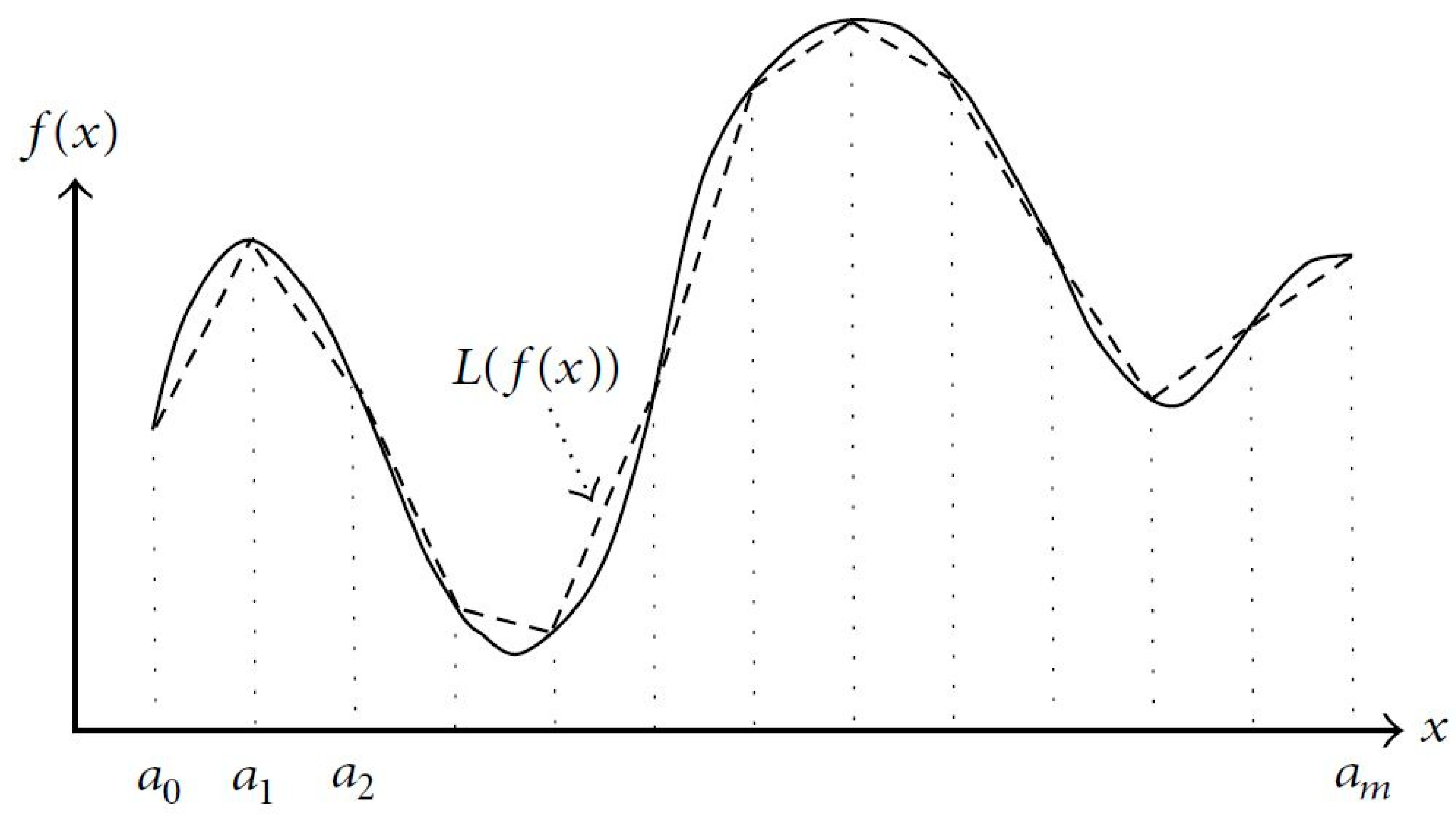
3.1.2. PLA-Based Algorithms

Establishing the PLA generates its own optimization problem. To properly fit a curve, the most accurate PLA uses an infinite amount of segments. The complexity associated with this procedure becomes similar to the initial non-linear model. In solving the new decision problem, the main goal is to determine the best approximation with the least number of linear pieces. There are a number of commercial solvers, such as MINOS and CONOPT used within the General Algebraic Modeling System (GAMS), that can solve these problems [74]. There are also several optimal search algorithms using PLAs to solve complicated models with both concave and convex objective functions [75,76,77,78]. The most prominent algorithms developed based on PLA techniques include the following:

• Approximating Planar Curves

PLAs are not just restricted to two-dimensional cases but can be utilized to fit multi-dimensional planes and curves. Williams [79] presented the first algorithm that efficiently fits flat curves by using the required number of linear vectors. The proposed methodology of approximating the fitting of straight lines to a plane is based on the geometric analysis of the curvature of the plane, with subsequent geometrically accurate and numerically stable calculations.

• Single Pass PLA Algorithm

Gritzali and Papakonstantinou [80] devised an algorithm for finding different parts of a formulated waveform function and identifying a number of peak points. The points marked as peaks are those where the derivative of the function equals zero. This algorithm starts with a maximum point plotted on the piecewise curve and develops the PLA into the function in order that all points on the waveform have the same difference with respect to the piecewise approximation. Such an algorithm can obviously be beneficial in real-time applications like an electrocardiogram readout where peaks are important.

• Branch and Refine

The branching and refining algorithm is based on the well-known PLA techniques. This is an effective way to find a global optimum for a non-linear problem. The algorithm applies PLAs to determine global lower bounds for mixed-integer non-linear optimization models, and from there, the upper bounds of the problem are provided by the feasible solutions. As the amount of iterations increases, the amount of segments increases, and the algorithm moves towards the global solution. For more information regarding the branching and refining algorithm, the interested readers can refer to Leyffer et al. [81] and Gong and You [82].

• PLAs for Accuracy

The algorithm designed by Nishikawa [83] estimates the global and local asymptotic $L_2$ error as a piecewise continuous linear approximation in a manner that the target error on the curve can be achievable. The latter task can be accomplished via the local error analysis, which is followed by using key terms for the approximation. Some numerical tests are then performed to verify that the error is around $L_2$.

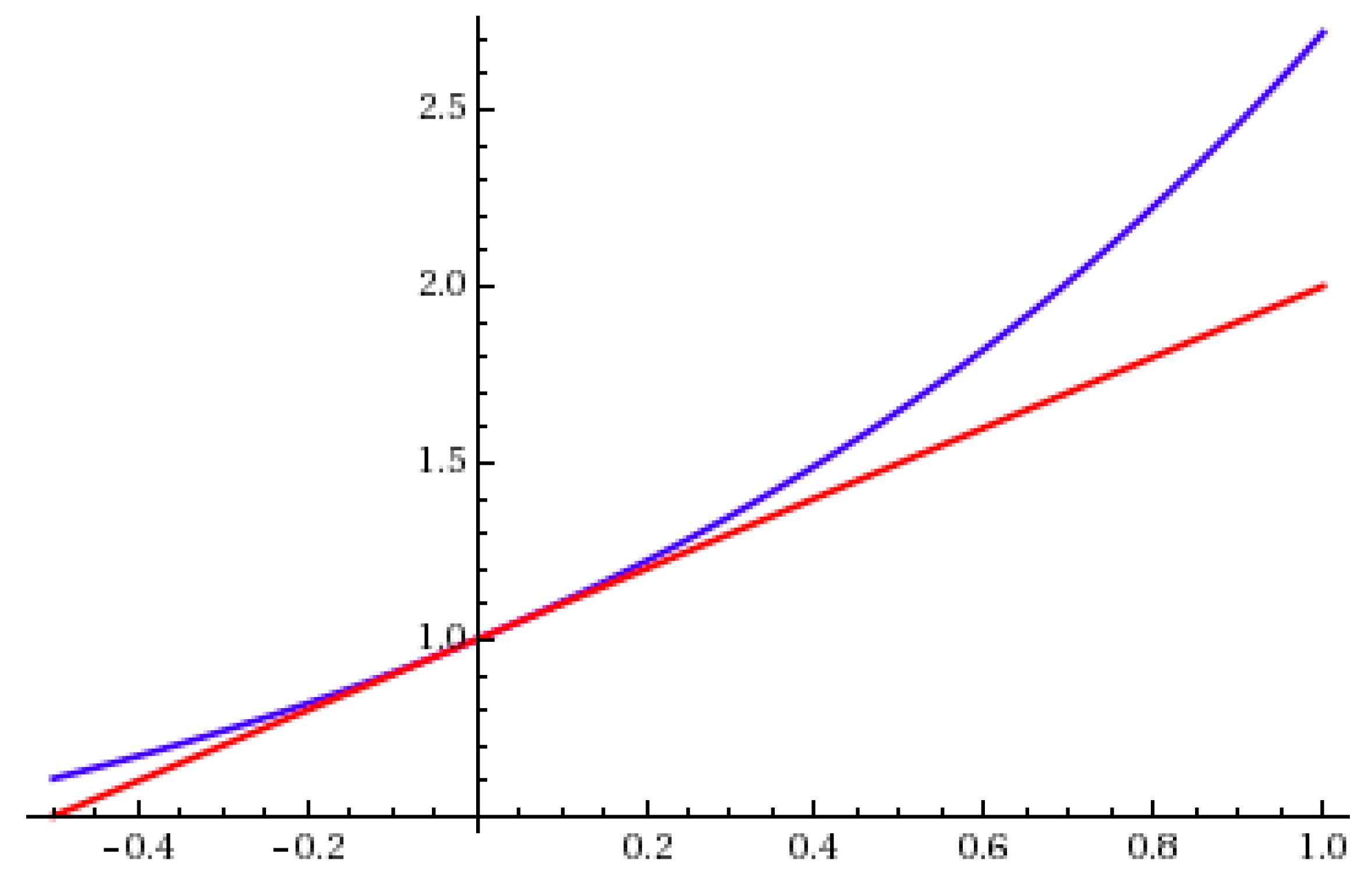
3.2. Log-Linearization via Taylor Series Approximation

There exist many different types of non-linear problems (e.g., dynamic stochastic general equilibrium), for which there exist no closed-form solutions and solving these problems is challenging. The log-linearization approach can be applied for such cases. When using the log-linearization approach, it is necessary to approximate the non-linear equations characterizing the equilibrium with log-linear ones. The strategy is to first take the natural logs of the non-linear equations and then use the first-order Taylor approximation around the steady-state to replace the logged difference equations with linear approximations in the log-deviations of the variables. There are different ways to perform log-linearization [84,85,86]. One of the main theories is to apply the Taylor Series expansion as suggested by Griffith and Stewart [87]. Taylor’s theorem indicates that the first-order approximation of an arbitrary mathematical function $f\left(x\right)$ centered at $x=x^{*}$ (differentiable $n$ times at some point $x^{*}$) can be represented as follows:

$$f\left(x\right)\cong f\left(x^{*}\right)+f^{\prime }\left(x^{*}\right)·\left(x-x^{*}\right).$$

(157)

For example, the function $f\left(x\right)=\ln \left(1+x\right)$ can be approximated at $x=2$ by the first-order Taylor polynomial as follows:

$$f\left(x\right)\cong \ln 3+\frac{1}{3}·\left(x-2\right)=0.43195+0.3333·x.$$

(158)

The first-order Taylor approximations can also be used to convert equations with more than one endogenous variable to a log-deviation form. The first-order Taylor polynomial of the function $f\left(x,y\right)$ at the steady-state values $x=x^{*}$ and $y=y^{*}$ gives

$$f\left(x,y\right)\cong f\left(x^{*},y^{*}\right)+{\displaystyle f_x^{\prime }}\left(x^{*},y^{*}\right).\left(x-x^{*}\right)+{\displaystyle f_y^{\prime }}\left(x^{*},y^{*}\right)·\left(y-y^{*}\right).$$

(159)

This methodology could be used to log-linearize equations and take the log-deviation around the steady state-value. Log-linearization means around a steady state. The log-deviation of the variable $x$ from its steady state $x^{*}$ is defined as

$$\tilde{x}=\ln x-\ln x^{*}.$$

(160)

The right-hand side of Equation (160) can be rewritten as

$$\ln \left(\frac{x}{x^{*}}\right)=\ln \left(1+\frac{x-x^{*}}{x^{*}}\right).$$

(161)

Using the first-order Taylor polynomial mentioned in Equation (157), the log expression can be approximated at the steady state $x=x^{*}$ as

$$\ln \left(1+\frac{x-x^{*}}{x^{*}}\right)\cong \ln 1+\frac{1}{x^{*}}·\left(x-x^{*}\right).$$

(162)

Thus, we get log-deviation of $x$ about $x^{*}$ as

$$\tilde{x}=\frac{x-x^{*}}{x^{*}}.$$

(163)

Consider an example of the Cobb-Douglas production function $y_t=a_t·{\displaystyle k_t^{\alpha }}·{\displaystyle n_t^{1-\alpha }}$ and then take a log of the function:

$$\ln y_t=\ln a_t+\alpha ·\ln k_t+\left(1-\alpha \right)·\ln n_t.$$

(164)

Using Taylor Series expansion is the next step, we take the first order approximation as follows:

$$\begin{array}{l}\ln y^{*}+\frac{1}{y^{*}}·\left(y_t-y^{*}\right)\\ =\ln a^{*}+\frac{1}{a^{*}}·\left(a_t-a^{*}\right)+\alpha ·\ln k^{*}+\frac{\alpha }{k^{*}}·\left(k_t-k^{*}\right)+\left(1-\alpha \right)·\ln n^{*}\\ +\frac{1-\alpha }{n^{*}}·\left(n_t-n^{*}\right).\end{array}$$

(165)

Since $\ln y^{*}=\ln a^{*}+\alpha ·\ln k^{*}+\left(1-\alpha \right)·\ln n^{*}$, we can cancel out the relevant parts of the approximation, which will result in the following expression:

$$\frac{1}{y^{*}}·\left(y_t-y^{*}\right)=\frac{1}{a^{*}}·\left(a_t-a^{*}\right)+\frac{\alpha }{k^{*}}·\left(k_t-k^{*}\right)+\frac{1-\alpha }{n^{*}}·\left(n_t-n^{*}\right).$$

(166)

For notational ease, the equations are defined as the percentage deviation about the steady-state. Thus, applying log-deviation stated in Equation (163) to this approximation leads to

$${\tilde{y}}_t={\tilde{a}}_t+\alpha ·{\tilde{k}}_t+\left(1-\alpha \right)·{\tilde{n}}_t.$$

(167)

The method of taking logs and then subtracting the log terms from the steady-state equation is very convenient. However, it does not always work. It is only useful for multiplicative equations or when the log removes exponents and converts multiplication into addition to significantly simplify the equation. However, the method of taking logs and then subtracting the log terms from the steady-state equation should not be used for the equations that involve expectation terms, even when the equation is multiplicative [85]. This is because taking the expectation of a logarithmic term is not the same as taking the log from the expectation term.

4. Conclusions

In this study, a comprehensive and holistic review of transformation and linearization techniques was provided to deal with non-linear terms in optimization models. The following groups of operations research techniques for solving optimization problems with non-linear terms were analyzed: (i) transformations in which the non-linear equations or functions are replaced by an exact equivalent linear programming (LP) formulation to create valid inequalities; and (ii) linear approximations which find the equivalent of a non-linear function with the least deviation around the point of interest or separate straight-line segments. The existing transformation approaches for different scenarios were considered, including the multiplication of binary variables, multiplication of binary and continuous variables, multiplication of continuous variables, maximum/minimum operators, absolute value function, floor and ceiling functions, square root function, and multiple breakpoint function. As for linear approximations, the present survey provided a detailed review of piecewise approximating functions and log-linearization via Taylor series approximation.

The main advantages and disadvantages of using common transformation and linearization techniques were investigated as a part of this survey as well. Along with a review of the existing methods, this study proposed a new technique for linearizing the square root terms by means of transformation to obtain tight LP relaxations. Furthermore, a new approach was presented to incorporate quadratic integers into LP mathematical formulations. The aforementioned contributions are expected to enhance the solvability of optimization models with non-linear terms and, ultimately, facilitate decision making. Furthermore, the information presented in this survey study can be used by scientists and practitioners, who often work with optimization models that have non-linear terms, and selection of the appropriate transformation and linearization techniques. In conclusion, a detailed review of the relevant literature confirms that transformation methods were found be efficient, as they ensure model feasibility and allow reducing the computation time.

The scope of future research for this study can focus more on additional techniques that can be used to decrease computational time even further after transformation of the original optimization model into its linear form (e.g., Lagrangian relaxation, Benders decomposition). Furthermore, a number of iterative optimization algorithms that directly rely on linearization techniques have been applied in the literature for different decision problems [88,89,90]. Another interesting research direction would be the investigation of computational complexity changes due to the deployment of linearization techniques in such algorithms. Moreover, future research can compare the computational performance of various PLA techniques in more detail for different scenarios. Last but not least, the future research can concentrate more on different domains where transformation and linearization techniques have been applied the most to discover additional tendencies and potential implementation challenges.

References

1. Negrello, C.; Gosselet, P.; Rey, C. Nonlinearly Preconditioned FETI Solver for Substructured Formulations of Nonlinear Problems. Mathematics 2021, 9, 3165. [Google Scholar] [CrossRef]
2. Petridis, K.; Drogalas, G.; Zografidou, E. Internal auditor selection using a TOPSIS/non-linear programming model. Ann. Oper. Res. 2021, 296, 513–539. [Google Scholar] [CrossRef]
3. Stoyan, Y.; Yaskov, G. Optimized packing unequal spheres into a multiconnected domain: Mixed-integer non-linear programming approach. Int. J. Comput. Math. Comput. Syst. Theory 2021, 6, 94–111. [Google Scholar] [CrossRef]
4. Dulebenets, M.A. The vessel scheduling problem in a liner shipping route with heterogeneous fleet. Int. J. Civ. Eng. 2018, 16, 19–32. [Google Scholar] [CrossRef]
5. Fathollahi-Fard, A.M.; Hajiaghaei-Keshteli, M.; Tavakkoli-Moghaddam, R.; Smith, N.R. Bi-level programming for home health care supply chain considering outsourcing. J. Ind. Inf. Integr. 2021, 25, 100246. [Google Scholar] [CrossRef]
6. Bertsimas, D.; Dunn, J.; Wang, Y. Near-optimal nonlinear regression trees. Oper. Res. Lett. 2021, 49, 201–206. [Google Scholar] [CrossRef]
7. Fathollahi-Fard, A.M.; Woodward, L.; Akhrif, O. Sustainable distributed permutation flow-shop scheduling model based on a triple bottom line concept. J. Ind. Inf. Integr. 2021, 24, 100233. [Google Scholar] [CrossRef]
8. Pauer, G.; Török, Á. Binary integer modeling of the traffic flow optimization problem, in the case of an autonomous transportation system. Oper. Res. Lett. 2021, 49, 136–143. [Google Scholar] [CrossRef]
9. Guignard, M. Strong RLT1 bounds from decomposable Lagrangean relaxation for some quadratic 0–1 optimization problems with linear constraints. Ann. Oper. Res. 2020, 286, 173–200. [Google Scholar] [CrossRef]
10. Hsu, H.-P.; Wang, C.-N.; Fu, H.-P.; Dang, T.-T. Joint Scheduling of Yard Crane, Yard Truck, and Quay Crane for Container Terminal Considering Vessel Stowage Plan: An Integrated Simulation-Based Optimization Approach. Mathematics 2021, 9, 2236. [Google Scholar] [CrossRef]
11. Dulebenets, M.A. Advantages and disadvantages from enforcing emission restrictions within emission control areas. Marit. Bus. Rev. 2016, 1, 107–132. [Google Scholar] [CrossRef] [Green Version]
12. Pasha, J.; Dulebenets, M.A.; Kavoosi, M.; Abioye, O.F.; Theophilus, O.; Wang, H.; Kampmann, R.; Guo, W. Holistic tactical-level planning in liner shipping: An exact optimization approach. J. Shipp. Trade 2020, 5, 8. [Google Scholar] [CrossRef]
13. Dulebenets, M.A. A comprehensive multi-objective optimization model for the vessel scheduling problem in liner shipping. Int. J. Prod. Econ. 2018, 196, 293–318. [Google Scholar] [CrossRef]
14. Cameron, S.H. Piece-wise linear approximations. In Technical Report CSTN-106; Computer Science Division, IIT Research Institute: Chicago, IL, USA, 1966. [Google Scholar]
15. Bradley, S.P.; Hax, A.C.; Magnanti, T.L. Applied Mathematical Programming; Addison-Wesley: Reading, MA, USA, 1977. [Google Scholar]
16. Gajjar, H.K.; Adil, G.K. A piecewise linearization for retail shelf space allocation problem and a local search heuristic. Ann. Oper. Res. 2010, 179, 149–167. [Google Scholar] [CrossRef]
17. Geißler, B.; Martin, A.; Morsi, A.; Schewe, L. Using piecewise linear functions for solving MINLPs. In Mixed Integer Nonlinear Programming; Lee, J., Leyffer, S., Eds.; Springer: New York, NY, USA, 2012; Volume 154, pp. 287–314. [Google Scholar]
18. Sridhar, S.; Linderoth, J.; Luedtke, J. Locally ideal formulations for piecewise linear functions with indicator variables. Oper. Res. Lett. 2013, 41, 627–632. [Google Scholar] [CrossRef] [Green Version]
19. Andrade-Pineda, J.L.; Canca, D.; Gonzalez-R, P.L. On modelling non-linear quantity discounts in a supplier selection problem by mixed linear integer optimization. Ann. Oper. Res. 2017, 258, 301–346. [Google Scholar] [CrossRef]
20. Stefanello, F.; Buriol, L.S.; Hirsch, M.J.; Pardalos, P.M.; Querido, T.; Resende, M.G.C.; Ritt, M. On the minimization of traffic congestion in road networks with tolls. Ann. Oper. Res. 2017, 249, 119–139. [Google Scholar] [CrossRef]
21. Meyer, R.R.A. Theoretical and computational comparison of ‘Equivalent’ mixed-integer formulations. Nav. Res. Logist. 1981, 28, 115–131. [Google Scholar] [CrossRef] [Green Version]
22. Jeroslow, R.G.; Lowe, J.K. Modeling with integer variables. In Mathematical Programming at Oberwolfach II. Mathematical Programming Studies; Korte, B., Ritter, K., Eds.; Springer: Berlin/Heidelberg, Germany, 1984; Volume 22. [Google Scholar]
23. Jeroslow, R.G.; Lowe, J.K. Experimental results on new techniques for integer programming formulations. J. Oper. Res. Soc. 1985, 36, 393–403. [Google Scholar] [CrossRef]
24. Balas, E. Disjunctive programming and a hierarchy of relaxations for discrete optimization problems. SIAM J. Algebraic Discret. Methods 1985, 6, 466–486. [Google Scholar] [CrossRef]
25. Johnson, E.L. Modeling and Strong Linear Programs for Mixed Integer Programming. In Algorithms and Model Formulations in Mathematical Programming; NATO ASI Series (Series F: Computer and Systems Sciences); Wallace, S.W., Ed.; Springer: Berlin/Heidelberg, Germany, 1989; Volume 51. [Google Scholar]
26. Wolsey, L.A. Strong formulations for mixed integer programming: A survey. Math. Program. 1989, 45, 173–191. [Google Scholar] [CrossRef]
27. Sherali, H.D.; Adams, W.P. A hierarchy of relaxations between the continuous and convex hull representations for zero-one programming problems. SIAM J. Discret. Math. 1990, 3, 411–430. [Google Scholar] [CrossRef]
28. Sherali, H.D.; Adams, W.P. A hierarchy of relaxations and convex hull characterizations for mixed-integer zero-one programming problems. Discret. Appl. Math. 1994, 52, 83–106. [Google Scholar] [CrossRef] [Green Version]
29. Williams, H.P. Model Building in Mathematical Programming, 5th ed.; WILEY: Hoboken, NJ, USA, 2013. [Google Scholar]
30. Glover, F. Improved linear integer programming formulations of nonlinear integer problems. Manag. Sci. 1975, 22, 455–460. [Google Scholar] [CrossRef] [Green Version]
31. Balas, E.; Mazzola, J.B. Nonlinear 0-1 programming: I. Linearization techniques. Math. Program. 1984, 30, 2–12. [Google Scholar] [CrossRef]
32. Balas, E.; Mazzola, J.B. Nonlinear 0-1 programming: II. Dominance relations and algorithms. Math. Program. 1984, 30, 22–45. [Google Scholar] [CrossRef]
33. Adams, W.P.; Sherali, H.D. A tight linearization and an algorithm for zero-one quadratic programming problems. Manag. Sci. 1986, 32, 1274–1290. [Google Scholar] [CrossRef]
34. Adams, W.P.; Sherali, H.D. Linearization strategies for a class of zero-one mixed integer programming problems. Oper. Res. 1990, 38, 217–226. [Google Scholar] [CrossRef]
35. Adams, W.P.; Sherali, H.D. Mixed-integer bilinear programming problems. Math. Program. 1993, 59, 279–305. [Google Scholar] [CrossRef]
36. Adams, W.P.; Billionnet, A.; Sutter, A. Unconstrained 0-1 optimization and lagrangean relaxation. Discret. Appl. Math. 1990, 29, 131–142. [Google Scholar] [CrossRef] [Green Version]
37. Bisschop, J. AIMMS Optimization Modeling. 2021. Available online: https://documentation.aimms.com/aimms_modeling.html (accessed on 25 February 2021).
38. Rahil, A. Linearization of Mixed Integer Programming. 2012. Available online: www.iems.ucf.edu/qzheng/grpmbr/seminar/Anees_Linear_General_Slides.pdf (accessed on 25 February 2021).
39. Asghari, M.; Mirzapour Al-e-hashem, S.M.J. A Green Delivery-Pickup Problem for Home Hemodialysis Machines; Sharing Economy in Distributing Scarce Resources. Transp. Res. Part E 2020, 134, 101815. [Google Scholar] [CrossRef]
40. Asghari, M.; Mirzapour Al-e-hashem, S.M.J.; Rekik, Y. Environmental and social implications of incorporating carpooling service on a customized bus system. Comput. Oper. Res. 2022, in press. [Google Scholar]
41. Mojtahedi, M.; Fathollahi-Fard, A.M.; Tavakkoli-Moghaddam, R.; Newton, S. Sustainable vehicle routing problem for coordinated solid waste management. J. Ind. Inf. Integr. 2021, 23, 100220. [Google Scholar] [CrossRef]
42. Mohammadi, S.; Mirzapour Al-e-Hashem, S.M.J.; Rekik, Y. An integrated production scheduling and delivery route planning with multi-purpose machines: A case study from a furniture manufacturing company. Int. J. Prod. Econ. 2020, 219, 347–359. [Google Scholar] [CrossRef]
43. Mangasarian, O.L.; Meyer, R.R. Absolute value equations. Linear Algebra Appl. 2006, 419, 359–367. [Google Scholar] [CrossRef] [Green Version]
44. Mangasarian, O.L. Absolute value equation solution via concave minimization. Optim. Lett. 2007, 1, 3–8. [Google Scholar] [CrossRef]
45. Mangasarian, O.L. Absolute value programming. Comput. Optim. Appl. 2007, 36, 43–53. [Google Scholar] [CrossRef]
46. Mangasarian, O.L. A generalized Newton method for absolute value equations. Optim. Lett. 2009, 3, 101–108. [Google Scholar] [CrossRef]
47. Caccetta, L.; Qu, B.; Zhou, G. A globally and quadratically convergent method for absolute value equations. Comput. Optim. Appl. 2001, 48, 45–58. [Google Scholar] [CrossRef]
48. Boyd, S.; Vandenberghe, L. Convex Optimization; Cambridge University Press: Cambridge, UK, 2004. [Google Scholar]
49. Ferguson, R.O.; Sargent, L.A. Linear Programming: Fundamentals and Applications; Mc Graw-Hill Book Company: New York, NY, USA, 1958. [Google Scholar]
50. McCarl, B.A.; Spreen, T.H. Applied Mathematical Programming Using Algebraic Systems. 1997. Available online: http://agecon2.tamu.edu/people/faculty/mccarl-bruce/books.htm (accessed on 25 February 2021).
51. Gelfand, I.M.; Shen, A. Algebra. Springer Science & Business Media. Birkhäuser Boston, 2003. Available online: https://books.google.com/books?id=Z9z7iliyFD0C (accessed on 25 February 2021).
52. Kwon, T.J.; Draper, J. Floating-point division and square root using a Taylor-series expansion algorithm. Microelectron. J. 2009, 40, 1601–1605. [Google Scholar] [CrossRef] [Green Version]
53. Del Moral, P.; Niclas, A. A Taylor expansion of the square root matrix function. J. Math. Anal. Appl. 2018, 465, 259–266. [Google Scholar] [CrossRef]
54. Tsai, J.F. An optimization approach for supply chain management models with quantity discount policy. Eur. J. Oper. Res. 2007, 177, 982–994. [Google Scholar] [CrossRef]
55. Mirzapour Al-e-hashem, S.M.J.; Baboli, A.; Sazvar, Z. A stochastic aggregate production planning model in a green supply chain: Considering flexible lead times, nonlinear purchase and shortage cost functions. Eur. J. Oper. Res. 2013, 230, 26–41. [Google Scholar] [CrossRef]
56. Dembo, R.S. Current state of the art of algorithms and computer software for geometric programming. J. Optim. Theory Appl. 1978, 26, 149–183. [Google Scholar] [CrossRef]
57. McCarl, B.A.; Tice, T. Should Quadratic Programming Problems be Approximated? Am. J. Agric. Econ. 1982, 64, 585–589. [Google Scholar] [CrossRef]
58. McCarl, B.A.; Onal, H. Linear Approximation Using MOTAD and Separable Programming: Should it be Done? Am. J. Agric. Econ. 1989, 71, 158–166. [Google Scholar] [CrossRef]
59. Li, H.L.; Chang, C.T.; Tsai, J.F. Approximately global optimization for assortment problems using piecewise linearization techniques. Eur. J. Oper. Res. 2002, 140, 584–589. [Google Scholar] [CrossRef]
60. Bazaraa, M.S.; Sherali, H.D.; Shetty, C.M. Nonlinear Programming: Theory and Algorithms, 3rd ed.; Wiley-Interscience: New York, NY, USA, 2013. [Google Scholar]
61. Hillier, F.S.; Lieberman, G.J. Introduction to Operations Research, 9th ed.; McGraw-Hill: New York, NY, USA, 2009. [Google Scholar]
62. Taha, H.A. Operations Research an Introduction, 10th ed.; Prentice Hall: Upper Saddle River, NJ, USA, 2017. [Google Scholar]
63. Lin, M.H.; Carlsson, J.G.; Ge, D.; Shi, J.; Tsai, J.F. A Review of Piecewise Linearization Methods. Math. Probl. Eng. 2013, 2013, 101376. [Google Scholar] [CrossRef] [Green Version]
64. Li, H.L.; Yu, C.S. Global optimization method for nonconvex separable programming problems. Eur. J. Oper. Res. 1999, 117, 275–292. [Google Scholar] [CrossRef]
65. Li, H.L.; Tsai, J.F. Treating free variables in generalized geometric global optimization programs. J. Glob. Optim. 2005, 33, 1–13. [Google Scholar] [CrossRef]
66. Topaloglu, H.; Powell, W.B. An algorithm for approximating piecewise linear concave functions from sample gradients. Oper. Res. Lett. 2003, 31, 66–76. [Google Scholar] [CrossRef]
67. Padberg, M. Approximating separable nonlinear functions via mixed zero-one programs. Oper. Res. Lett. 2000, 27, 1–5. [Google Scholar] [CrossRef] [Green Version]
68. Li, H.L. An efficient method for solving linear goal programming problems. J. Optim. Theory Appl. 1996, 90, 465–469. [Google Scholar] [CrossRef]
69. Croxton, K.L.; Gendron, B.; Magnanti, T.L. A comparison of mixed-integer programming models for nonconvex piecewise linear cost minimization problems. Manag. Sci. 2003, 49, 1268–1273. [Google Scholar] [CrossRef] [Green Version]
70. Li, H.L.; Lu, H.C.; Huang, C.H.; Hu, N.Z. A superior representation method for piecewise linear functions. INFORMS J. Comput. 2009, 21, 314–321. [Google Scholar] [CrossRef]
71. Vielma, J.P.; Ahmed, S.; Nemhauser, G. A note on a superior representation method for piecewise linear functions. INFORMS J. Comput. 2010, 22, 493–497. [Google Scholar] [CrossRef] [Green Version]
72. Vielma, J.P.; Nemhauser, G. Modeling disjunctive constraints with a logarithmic number of binary variables and constraints. Math. Program. 2011, 128, 49–72. [Google Scholar] [CrossRef]
73. Tsai, J.F.; Lin, M.H. An efficient global approach for posynomial geometric programming problems. INFORMS J. Comput. 2011, 23, 483–492. [Google Scholar] [CrossRef]
74. Ahmadi, H.; Martí, J.R.; Moshref, A. Piecewise linear approximation of generators cost functions using max-affine functions. In Proceedings of the 2013 IEEE Power & Energy Society General Meeting, Vancouver, BC, Canada, 21–25 July 2013; pp. 1–5. [Google Scholar]
75. Ajili, F.; El Sakkout, H. A Probe-Based Algorithm for Piecewise Linear Optimization in Scheduling. Ann. Oper. Res. 2003, 118, 35–48. [Google Scholar] [CrossRef]
76. Keha, A.B.; De Farias, I.R.; Nemhauser, G.L. A branch-and-cut algorithm without binary variables for nonconvex piecewise linear optimization. Oper. Res. 2006, 54, 847–858. [Google Scholar] [CrossRef]
77. Imamoto, A.; Tang, B. Optimal piecewise linear approximation of convex functions. In Proceedings of the World Congress on Engineering and Computer Science, San Francisco, CA, USA, 22–24 October 2008; pp. 1191–1194. [Google Scholar]
78. Melo, W.; Fampa, M.; Raupp, F. Two linear approximation algorithms for convex mixed integer nonlinear programming. Ann. Oper. Res. 2020. [Google Scholar] [CrossRef]
79. Williams, C.M. An efficient algorithm for the piecewise linear approximation of planar curves. Comput. Graph. Image Process. 1978, 8, 286–293. [Google Scholar] [CrossRef]
80. Gritzali, F.; Papakonstantinou, G. A fast piecewise linear approximation algorithm. Signal Process. 1983, 5, 221–227. [Google Scholar] [CrossRef]
81. Leyffer, S.; Sartenaer, A.; Wanufelle, E. Branch-and-Refine for Mixed-Integer Nonconvex Global Optimization; ANL/MCS-P1547-0908; Argonne National Laboratory: Argonne, IL, USA, 2008; preprint.
82. Gong, J.; You, F. Global optimization for sustainable design and synthesis of algae processing network for CO2 mitigation and biofuel production using life cycle optimization. AIChE J. 2014, 60, 3195–3210. [Google Scholar] [CrossRef]
83. Nishikawa, H. Accurate Piecewise Linear Continuous Approximations to One-Dimensional Curves: Error Estimates and Algorithms; Department of Aerospace Engineering, University of Michigan: Ann Arbor, MI, USA, 1998. [Google Scholar]
84. Uhlig, H. A toolkit for analyzing nonlinear dynamic stochastic models easily. In Computational Methods for the Study of Dynamic Economies; Marimon, R., Scott, A., Eds.; Oxford University Press: New York, NY, USA, 1999; pp. 30–61. [Google Scholar]
85. Zietz, J. Log-Linearizing Around the Steady State: A Guide with Examples. Available online: https://ssrn.com/abstract=951753 (accessed on 25 February 2021).
86. McCandless, G. The ABCs of RBCs: An Introduction to Dynamic Macroeconomic Models; Harvard University Press: Cambridge, MA, USA, 2008. [Google Scholar]
87. Griffith, R.E.; Stewart, R.A. A Nonlinear Programming Technique for the Optimization of Continuous Processing Systems. Manag. Sci. 1961, 7, 379–392. [Google Scholar] [CrossRef]
88. Pasha, J.; Dulebenets, M.A.; Fathollahi-Fard, A.M.; Tian, G.; Lau, Y.Y.; Singh, P.; Liang, B. An integrated optimization method for tactical-level planning in liner shipping with heterogeneous ship fleet and environmental considerations. Adv. Eng. Inform. 2021, 48, 101299. [Google Scholar] [CrossRef]
89. Dulebenets, M.A. The green vessel scheduling problem with transit time requirements in a liner shipping route with Emission Control Areas. Alex. Eng. J. 2018, 57, 331–342. [Google Scholar] [CrossRef]
90. Theophilus, O.; Dulebenets, M.A.; Pasha, J.; Lau, Y.Y.; Fathollahi-Fard, A.M.; Mazaheri, A. Truck scheduling optimization at a cold-chain cross-docking terminal with product perishability considerations. Comput. Ind. Eng. 2021, 156, 107240. [Google Scholar] [CrossRef]
91. Borevich, Z.I.; Shafarevich, I.R. Number Theory. In Mathematical Symbols; Academic Press: Cambridge, MA, USA, 1966. [Google Scholar]
Figure 1. A non-linear function (blue) and its piecewise linear approximation (red).
Mathematics 10 00283 g001
Figure 2. An approximation of f ( x ) = e x at ( 0 ,   f ( 0 ) ) .
Mathematics 10 00283 g002
Figure 3. Number line representing the expression | f ( x ) | z .
Mathematics 10 00283 g003
Figure 4. Piecewise linearization of f ( x ) .
Mathematics 10 00283 g004