
Estimation of the Instantaneous Reproduction Number and Its Confidence Interval for Modeling the COVID-19 Pandemic


Abstract
:1. Introduction
2. Literature Review
3. Materials and Methods
3.1. Data
3.2. Bayesian Framework
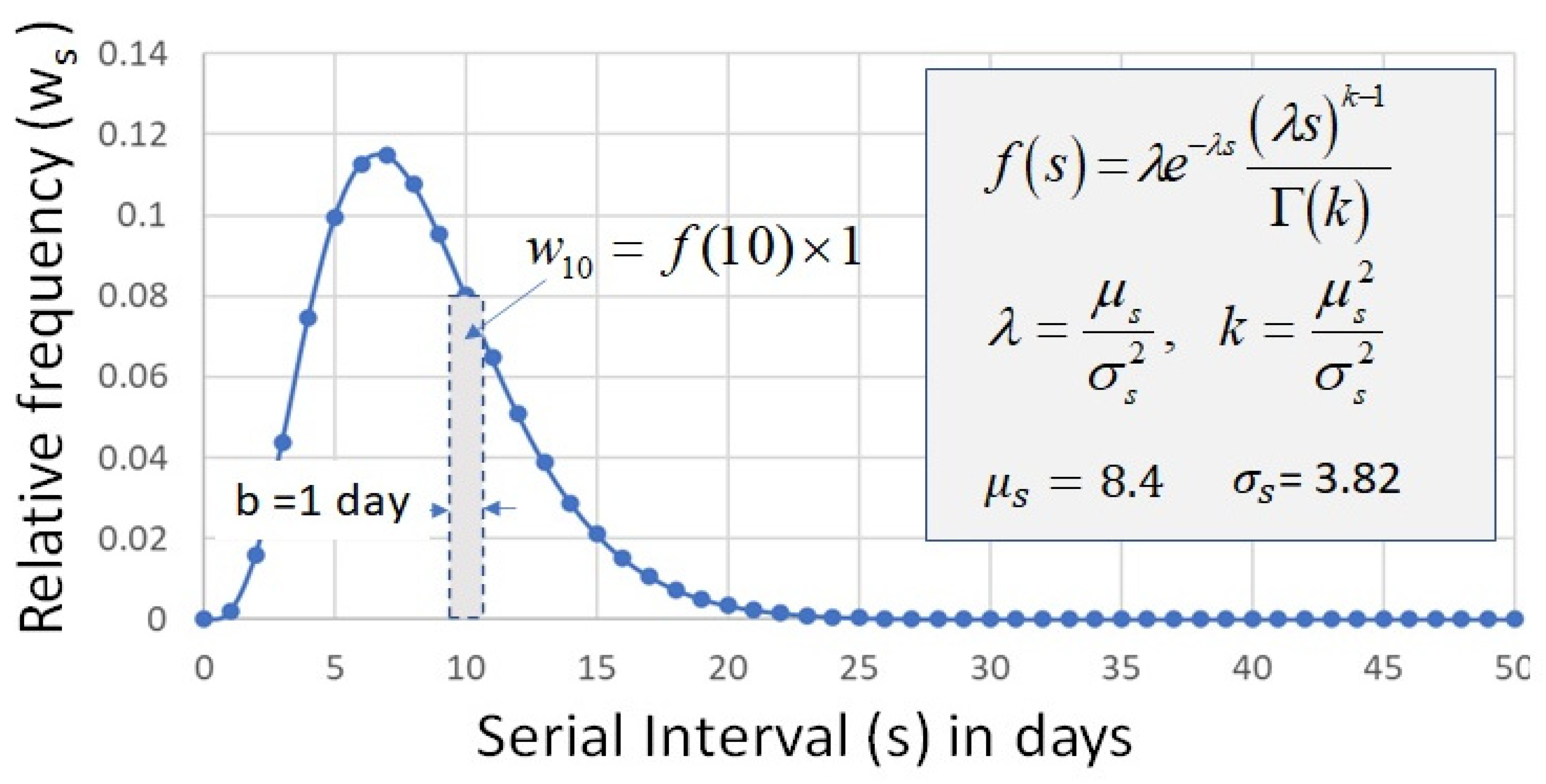
3.3. Serial Interval
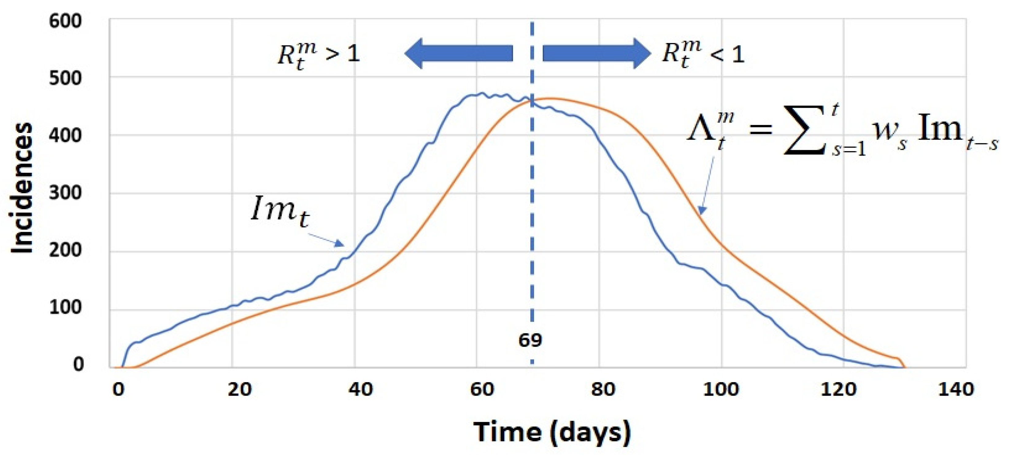
3.4. The Contagion Model
- (a)
- Keeping with the original dependency on t and s:
- (b)
- Declaring as independent of s, and keeping the dependency on t:
3.5. Frequentist Framework
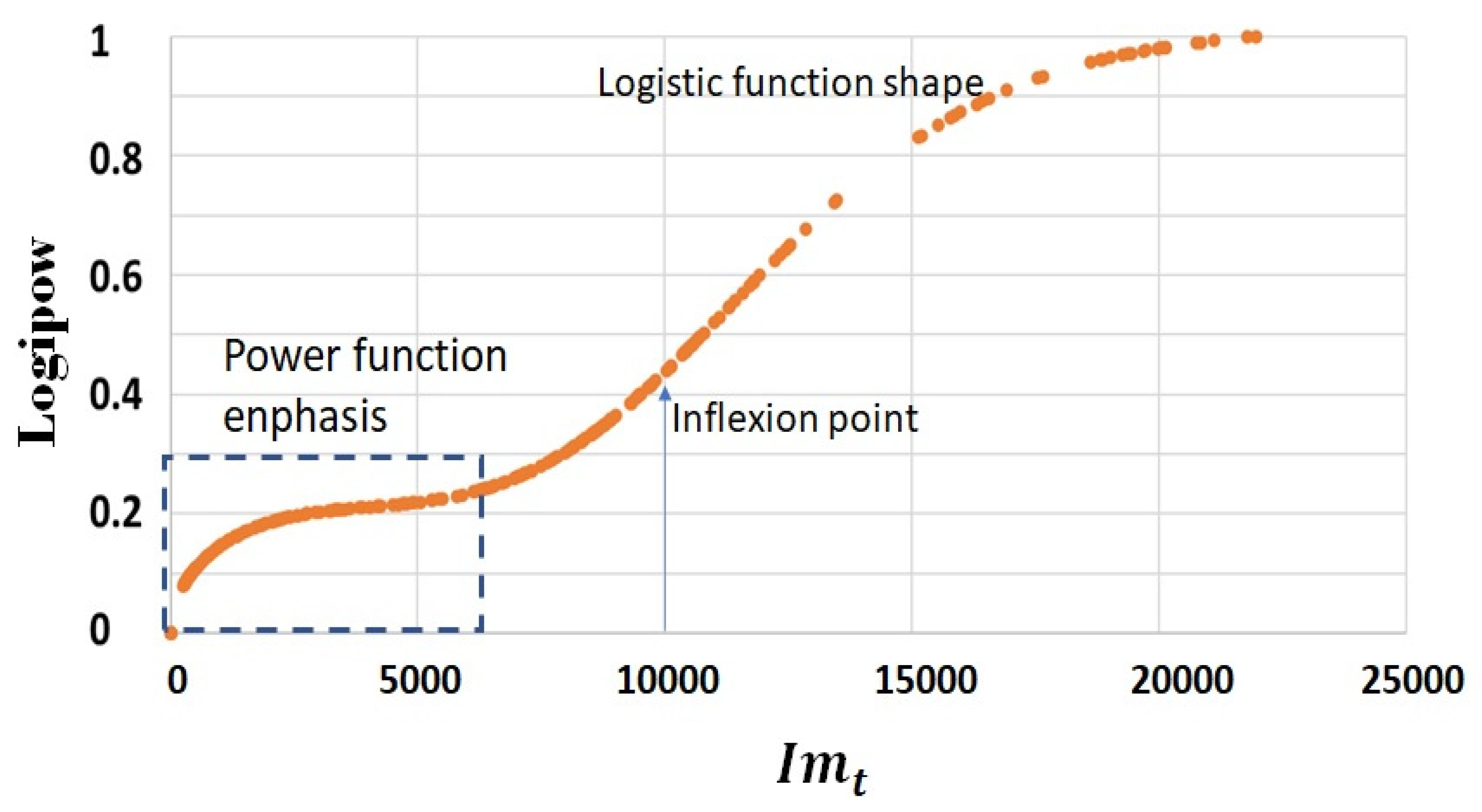
3.6. The Probability Density Function of
3.7. The Confidence Interval of
- 1.
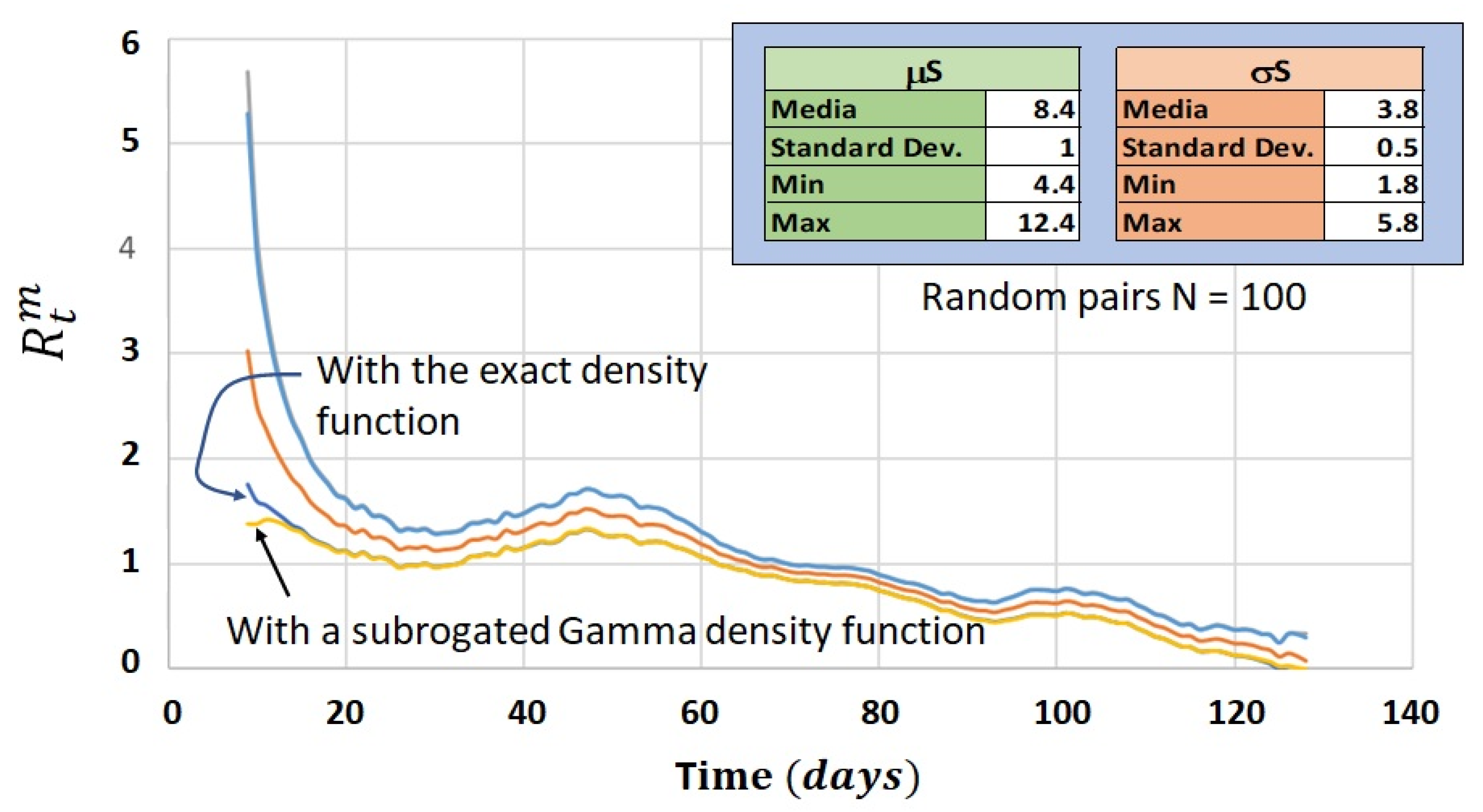
- Generate N random pairs .
- 2.
- Calculate the weights for each pair j.
- 3.
- Calculate the denominator for each pair j.Apply each pair in the calculation of :
- 4.
- Calculate the values of the means and standard deviations corresponding to each pair:
- 5.
- Calculate the general mean of all means :
- 6.
- Calculate the general standard deviation by using the following formula:
- 7.
- Given the mean (31), the standard deviation (32), and a significance level α, assuming a Gamma distribution, calculate the lower and upper limits of the confidence interval for the population mean of , for each observation instant t.
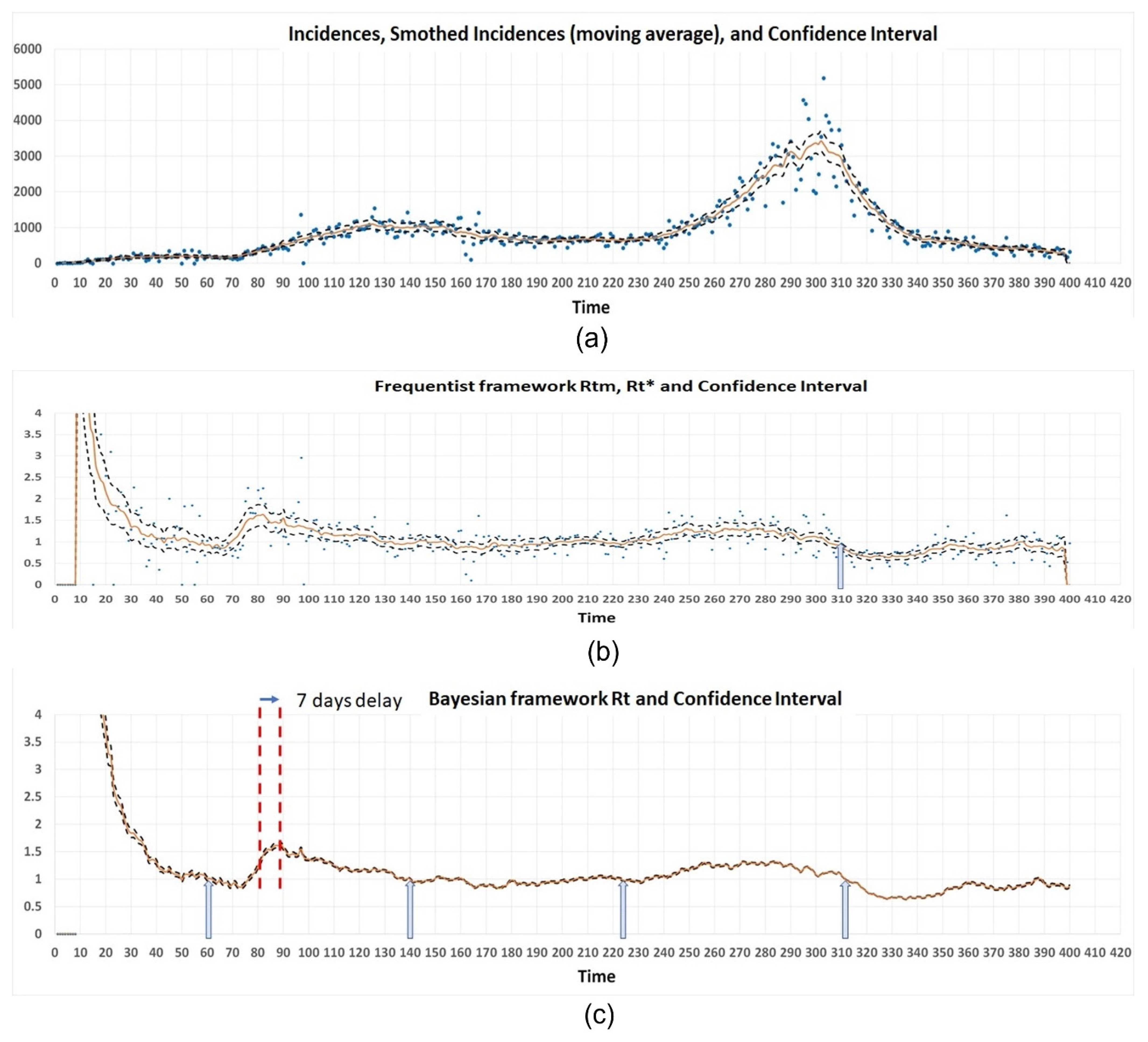
4. Results
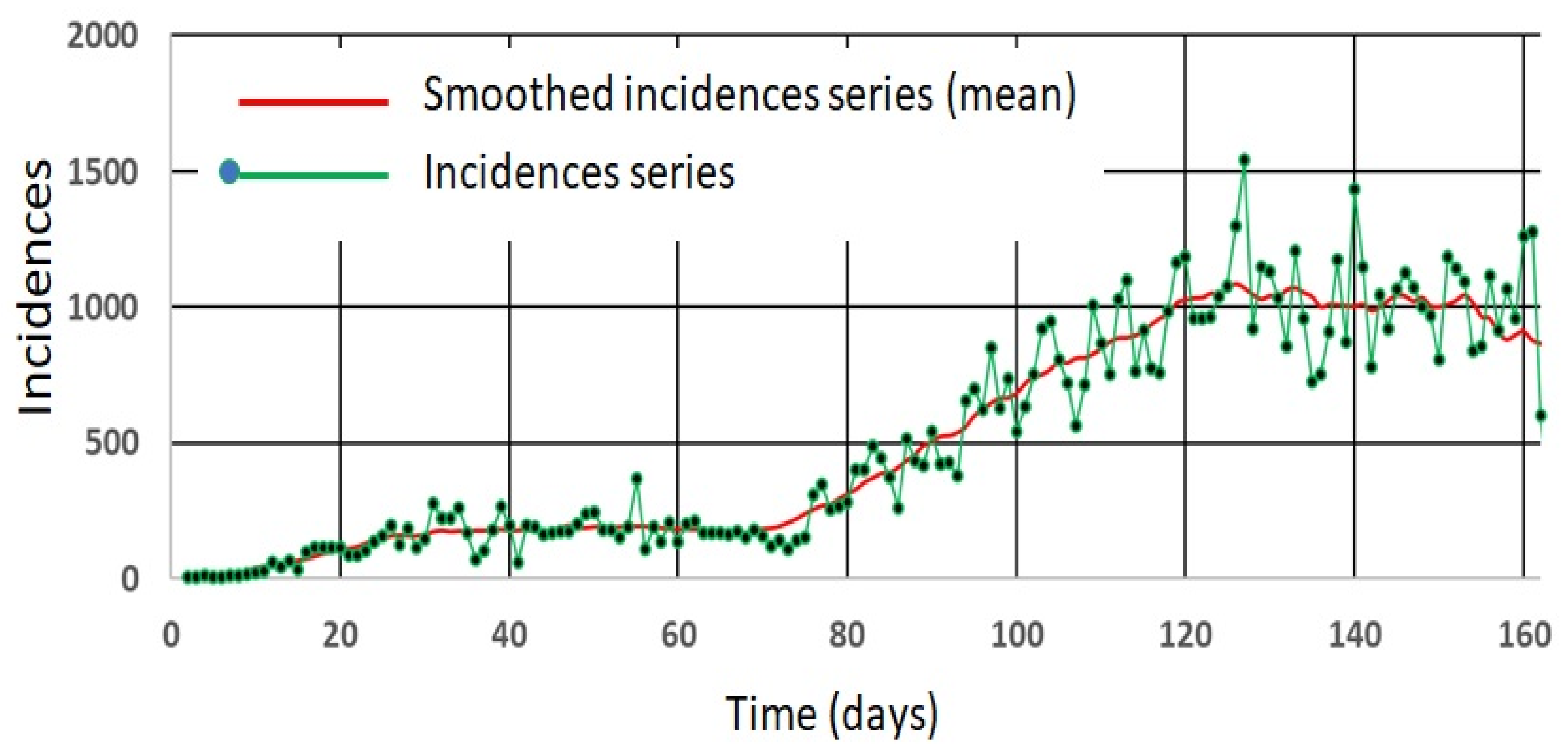
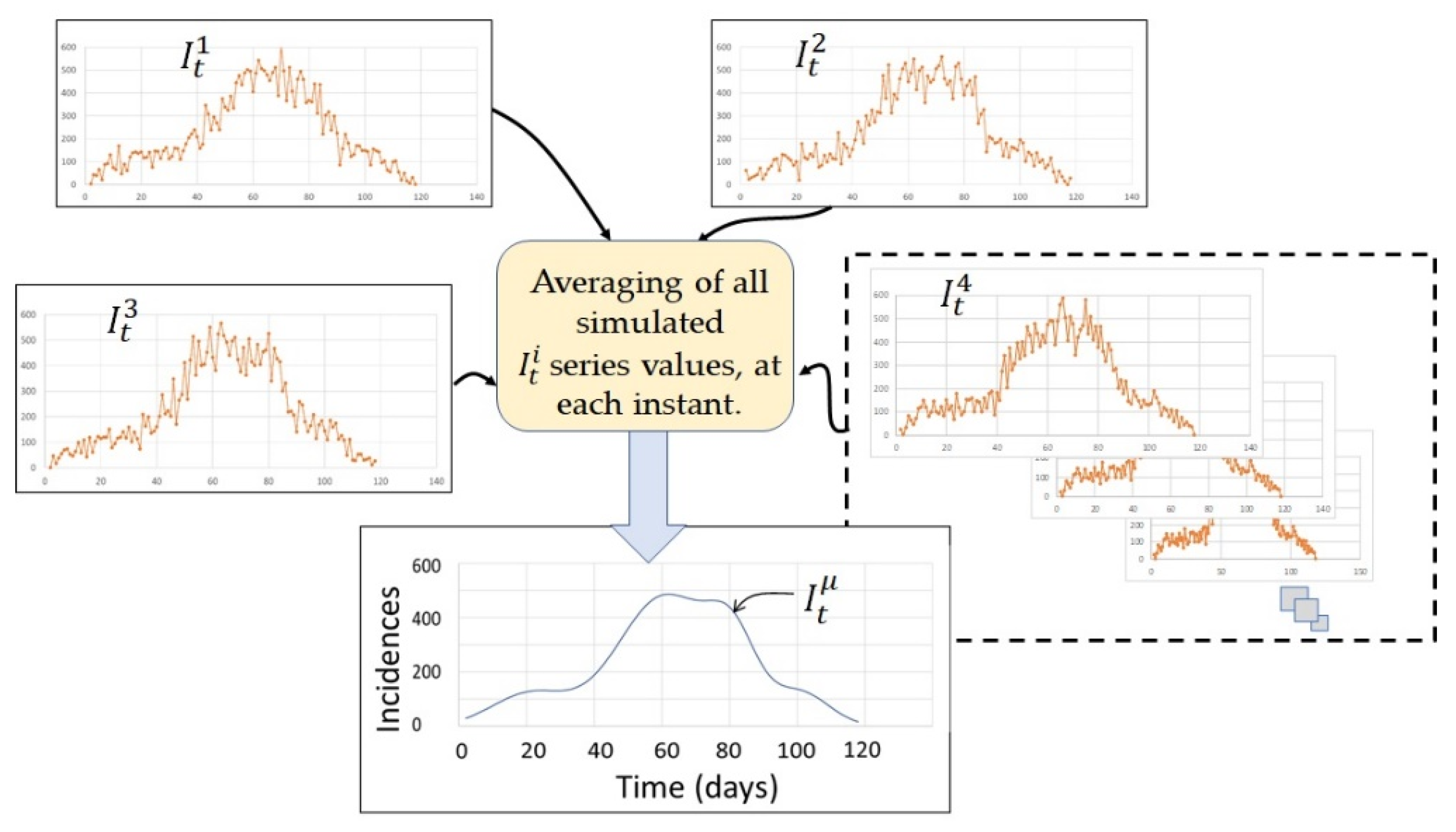
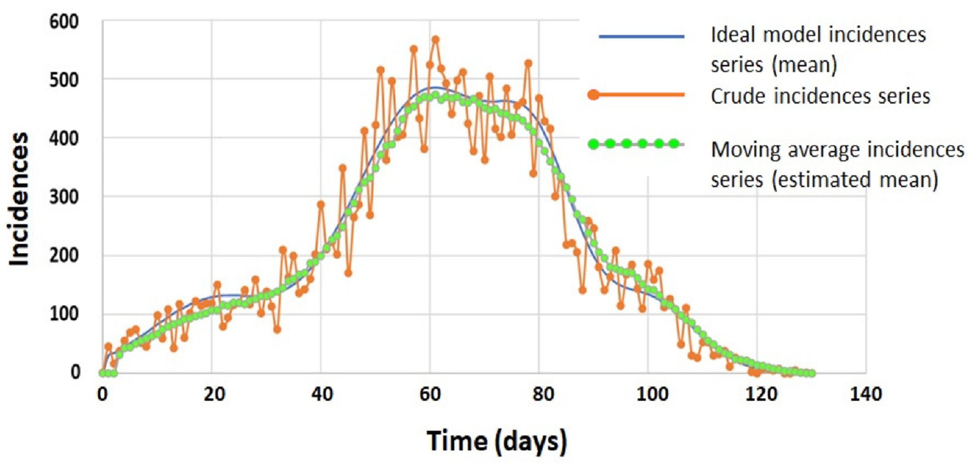
4.1. Simulated Incidence Data Series
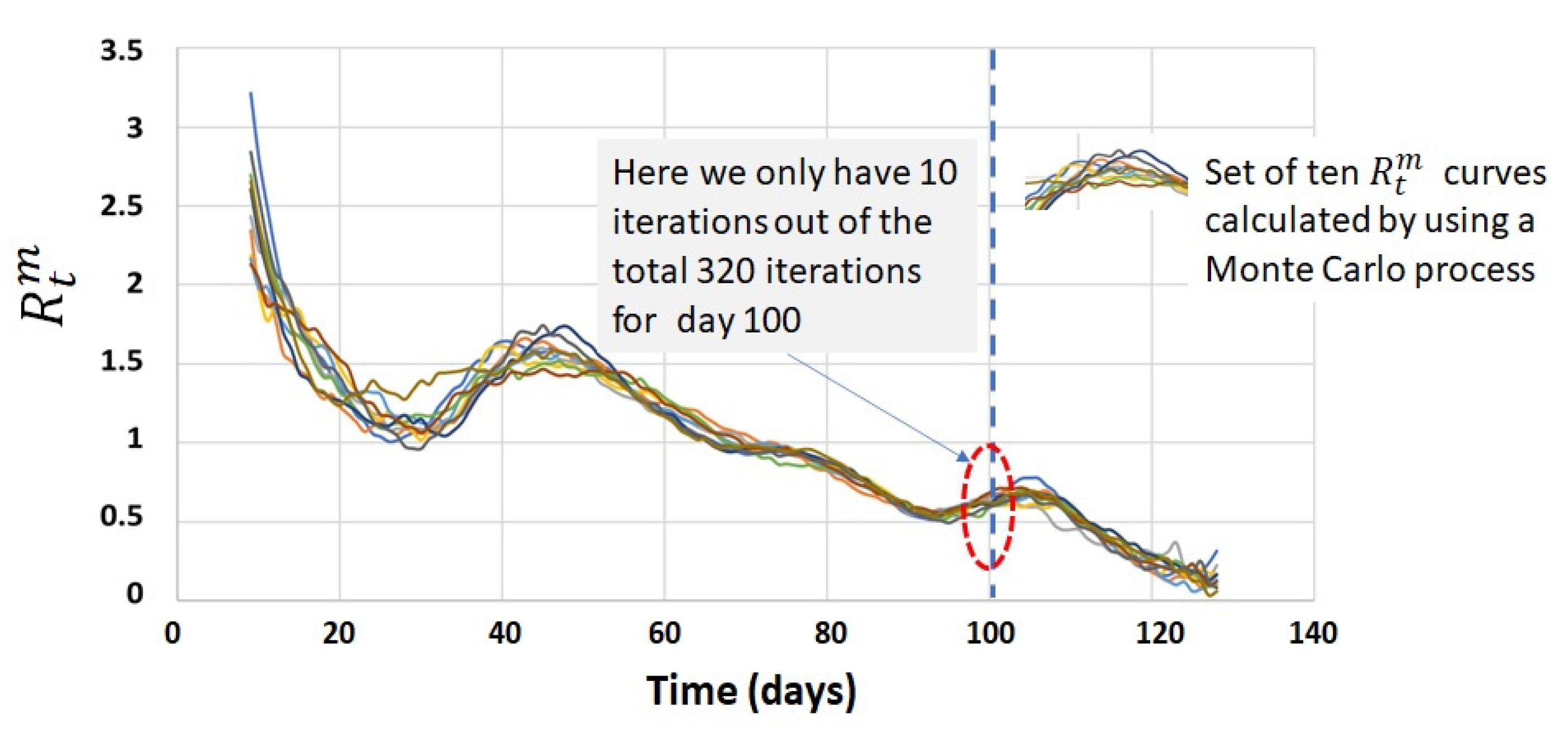
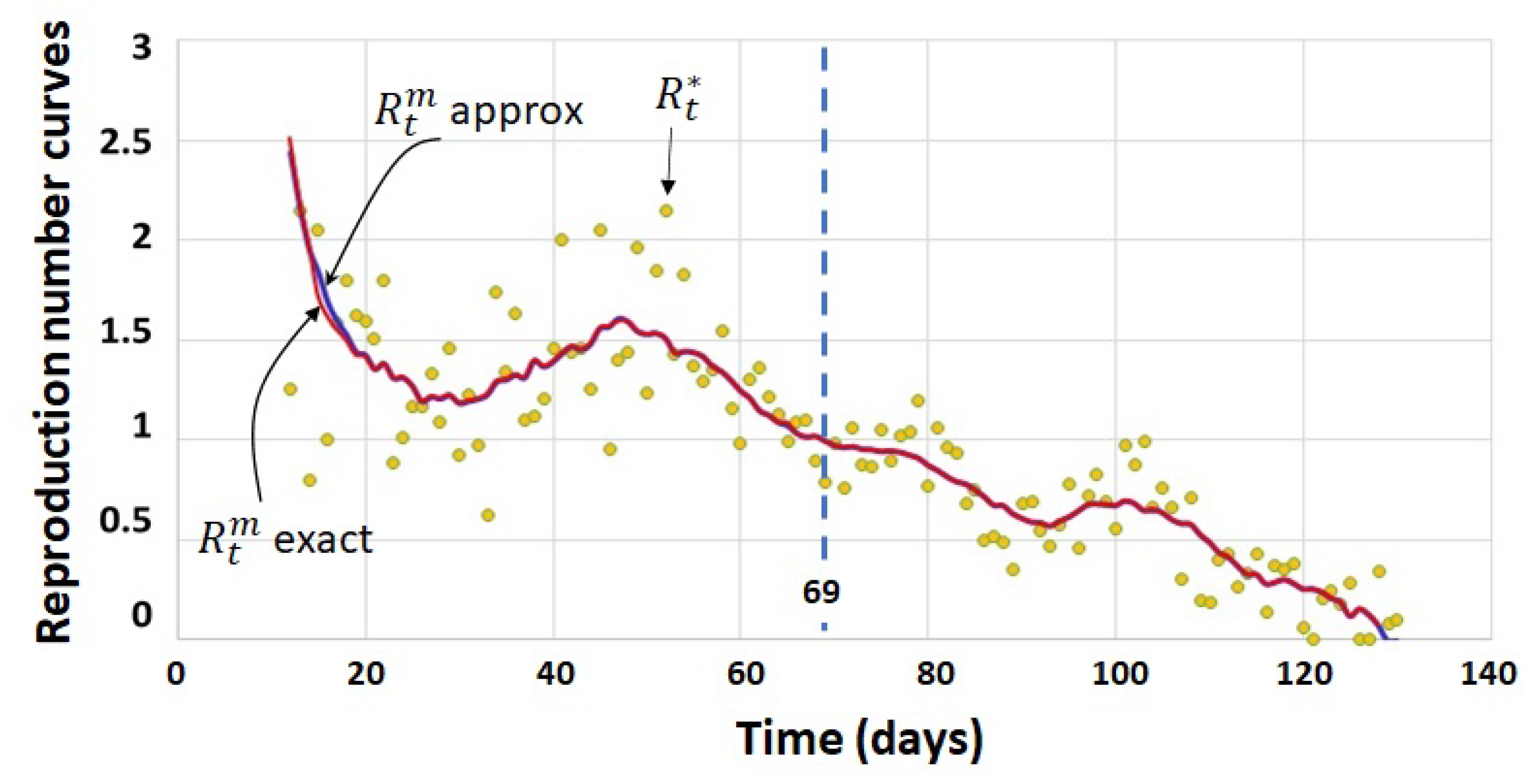
4.2. Process Calculation of
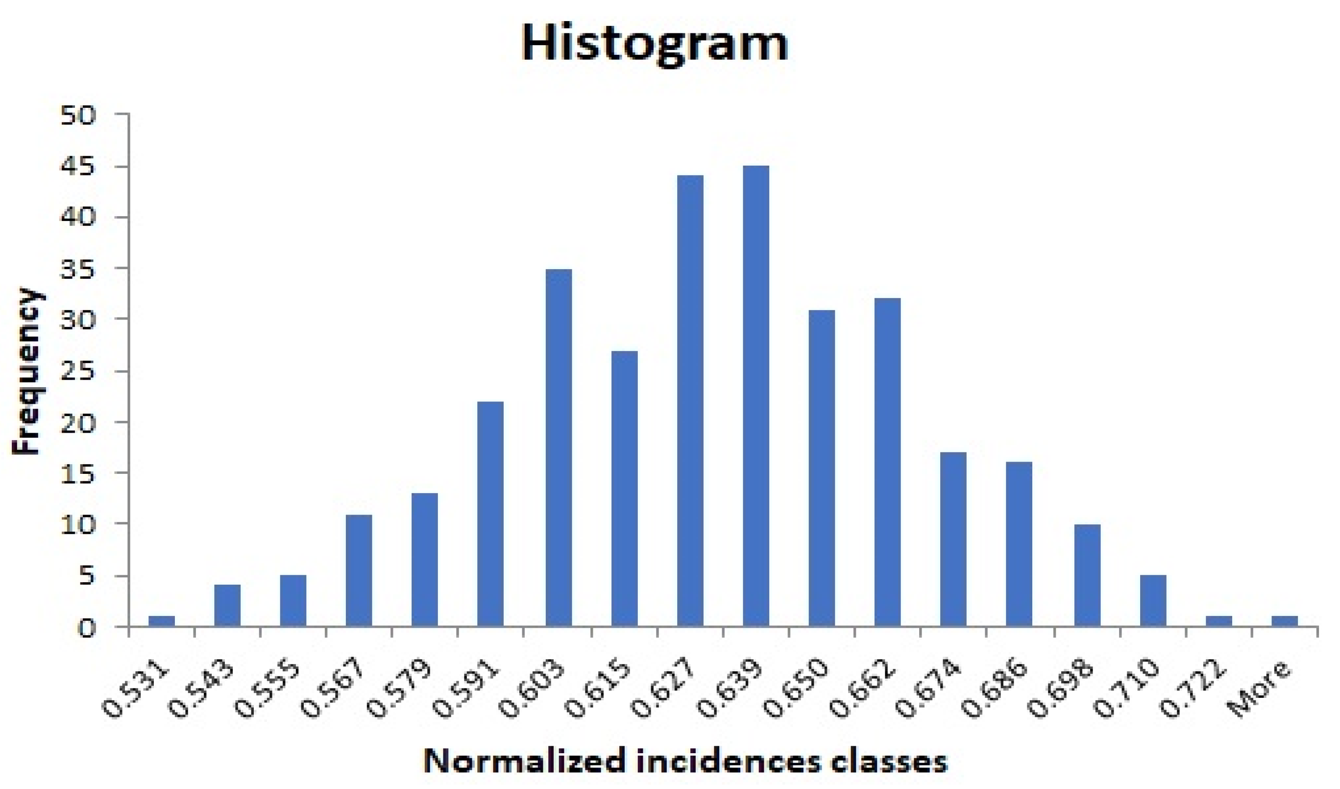
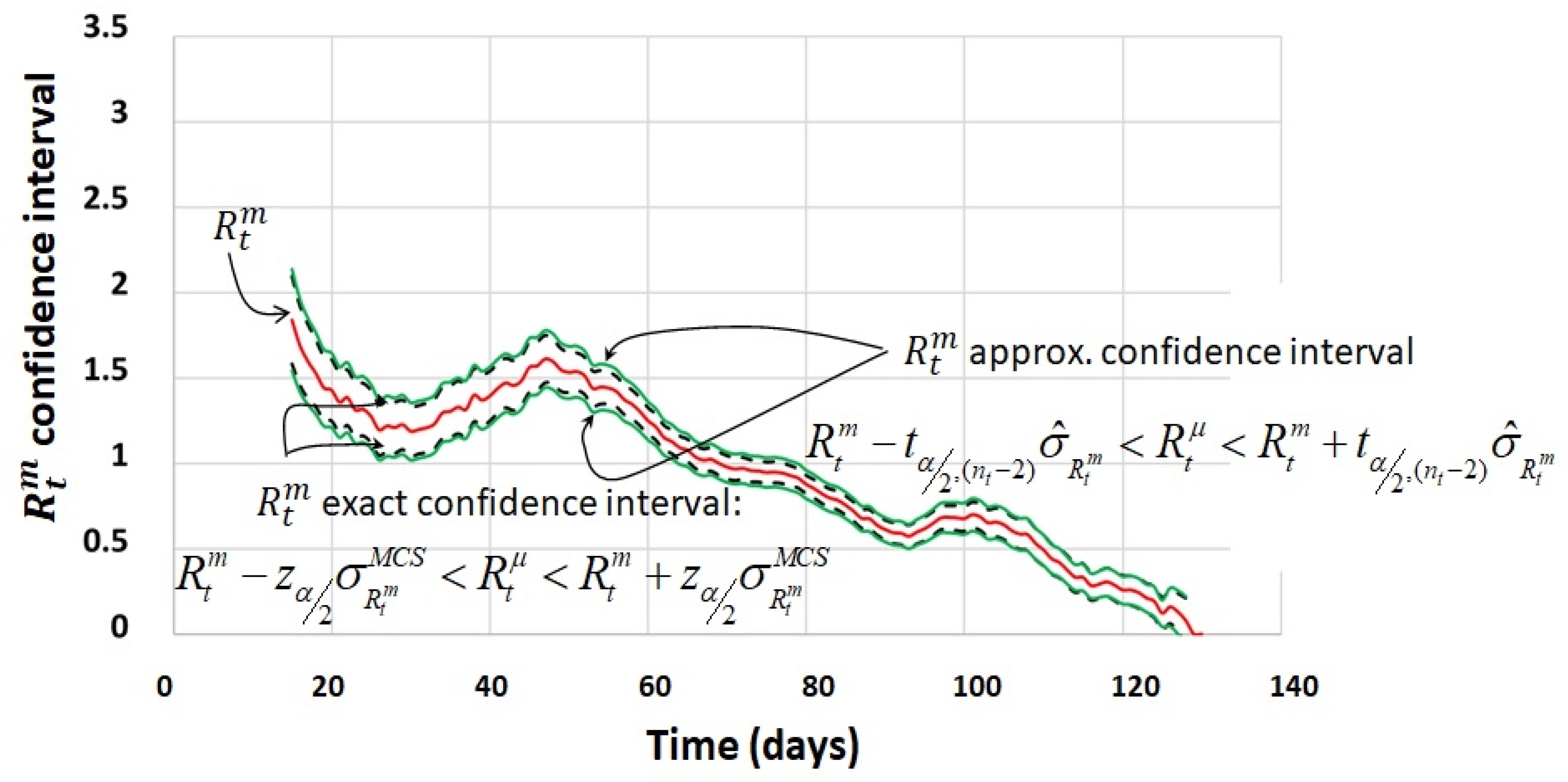
4.3. Process Calculation of the Confidence Interval
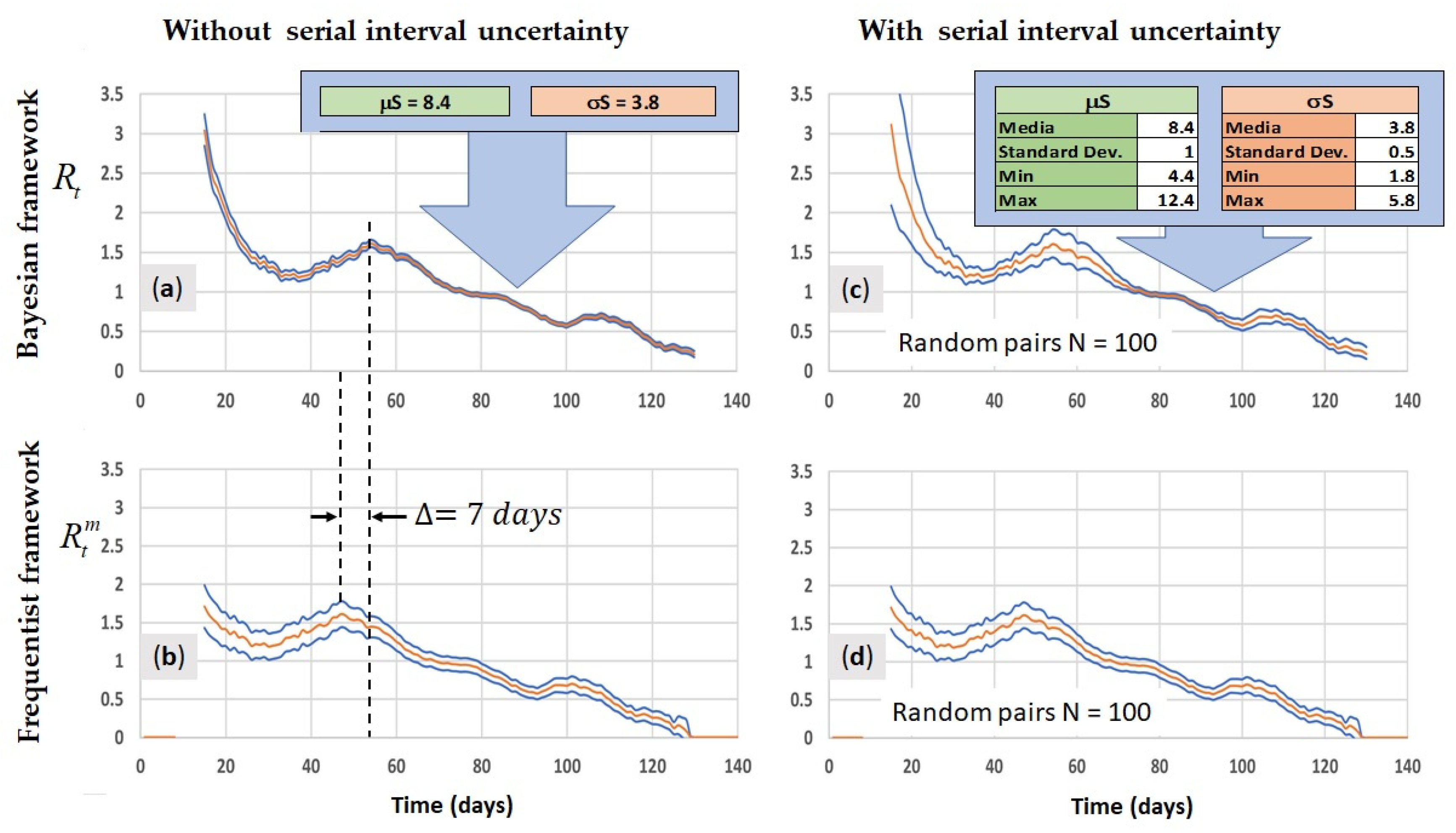
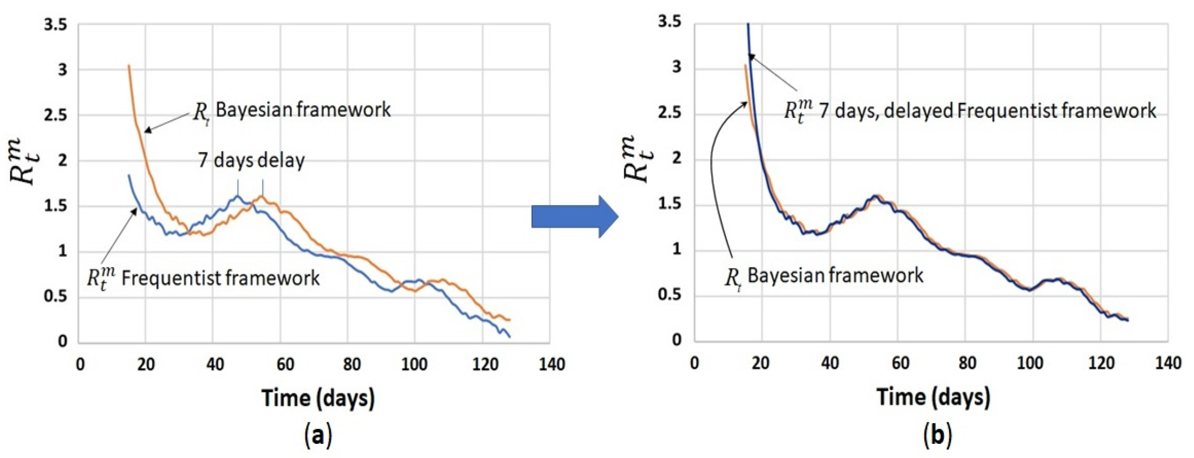
4.4. Comparison between Bayesian Method and Frequentist Method for Calculation of the Instantaneous Reproduction Number ( vs. )
4.5. A Real Case Application: Pandemic COVID-19 in Panama
4.6. Computational Aspects
5. Conclusions
Author Contributions
Funding
Institutional Review Board Statement
Informed Consent Statement
Data Availability Statement
Conflicts of Interest
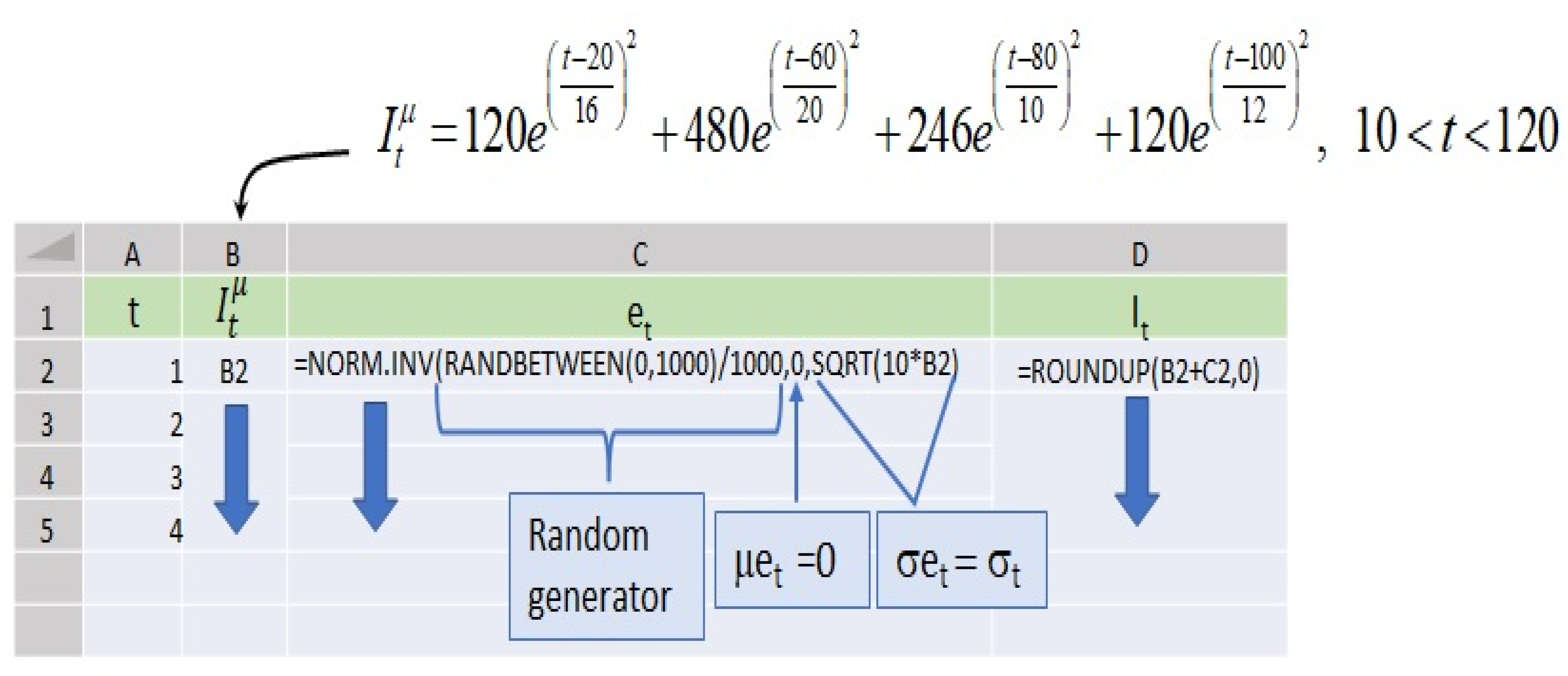
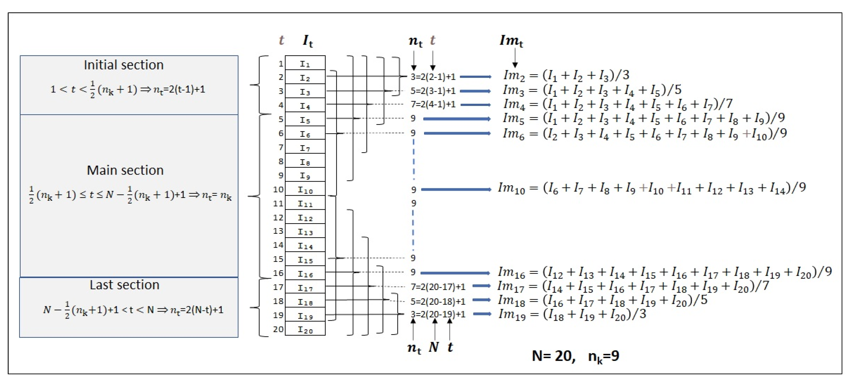
Appendix A. Modeling Incidence Series with Normal Parameters, Means, and the Standard Deviations

- Randomness of sign test (applied to ) should be passed.
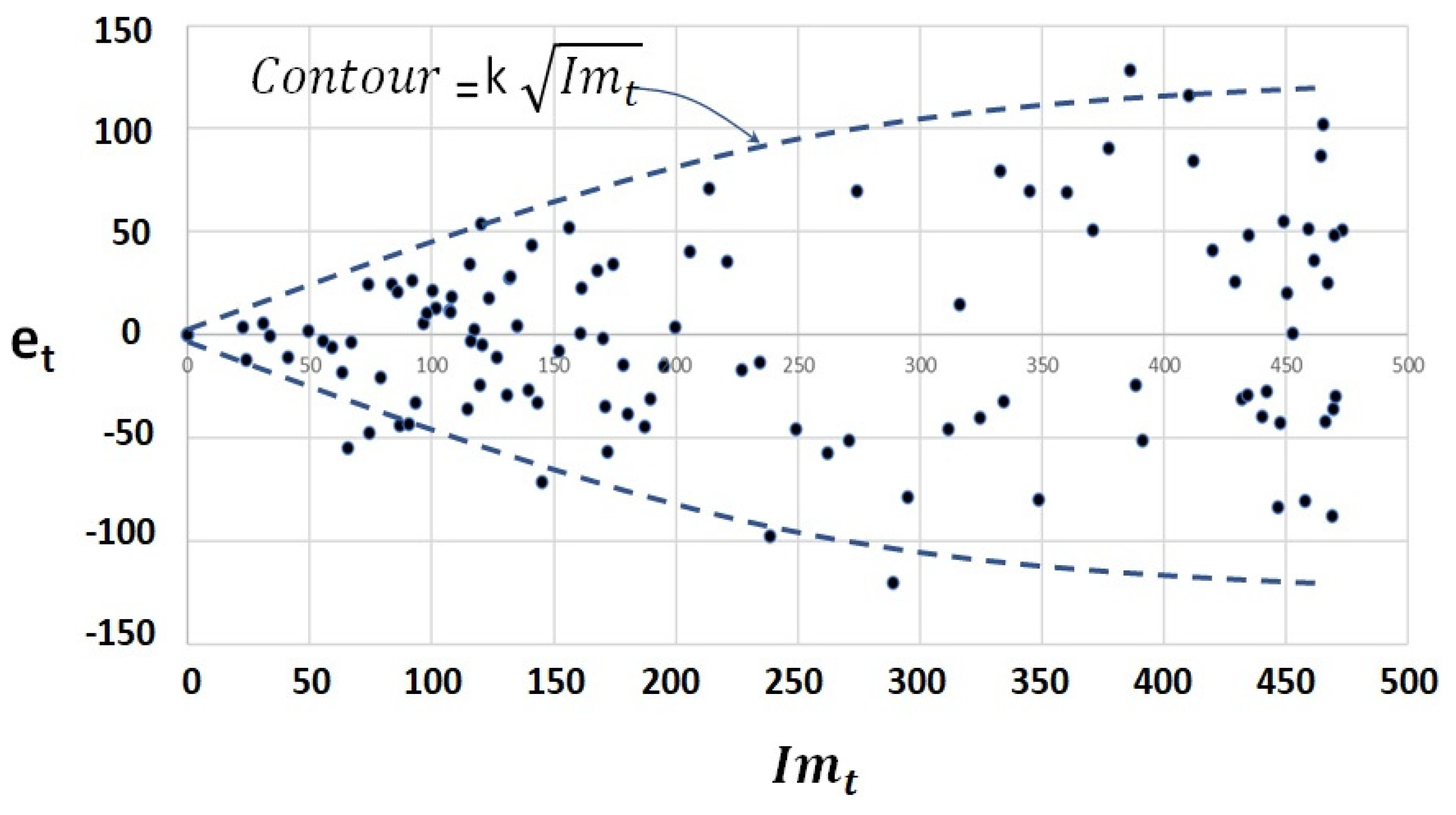
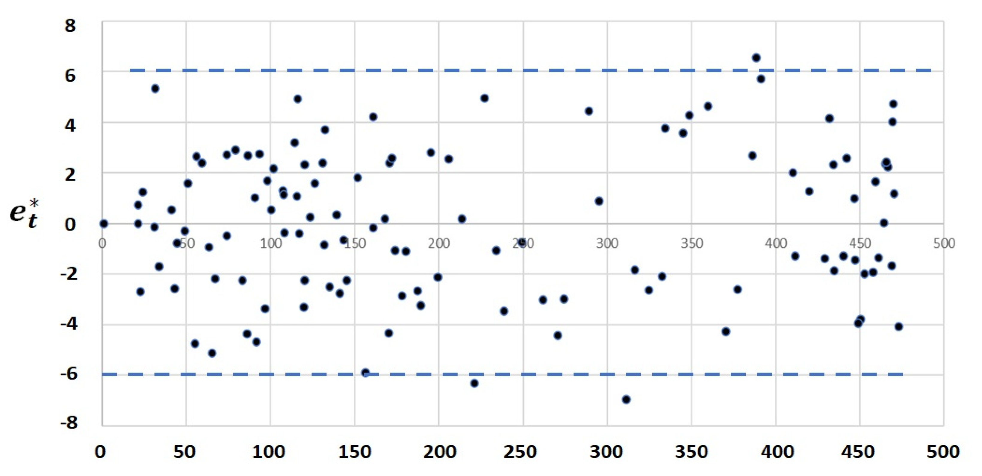
- Normality test (applied to the transformed error , below defined) should be passed.
- Histogram plot (applied to the transformed error ) should look like a normal pattern.
- Superimposed graphs of and , where the curve should “navigate” through the , revealing no aleatory patterns (for example, week periodicity).


- 1.
- Assuming that is constant within time intervals: For fixed counting process within the time intervals.
- 2.
- Assuming that is continually changing over time: For counting processes that we know are changing but do not know when they change.
Appendix B. The Probability Density Function of the Noisy Reproduction Number
Appendix C. Confidence Interval Calculation with Serial Interval Uncertainty
- 1.
- The values of the means and the variances are known and come from an unspecified random process.
- 2.
- The values of the row j of this matrix are random versions of the variable .
- 3.
- There is a global variable that we will call x, whose random values are obtained from the matrix and that has a population mean and variance . The corresponding probability density function is unknown.

References
- Gostic, K.M.; McGough, L.; Baskerville, E.B.; Abbott, S.; Joshi, K.; Tedijanto, C.; Kahn, R.; Niehus, R.; Hay, J.A.; De Salazar, P.M.; et al. Practical Considerations for Measuring the Effective Reproductive Number, Rt. PLoS Comput. Biol. 2020, 16, e1008409. [Google Scholar] [CrossRef]
- Avram, F.; Adenane, R.; Ketcheson, D.I. A Review of Matrix SIR Arino Epidemic Models. Mathematics 2021, 9, 1513. [Google Scholar] [CrossRef]
- Hussain, S.; Madi, E.; Khan, H.; Etemad, S.; Rezapour, S.; Sitthiwirattham, T.; Patanarapeelert, N. Investigation of the Stochastic Modeling of COVID-19 with Environmental Noise from the Analytical and Numerical Point of View. Mathematics 2021, 9, 3122. [Google Scholar] [CrossRef]
- Alonso-Quesada, S.; De la Sen, M.; Nistal, R. An SIRS Epidemic Model Supervised by a Control System for Vaccination and Treatment Actions Which Involve First-Order Dynamics and Vaccination of Newborns. Mathematics 2022, 10, 36. [Google Scholar] [CrossRef]
- Petermann, M.; Wyler, D. A Pitfall in Estimating the Effective Reproductive Number Rt for COVID-19. Swiss Med. Wkly. 2020, 150, w20307. [Google Scholar]
- Ganasegeran, K.; Ch’ng, A.S.H.; Looi, I. What Is the Estimated COVID-19 Reproduction Number and the Proportion of the Population That Needs to Be Immunized to Achieve Herd Immunity in Malaysia? A Mathematical Epidemiology Synthesis. COVID 2021, 1, 3. [Google Scholar] [CrossRef]
- Na, J.; Tibebu, H.; De Silva, V.; Kondoz, A. Probabilistic Approximation of Effective Reproduction Number of COVID-19 Using Daily Death Statistics. Chaos Solitons Fractals 2020, 140, 110181. [Google Scholar] [CrossRef] [PubMed]
- Knight, J.; Mishra, S. Estimating Effective Reproduction Number Using Generation Time versus Serial Interval, with Application to Covid-19 in the Greater Toronto Area, Canada. Infect. Dis Model. 2020, 5, 889–896. [Google Scholar] [CrossRef] [PubMed]
- Bacaër, N. A Short History of Mathematical Population Dynamics; Springer: Berlin/Heidelberg, Germany, 2011. [Google Scholar]
- Kermack, W.O.; McKendrick, A.G. A Contribution to the Mathematical Theory of Epidemics. Proc. R Soc. London Ser. A Contain. Pap. A Math. Phys. Character 1927, 115, 700–721. [Google Scholar] [CrossRef] [Green Version]
- Peterson, J.D.; Adhikari, R. Efficient and Flexible Methods for Time since Infection Models. arXiv 2019, arXiv:2010.10955. [Google Scholar] [CrossRef] [PubMed]
- Fraser, C. Estimating Individual and Household Reproduction Numbers in an Emerging Epidemic. PLoS ONE 2007, 2, e758. [Google Scholar] [CrossRef] [PubMed]
- Wallinga, J.; Teunis, T. Different Epidemic Curves for Severe Acute Respiratory Syndrome Reveal Similar Impacts of Control Measures. Am. J. Epidemiol. 2004, 160, 509–516. [Google Scholar] [CrossRef] [PubMed] [Green Version]
- Fine, P.E.M. The Interval between Successive Cases of an Infectious Disease. Am. J. Epidemiol. 2003, 158, 1039–1047. [Google Scholar] [CrossRef] [PubMed] [Green Version]
- Svensson, M. A Note on Generation Times in Epidemic Models. Math. Biosci. 2007, 208, 300–311. [Google Scholar] [CrossRef] [PubMed]
- Cori, A.; Ferguson, N.M.; Fraser, C.; Cauchemez, S. Practice of Epidemiology/A New Framework and Software to Estimate Time-Varying Reproduction Numbers during Epidemics. Am. J. Epidemiol. 2013, 178, 1505–1512. [Google Scholar] [CrossRef] [PubMed] [Green Version]
- Thompson, R.; Stockwind, J.; Van Gaalene, R.; Polonsky, J.; Kamvarg, Z.; Demarsh, P.; Dahlqwist, E.; Lij, S.; Miguelk, E.; Jombartg, T.; et al. Improved Inference of Time-Varying Reproduction Numbers during Infectious Disease Outbreaks. Epidemics 2019, 29, 100356. [Google Scholar] [CrossRef] [PubMed]
- Cabras, S. A Bayesian-Deep Learning Model for Estimating Covid-19 Evolution in Spain. Mathematics 2021, 9, 2921. [Google Scholar] [CrossRef]
- Xu, J.; Tang, Y. Mathematics Bayesian Framework for Multi-Wave COVID-19 Epidemic Analysis Using Empirical Vaccination Data Framework for Multi-Wave. Mathematics 2022, 10, 22. [Google Scholar] [CrossRef]
- Zhao, S.; Cao, P.; Gao, D.; Zhuang, Z.; Cai, Y.; Ran, J.; Chong, M.K.C.; Wang, K.; Lou, Y.; Wang, W.; et al. Serial Interval in Determining the Estimation of Reproduction Number of the Novel Coronavirus Disease (COVID-19) during the Early Outbreak. J. Travel Med. 2020, 27, 1–3. [Google Scholar] [CrossRef]
- Wheelwright, S.; Makridakis, S.; Hyndman, R. Forecasting: Methods and Applications; John Wiley & Sons: Hoboken, NJ, USA, 1998. [Google Scholar]
- Montgomery, D. Introduction to Statistical Quality Control, 4th ed.; John Wiley & Sons, Inc.: Hoboken, NJ, USA, 2001. [Google Scholar]
- Larsen, R.; Marx, M. An Introduction to Mathematical Statistics, 5th ed.; Prentice Hall/Pearson: Hoboken, NJ, USA, 2012. [Google Scholar]


| Year | Author | Subject | Deterministic (O)/Stochastic (X) | Stochastic Framework | Variability Considered | Method for Confidence Interval Calculation | Potential to Control the Sanitary and Governmental Processes of the Epidemics from the Perspective of Statistical Control Process |
|---|---|---|---|---|---|---|---|
| 1927 | Kermack & MacKendrick | SIR | O | ||||
| 2003 | Fine | Transmission interval | X | ||||
| 2004 | Wallinga & Teunis | Effective reproduction (case) | X | Bayesian | Poisson | Not declared | No |
| 2007 | Svensson | Generation time and serial interval | X | ||||
| 2007 | Fraser | Instantaneous reproduction number and case (cohort) reproduction number | X | Frequentist | All | Experimental (Bootstrapping) | Could be difficult with bootstrapping techniques |
| 2013 | Cori et al. | Instantaneous reproduction number | X | Bayesian | Poisson | Analytically (Gamma distribution) | No |
| 2019 | Thompson et al. | Instantaneous reproduction number | X | Bayesian | Poisson | Bayesian method (Credible interval) | No |
| 2020 | Peterson & Adhikari | Time since infection models | O | ||||
| 2020 | Zhao et al. | Serial interval | X | ||||
| 2021 | Cortés-Carvajal, P.D.; Cubilla Montilla, M.; González-Cortés, D.R. | Instantaneous reproduction number | X | Frequentist | All | Analytically (Normal distribution, using the central limit theorem) | Yes |
| iterations |  | |||||||||
| Day | Rtm 314 | Rtm 315 | Rtm 316 | Rtm 317 | Rtm 318 | Rtm 319 | Rtm 320 | SD MCS |  | |
| 11 | 2.17001 | 2.26392 | 2.47387 | 1.97609 | 2.00207 | 2.25481 | 2.07686 | 0.542613 | Standard | |
| 12 | 2.06127 | 2.11066 | 2.41122 | 1.87018 | 1.79859 | 2.13629 | 1.93210 | 0.589714 | deviation | |
| 13 | 1.91099 | 2.06799 | 2.32853 | 1.74570 | 1.75767 | 2.05797 | 1.89229 | 0.640457 | ||
| 14 | 1.89529 | 1.86216 | 2.25943 | 1.59517 | 1.69615 | 1.94120 | 1.83866 | 0.69466 | ||
| 15 | 1.85282 | 1.79917 | 2.14870 | 1.47665 | 1.70210 | 1.86042 | 1.77167 | 0.751537 | ||
| 16 | 1.86321 | 1.68052 | 1.92846 | 1.42572 | 1.68435 | 1.76157 | 1.60419 | 0.808612 | ||
| 17 | 1.75908 | 1.62979 | 1.83304 | 1.35254 | 1.57679 | 1.67131 | 1.57936 | 0.866715 | ||
| 18 | 1.69122 | 1.59028 | 1.75054 | 1.38187 | 1.50763 | 1.55256 | 1.51021 | 0.924422 | ||
| 19 | 1.59302 | 1.53044 | 1.68361 | 1.35205 | 1.43605 | 1.54926 | 1.40478 | 0.982537 | ||
| 20 | 1.53617 | 1.46193 | 1.61977 | 1.28381 | 1.42267 | 1.43287 | 1.31839 | 1.040908 | ||
| 21 | 1.52046 | 1.38184 | 1.61057 | 1.25251 | 1.45462 | 1.36895 | 1.22546 | 1.099110 | ||
| 22 | 1.45647 | 1.30902 | 1.54020 | 1.23288 | 1.42035 | 1.35385 | 1.13442 | 1.157020 | ||
Publisher’s Note: MDPI stays neutral with regard to jurisdictional claims in published maps and institutional affiliations. |
© 2022 by the authors. Licensee MDPI, Basel, Switzerland. This article is an open access article distributed under the terms and conditions of the Creative Commons Attribution (CC BY) license (https://creativecommons.org/licenses/by/4.0/).
Share and Cite
Cortés-Carvajal, P.D.; Cubilla-Montilla, M.; González-Cortés, D.R. Estimation of the Instantaneous Reproduction Number and Its Confidence Interval for Modeling the COVID-19 Pandemic. Mathematics 2022, 10, 287. https://0-doi-org.brum.beds.ac.uk/10.3390/math10020287
Cortés-Carvajal PD, Cubilla-Montilla M, González-Cortés DR. Estimation of the Instantaneous Reproduction Number and Its Confidence Interval for Modeling the COVID-19 Pandemic. Mathematics. 2022; 10(2):287. https://0-doi-org.brum.beds.ac.uk/10.3390/math10020287
Chicago/Turabian StyleCortés-Carvajal, Publio Darío, Mitzi Cubilla-Montilla, and David Ricardo González-Cortés. 2022. "Estimation of the Instantaneous Reproduction Number and Its Confidence Interval for Modeling the COVID-19 Pandemic" Mathematics 10, no. 2: 287. https://0-doi-org.brum.beds.ac.uk/10.3390/math10020287