Synchronization of Nonlinear Complex Spatiotemporal Networks Based on PIDEs with Multiple Time Delays: A P-sD Method

Abstract

This paper studies the synchronization control of nonlinear multiple time-delayed complex spatiotemporal networks (MTDCSNs) based on partial integro-differential equations. Firstly, dealing with an MTDCSN with time-invariant delays, P-sD control is employed and the synchronization criteria are obtained in terms of LMIs. Secondly, this control method is further used in an MTDCSN with time-varying delays. An example illustrates the effectiveness of the proposed methods.

1. Introduction

As a typical collective behavior in nature, the synchronization of complex networks has attracted a great deal of attention during the last few decades [1,2,3]. It has been widely applied to engineering fields, such as secure communication [4,5], deception attacks [6,7,8], the design of pseudorandom number generators [9], and image encryption [10].

In fact, many phenomena rely not only on time but also on space [11,12,13]. As a result, many researchers have studied complex spatiotemporal networks (CSNs), owing to many phenomena relating not only to time but also to space. Kanakov et al. studied the cluster synchronization of the CSNs of oscillatory and excitable Luo–Rudy cells [14]. Kakmeni and Baptista proposed synchronization and information transmission in CSNs under a substrate Remoissenet–Peyrard potential [15]. Rybalova et al. investigated complete synchronization under the condition of spatio-temporal chaos with the Henon map and Lozi map [16]. Yang et al. studied the guaranteed cost boundary control of nonlinear CSNs with a community structure [17] and the boundary control of CSNs modeled by partial differential equations–ordinary differential Equations (PDE-ODEs) [18].

Owing to the extensive existence of time delays, it is important to research time-delayed networks [19,20,21,22]. Yao et al. studied the passive stability and synchronization of switching CSNs with time delays in terms of appropriate algebraic inequalities [23,24]. Zhou et al. proposed two methods—matrix invertibility and an adaptive law—for the topology identification and finite-time topology identification of time-delayed complex spatiotemporal networks (TDCSNs) [25,26]. Sheng et al. studied the exponential synchronization of TDCSNs with Dirichlet boundary conditions and hybrid time delays via impulsive control [27]. Lu et al. studied generalized sampled-data intermittent control for the exponential synchronization of TDCSNs [28]. Yang et al. proposed the synchronization of nonlinear complex spatio-temporal networks with multiple time-invariant delays and multiple time-varying delays [29]. Zhang et al. proposed fuzzy time sampled-data control and fuzzy time–space sampled-data control for the synchronization of T–S fuzzy TDCSNs with additive time-varying delays [30].

On the whole, most of the mentioned literature assumes that nodes are modeled by partial differential equations, PDEs, or PDE-ODEs. Few studies consider models based on partial integro-differential Equations (PIDEs). PIDEs have been applied to spread and traveling waves [31], pricing models [32], biology [33], pattern formation [34], secure communication [5], and medical science [35]. Many dynamical behaviors of PIDEs have been studied [36,37,38]. However, there are still some technical difficulties in the synchronization of multiple time-delayed TDCSNs based on PIDEs, such as communication among nodes and controller design, which is the motivation for this paper.

Notations: I means an identity matrix with proper order; $P<0$ is a negative definite matrix, while $P>0$ is positive definite; `*’ is an ellipsis of transpose blocks in symmetric matrices.

2. Problem Formulation

This paper studies a class of nonlinear MTDCSNs based on PIDEs:

$$\begin{array}{ccc}\hfill \frac{\partial y_i(\zeta ,t)}{\partial t}& =& {\Theta }_1\frac{{\partial }^2{y}_i(\zeta ,t)}{\partial {\zeta }^2}+{\Theta }_2\frac{\partial y_i(\zeta ,t)}{\partial \zeta }+A{y}_i(\zeta ,t-{\tau }_1\left(t\right))+f\left(y_i(\zeta ,t-{\tau }_2\left(t\right))\right)\hfill \\ \hfill & & +B{\int }_0^{\zeta }{y}_i(z,t-{\tau }_3\left(t\right))dz+c\sum _{j=1}^N{h}_{ij}\Gamma y_j(\zeta ,t-{\tau }_4\left(t\right))+u_i(\zeta ,t),\hfill \\ \hfill \frac{\partial y_i(0,t)}{\partial \zeta }& =& 0,\frac{\partial y_i(L,t)}{\partial \zeta }=0,\hfill \\ \hfill y_i(\zeta ,t)& =& y_i^0(\zeta ,t),(\zeta ,t)\in [0,L]\times [-\tau ,0],\hfill \end{array}$$

(1)

where $(\zeta ,t)\in [0,L]\times [0,\infty )$. Here, $y_i(\zeta ,t),u_i(\zeta ,t)\in {\mathbb{R}}^n$ are the respective state and control inputs, $i\in \{1,2,\cdots ,N\}$. ${\Theta }_1\in {\mathbb{R}}^{n\times n}$ is the diffusion coefficient matrix. ${\Theta }_2\in {\mathbb{R}}^{n\times n}$ is the convection coefficient matrix. $A\in {\mathbb{R}}^{n\times n}$ and $B\in {\mathbb{R}}^{n\times n}$ are the connection matrices. $0<\Gamma \in {\mathbb{R}}^{n\times n}$ is the inner coupling matrix. The coupling strength c is a positive real number. The coupling connection $H={\left(h_{ij}\right)}_{N\times N}$ is defined as $h_{ij}>0(i\ne j)$ if the agent j connects to i and $h_{ii}=-{\displaystyle \sum _{j\ne i}}{h}_{ij}$. $f(·)$ is a nonlinear function that varies over time and space. $0<{\tau }_1\left(t\right),{\tau }_2\left(t\right),{\tau }_3\left(t\right),{\tau }_4\left(t\right)\le \tau$, ${\dot{\tau }}_1\left(t\right)⩽{\mu }_1$, ${\dot{\tau }}_2\left(t\right)⩽{\mu }_2$, ${\dot{\tau }}_3\left(t\right)⩽{\mu }_3$, and ${\dot{\tau }}_4\left(t\right)⩽{\mu }_4$.

The isolated node is supposed to be:

$$\begin{array}{ccc}\hfill \frac{\partial s(\zeta ,t)}{\partial t}& =& {\Theta }_1\frac{{\partial }^{2}s(\zeta ,t)}{\partial {\zeta }^2}+{\Theta }_2\frac{\partial s(\zeta ,t)}{\partial \zeta }+As(\zeta ,t-{\tau }_1\left(t\right))+f\left(s(\zeta ,t-{\tau }_2\left(t\right))\right)\hfill \\ \hfill & & +B{\int }_0^{\zeta }s(z,t-{\tau }_3\left(t\right))dz,\hfill \\ \hfill \frac{\partial s(0,t)}{\partial \zeta }& =& 0,\frac{\partial s(L,t)}{\partial \zeta }=0,\hfill \\ \hfill s(\zeta ,t)& =& s^0(\zeta ,t),(\zeta ,t)\in [0,L]\times [-\tau ,0].\hfill \end{array}$$

(2)

We denote the synchronization error as ${ϵ}_i(\zeta ,t)\stackrel{\Delta }{=}{y}_i(\zeta ,t)-s(\zeta ,t)$. The P-sD controller is designed as

$$u_i(\zeta ,t)=-K_{Pi}{ϵ}_i(\zeta ,t)-K_{Di}\frac{\partial {ϵ}_i(\zeta ,t)}{\partial \zeta },$$

(3)

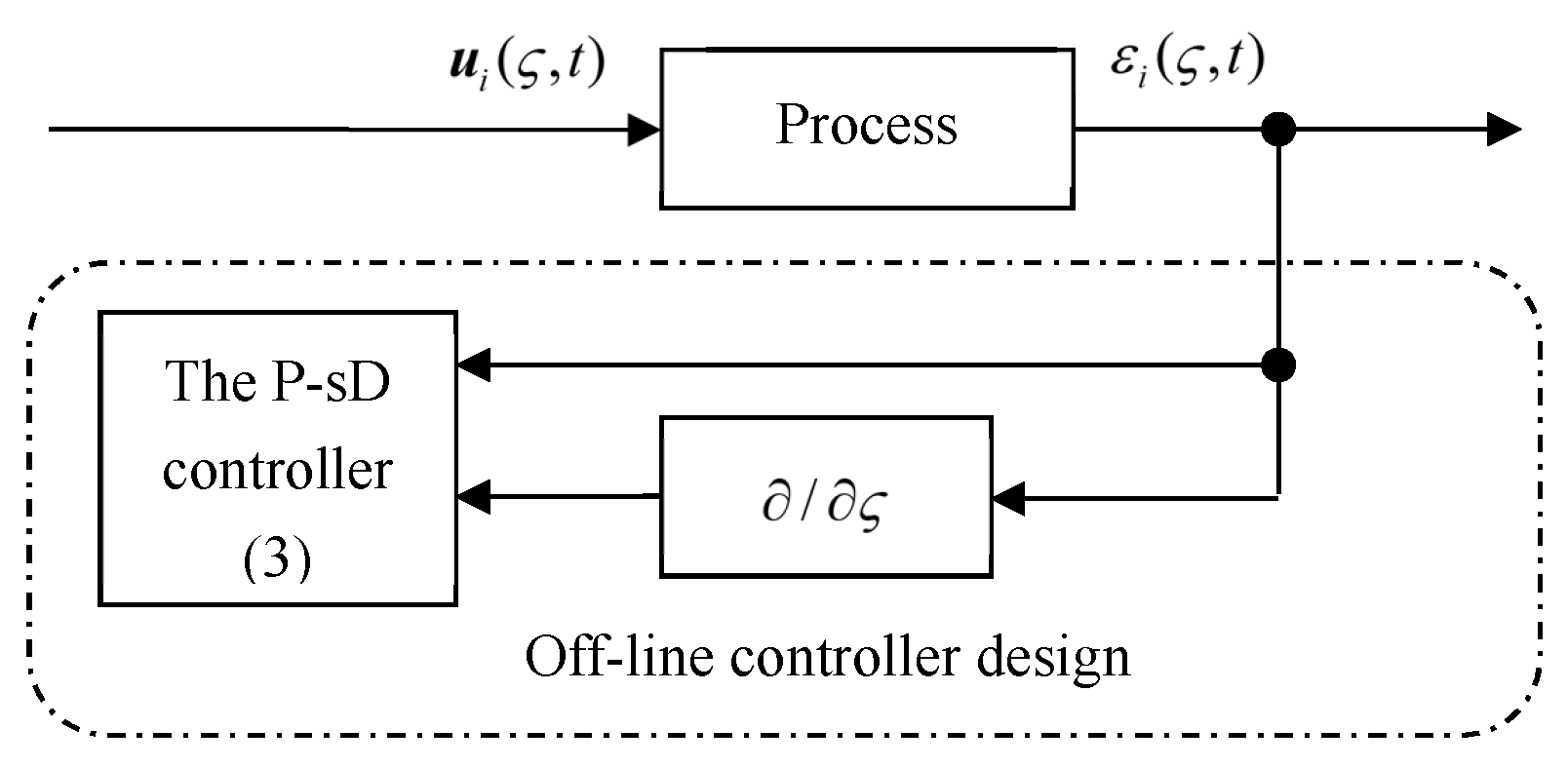
where $K_{Pi}$, $K_{Di}\in {\mathbb{R}}^{n\times n}$, $i\in \{1,2,\cdots ,N\}$, need to be determined. The controller structure in this paper is shown in Figure 1, where the notation “$\partial /\partial \zeta$” represents a first-order spatial differentiator. With (3), the error system of the MTDCSN (1) can be obtained as:

$$\begin{array}{ccc}\hfill \frac{\partial {ϵ}_i(\zeta ,t)}{\partial t}& =& {\Theta }_1\frac{{\partial }^2{ϵ}_i(\zeta ,t)}{\partial {\zeta }^2}+{\Theta }_2\frac{\partial {ϵ}_i(\zeta ,t)}{\partial \zeta }-K_{Di}\frac{\partial {ϵ}_i(\zeta ,t)}{\partial \zeta }-K_{Pi}{ϵ}_i(\zeta ,t)\hfill \\ \hfill & & +A{ϵ}_i(\zeta ,t-{\tau }_1\left(t\right))+F\left({ϵ}_i(\zeta ,t-{\tau }_2\left(t\right))\right)\hfill \\ & & +B{\int }_0^{\zeta }{ϵ}_i(s,t-{\tau }_3\left(t\right))ds+c\sum _{j=1}^N{h}_{ij}\Gamma {ϵ}_j(\zeta ,t-{\tau }_4\left(t\right)),\hfill \\ \hfill \frac{\partial {ϵ}_i(0,t)}{\partial \zeta }& =& 0,\frac{\partial {ϵ}_i(L,t)}{\partial \zeta }=0,\hfill \\ \hfill {ϵ}_i(\zeta ,t)& =& {ϵ}_i^0(\zeta ,t),(\zeta ,t)\in [0,L]\times [-\tau ,0],\hfill \end{array}$$

(4)

where $F\left({ϵ}_i(\zeta ,t-{\tau }_2\left(t\right))\right)\stackrel{\Delta }{=}f\left(y_i(\zeta ,t-{\tau }_2\left(t\right))\right)-f\left(s(\zeta ,t-{\tau }_2\left(t\right))\right)$, ${ϵ}_i^0\left(\zeta \right)\stackrel{\Delta }{=}{y}_i^0\left(\zeta \right)-s^0\left(\zeta \right)$.

Assumption 1.

For any $a,b$, assume there exists a scalar $\chi >0$ satisfying:

$$\left|f\left(a\right)-f\left(b\right)\right|⩽\chi \left|a-b\right|.$$

(5)

Lemma 1.

([39]) For any square integral vector ϵ with $ϵ\left(0\right)=0$ and $ϵ\left(L\right)=0$,

$${\int }_0^L{ϵ}^T\left(z\right)ϵ\left(z\right)dz\le L^2{\pi }^{-2}{\int }_0^L{\dot{ϵ}}^T\left(z\right)\dot{ϵ}\left(z\right)dz.$$

(6)

This paper aims to use the controller (3) to achieve the synchronization of the MTDCSN (1) with the isolated node (2).

3. Synchronization of the MTDCSN with Time-Invariant Delays

We firstly researched the MTDCSN (1) with time-invariant delays, whose error system yields:

$$\begin{array}{ccc}\hfill \frac{\partial {ϵ}_i(\zeta ,t)}{\partial t}& =& {\Theta }_1\frac{{\partial }^2{ϵ}_i(\zeta ,t)}{\partial {\zeta }^2}+{\Theta }_2\frac{\partial {ϵ}_i(\zeta ,t)}{\partial \zeta }-K_{Di}\frac{\partial {ϵ}_i(\zeta ,t)}{\partial \zeta }-K_{P_i}{ϵ}_i(\zeta ,t)\hfill \\ \hfill & & +A{ϵ}_i(\zeta ,t-{\tau }_1)+F\left({ϵ}_i(\zeta ,t-{\tau }_2)\right)\hfill \\ & & +B{\int }_0^{\zeta }{ϵ}_i(s,t-{\tau }_3)ds+c\sum _{j=1}^N{h}_{ij}\Gamma {ϵ}_j(\zeta ,t-{\tau }_4),\hfill \\ \hfill \frac{\partial {ϵ}_i(0,t)}{\partial \zeta }& =& 0,\frac{\partial {ϵ}_i(L,t)}{\partial \zeta }=0,\hfill \\ \hfill {ϵ}_i(\zeta ,t)& =& {ϵ}_i^0(\zeta ,t),(\zeta ,t)\in [0,L]\times [-\tau ,0].\hfill \end{array}$$

(7)

Theorem 1.

Given the MTDCSN (1) with time-invariant delays, the MTDCSN (1) synchronizes with the isolated node (2) under the control (3) if there are scalars ${\alpha }_i>0$, $M_{Pi}$, $M_{Di}\in {\mathbb{R}}^{n\times n}$ and symmetric positive definite matrices $R_i$, $S_i$$\in {\mathbb{R}}^{n\times n}$ satisfying the following LMIs:

$$\begin{array}{ccc}\hfill & & {\Psi }_1\triangleq \left[\begin{array}{cccc}{\Psi }_{11}& (I_N\otimes {\Theta }_2)\overline{R}-{\overline{M}}_D& (I_N\otimes A)\overline{R}& (cH\otimes \Gamma )\overline{R}\\ *& -[(I_N\otimes {\Theta }_1)\overline{R}+*]& 0& 0\\ *& *& -\overline{S}& 0\\ *& *& *& -\overline{S}\end{array}\right]<0\hfill \end{array}$$

(8)

$$\begin{array}{ccc}\hfill & & {\Psi }_2\triangleq \left[\begin{array}{cc}-\overline{S}& \overline{R}\\ *& -{\chi }^{-2}\overline{\alpha }\otimes I_n\end{array}\right]<0,\hfill \end{array}$$

(9)

$$\begin{array}{ccc}\hfill & & {\Psi }_3\triangleq \left[\begin{array}{cc}-\overline{S}& \overline{R}\\ *& -L^{-2}{\pi }^2\overline{\alpha }\otimes I_n\end{array}\right]<0,\hfill \end{array}$$

(10)

where ${\Psi }_{11}\triangleq -[{\overline{M}}_P+*]+\overline{\alpha }\otimes I_n+\overline{\alpha }\otimes B{B}^T+4\overline{S}$, $\overline{\alpha }=diag\{{\alpha }_1,{\alpha }_2,\cdots ,{\alpha }_N\}$, $\overline{P}=diag\{P_1,P_2,$$\cdots ,P_N\}$, $\overline{Q}\triangleq diag\{Q_1,Q_2,\cdots ,Q_N\}$, ${\overline{M}}_P\triangleq diag\{M_{P1},M_{P2},\cdots ,M_{PN}\}$, and ${\overline{M}}_D\triangleq diag$$\{M_{D1},M_{D2},\cdots ,M_{DN}\}$. In this case, $K_{Pi}=M_{Pi}{R}_i^{-1}$ and $K_{Di}=M_{Di}{R}_i^{-1}$.

Proof. 

We choose the Lyapunov functional candidate as:

$$V\left(t\right)=V_1\left(t\right)+V_2\left(t\right),$$

(11)

where:

$$\begin{array}{cc}\hfill V_1\left(t\right)=& {\int }_0^L{ϵ}^T(\zeta ,t)\overline{P}ϵ(\zeta ,t)d\zeta ,\hfill \\ \hfill V_2\left(t\right)=& {\int }_0^L{\int }_{t-{\tau }_1}^t{ϵ}^T(\zeta ,\rho )\overline{Q}ϵ(\zeta ,\rho )d\rho d\zeta \hfill \\ \hfill & +{\int }_0^L{\int }_{t-{\tau }_2}^t{ϵ}^T(\zeta ,\rho )\overline{Q}ϵ(\zeta ,\rho )d\rho d\zeta \hfill \\ \hfill & +{\int }_0^L{\int }_{t-{\tau }_3}^t{ϵ}^T(\zeta ,\rho )\overline{Q}ϵ(\zeta ,\rho )d\rho d\zeta \hfill \\ \hfill & +{\int }_0^L{\int }_{t-{\tau }_4}^t{ϵ}^T(\zeta ,\rho )\overline{Q}ϵ(\zeta ,\rho )d\rho d\zeta ,\hfill \end{array}$$

(12)

in which $ϵ(\zeta ,t)\stackrel{\Delta }{=}$${[{ϵ}_1^T(\zeta ,t),{ϵ}_2^T(\zeta ,t),\cdots ,{ϵ}_N^T(\zeta ,t)]}^T$.

Taking the time derivative of $V_1\left(t\right)$:

$$\begin{array}{cc}\hfill {\dot{V}}_1\left(t\right)=& 2{\int }_0^L{ϵ}^T(\zeta ,t)\frac{\partial ϵ(\zeta ,t)}{\partial t}d\zeta \hfill \\ \hfill =& 2{\int }_0^L{ϵ}^T(\zeta ,t)\overline{P}(I_N\otimes {\Theta }_1)\frac{{\partial }^2ϵ(\zeta ,t)}{\partial {\zeta }^2}d\zeta \hfill \\ \hfill & +2{\int }_0^L{ϵ}^T(\zeta ,t)\overline{P}(I_N\otimes {\Theta }_2)\frac{\partial ϵ(\zeta ,t)}{\partial \zeta }d\zeta \hfill \\ \hfill & -2{\int }_0^L{ϵ}^T(\zeta ,t)\overline{P}{\overline{K}}_D\frac{\partial ϵ(\zeta ,t)}{\partial \zeta }d\zeta \hfill \\ \hfill & -2{\int }_0^L{ϵ}^T(\zeta ,t)\overline{P}{\overline{K}}_Pϵ(\zeta ,t)d\zeta \hfill \\ \hfill & +2{\int }_0^L{ϵ}^T(\zeta ,t)\overline{P}(I_N\otimes A)ϵ(\zeta ,t-{\tau }_1)d\zeta \hfill \\ \hfill & +2{\int }_0^L{ϵ}^T(\zeta ,t)\overline{P}(cH\otimes \Gamma )ϵ(\zeta ,t-{\tau }_4)d\zeta \hfill \\ \hfill & +2{\int }_0^L{ϵ}^T(\zeta ,t)\overline{P}F\left(ϵ(\zeta ,t-{\tau }_2)\right)d\zeta \hfill \\ \hfill & +2{\int }_0^L{ϵ}^T(\zeta ,t)\overline{P}(I_N\otimes B){\int }_0^{\zeta }ϵ(z,t-{\tau }_3)dzd\zeta .\hfill \end{array}$$

(13)

By integrating by parts:

$$\begin{array}{cc}\hfill & 2{\int }_0^L{ϵ}^T(\zeta ,t)\overline{P}(I_N\otimes {\Theta }_1)\frac{{\partial }^2ϵ(\zeta ,t)}{\partial {\zeta }^2}d\zeta \hfill \\ \hfill =& -{\int }_0^L\frac{\partial ϵ(\zeta ,t)}{\partial \zeta }[\overline{P}(I_N\otimes {\Theta }_1)+*]\frac{\partial ϵ(\zeta ,t)}{\partial \zeta }d\zeta .\hfill \end{array}$$

(14)

Using Assumption 1, for any ${\alpha }_i>0$:

$$\begin{array}{cc}\hfill & 2{\int }_0^L{ϵ}^T(\zeta ,t)\overline{P}F\left(ϵ(\zeta ,t-{\tau }_2)\right)d\zeta \hfill \\ \hfill ⩽& \sum _{i=1}^N{\alpha }_i{\int }_0^L{ϵ}_i^T(\zeta ,t)P_i{P}_i{ϵ}_i(\zeta ,t)d\zeta \hfill \\ \hfill & +\sum _{i=1}^N{\alpha }_i^{-1}{\int }_0^L{F}^T({ϵ}_i(\zeta ,t-{\tau }_2)F\left({ϵ}_i(\zeta ,t-{\tau }_2)\right)d\zeta \hfill \\ \hfill ⩽& \sum _{i=1}^N{\alpha }_i{\int }_0^L{ϵ}_i^T(\zeta ,t){\overline{P}}_i{\overline{P}}_i{ϵ}_i(\zeta ,t)d\zeta \hfill \\ \hfill & +\sum _{i=1}^N{\alpha }_i^{-1}{\chi }^2{\int }_0^L{ϵ}_i^T(\zeta ,t-{\tau }_2){ϵ}_i(\zeta ,t-{\tau }_2)d\zeta .\hfill \end{array}$$

(15)

Using Lemma 1, for any ${\alpha }_i>0$:

$$\begin{array}{cc}\hfill & 2{\int }_0^L{ϵ}^T(\zeta ,t)\overline{P}(I_N\otimes B){\int }_0^{\zeta }ϵ(z,t-{\tau }_3)dzd\zeta \hfill \\ \hfill ⩽& \sum _{i=1}^N{\alpha }_i{\int }_0^L{ϵ}_i^T(\zeta ,t){\overline{P}}_{i}B{B}^T{\overline{P}}_i{ϵ}_i(\zeta ,t)d\zeta \hfill \\ \hfill & +\sum _{i=1}^N{\alpha }_i^{-1}{\int }_0^L{\int }_0^{\zeta }{ϵ}_i^T(z,t-{\tau }_3)dz{\int }_0^{\zeta }{ϵ}_i(z,t-{\tau }_3)dzd\zeta \hfill \\ \hfill ⩽& \sum _{i=1}^N{\alpha }_i{\int }_0^L{ϵ}_i^T(\zeta ,t)P_{i}B{B}^T{P}_i{ϵ}_i(\zeta ,t)d\zeta \hfill \\ \hfill & +L^2{\pi }^{-2}\sum _{i=1}^N{\alpha }_i^{-1}{\int }_0^L{ϵ}_i^T(\zeta ,t-{\tau }_3){ϵ}_i(\zeta ,t-{\tau }_3)d\zeta .\hfill \end{array}$$

(16)

Taking the time derivative of $V_2\left(t\right)$:

$$\begin{array}{cc}\hfill {\dot{V}}_2\left(t\right)=& 4{\int }_0^L{ϵ}^T(\zeta ,t)\overline{Q}ϵ(\zeta ,t)d\zeta \hfill \\ \hfill & -{\int }_0^L{ϵ}^T(\zeta ,t-{\tau }_1)\overline{Q}ϵ(\zeta ,t-{\tau }_1)d\zeta \hfill \\ \hfill & -{\int }_0^L{ϵ}^T(\zeta ,t-{\tau }_2)\overline{Q}ϵ(\zeta ,t-{\tau }_2)d\zeta \hfill \\ \hfill & -{\int }_0^L{ϵ}^T(\zeta ,t-{\tau }_3)\overline{Q}ϵ(\zeta ,t-{\tau }_3)d\zeta \hfill \\ \hfill & -{\int }_0^L{ϵ}^T(\zeta ,t-{\tau }_4)\overline{Q}ϵ(\zeta ,t-{\tau }_4)d\zeta .\hfill \end{array}$$

(17)

Substituting (13)–(17) into the time derivative of $V\left(t\right)$ yields:

$$\begin{array}{cc}\hfill \dot{V}\left(t\right)⩽& {\int }_0^L{\widetilde{ϵ}}^T(\zeta ,t)\overline{\Psi }\widetilde{ϵ}(\zeta ,t)d\zeta +{\int }_0^L{ϵ}^T(\zeta ,t-{\tau }_2){\overline{\Psi }}_1ϵ(\zeta ,t-{\tau }_2)d\zeta \hfill \\ & +{\int }_0^L{ϵ}^T(\zeta ,t-{\tau }_3){\overline{\Psi }}_2ϵ(\zeta ,t-{\tau }_3)d\zeta ,\hfill \end{array}$$

(18)

where $\widetilde{ϵ}(\zeta ,t)\triangleq {[{ϵ}^T(\zeta ,t),\frac{\partial {ϵ}^T(\zeta ,t)}{\partial \zeta },{ϵ}^T(\zeta ,t-{\tau }_1),{ϵ}^T(\zeta ,t-{\tau }_4)]}^T$, and:

$$\begin{array}{ccc}\hfill & & {\overline{\Psi }}_1\triangleq \left[\begin{array}{cccc}{\overline{\Psi }}_{11}& \overline{P}(I_N\otimes {\Theta }_2)-K_D\overline{P}& \overline{P}\left(I_N\otimes A\right)& c\overline{P}\left(H\otimes \Gamma \right)\\ *& -\overline{P}[I_N\otimes {\Theta }_1+*]& 0& 0\\ *& *& -\overline{Q}& 0\\ *& *& *& -\overline{Q}\end{array}\right],\hfill \end{array}$$

(19)

$$\begin{array}{ccc}\hfill & & {\overline{\Psi }}_2\triangleq -\overline{Q}+{\chi }^2({\overline{\alpha }}^{-1}\otimes I_n),\hfill \end{array}$$

(20)

$$\begin{array}{ccc}\hfill & & {\overline{\Psi }}_3\triangleq -\overline{Q}+L^2{\pi }^{-2}({\overline{\alpha }}^{-1}\otimes I_n),\hfill \end{array}$$

(21)

in which

$$\begin{array}{cc}\hfill & {\Psi }_{11}\triangleq -[\overline{P}{\overline{K}}_P+*]+\overline{P}\left(\overline{\alpha }\otimes I_n\right)\overline{P}+\overline{P}\left(\overline{\alpha }\otimes B{B}^T\right)\overline{P}+4\overline{Q}.\hfill \end{array}$$

Pre- and post-multiplying (19) by $diag\{P^{-1},{\overline{P}}^{-1},{\overline{P}}^{-1},{\overline{P}}^{-1}\}$, (20) by ${\overline{P}}^{-1}$, and (21) by ${\overline{P}}^{-1}$, respectively, one has:

$$\begin{array}{ccc}\hfill & & {\widehat{\Psi }}_1\triangleq \left[\begin{array}{cccc}{\widehat{\Psi }}_{11}& {\widehat{\Psi }}_{12}& (I_N\otimes A){\overline{P}}^{-1}& (cH\otimes \Gamma ){\overline{P}}^{-1}\\ *& -[(I_N\otimes {\Theta }_1){\overline{P}}^{-1}+*]& 0& 0\\ *& *& -{\overline{P}}^{-1}\overline{Q}{\overline{P}}^{-1}& 0\\ *& *& *& -{\overline{P}}^{-1}\overline{Q}{\overline{P}}^{-1}\end{array}\right],\hfill \end{array}$$

(22)

$$\begin{array}{ccc}\hfill & & {\widehat{\Psi }}_2\triangleq -{\overline{P}}^{-1}\overline{Q}{P}^{-1}+{\chi }^2{\overline{P}}^{-1}\left({\overline{\alpha }}^{-1}\otimes I_n\right){\overline{P}}^{-1},\hfill \end{array}$$

(23)

$$\begin{array}{ccc}\hfill & & {\widehat{\Psi }}_3\triangleq -{\overline{P}}^{-1}\overline{Q}{\overline{P}}^{-1}+L^2{\pi }^{-2}{\overline{P}}^{-1}\left({\overline{\alpha }}^{-1}\otimes I_n\right){\overline{P}}^{-1},\hfill \end{array}$$

(24)

in which:

$$\begin{array}{cc}\hfill & {\widehat{\Psi }}_{11}\triangleq -[{\overline{K}}_P{\overline{P}}^{-1}+*]+\overline{\alpha }\otimes I_n+\overline{\alpha }\otimes B{B}^T+4P^{-1}\overline{Q}{\overline{P}}^{-1},\hfill \\ \hfill & {\widehat{\Psi }}_{12}\triangleq (I_N\otimes {\Theta }_2){\overline{P}}^{-1}-{\overline{K}}_D{\overline{P}}^{-1}.\hfill \end{array}$$

Setting $P_i^{-1}=R_i,K_{Di}{P}_i^{-1}=M_{Di},K_{Pi}{P}_i^{-1}=M_{Pi},P_i^{-1}{Q}_i{P}_i^{-1}=S_i,$ one has $\left(22\right)<0$ if and only if $\left(8\right)<0$, $\left(23\right)<0$ if and only if $\left(9\right)<0$, and $\left(24\right)<0$ if and only if $\left(10\right)<0$. Since $\left(8\right)$–$\left(10\right)$ hold, $\dot{V}\left(t\right)\le -\kappa \left|\right|\widetilde{ϵ}(·,t)\left|\right|\le -\kappa \left|\right|ϵ(·,t)\left|\right|$ for all non-zero $ϵ(·,t)$, where $\kappa$ is the minimal eigenvalue of $-\Psi$, which ensures the synchronization of the MTDCSN (1) with the isolated node (2). □

4. Synchronization of the MTDCSN with Time-Varying Delays

Theorem 2.

Given the MTDCSN (1) with time-varying delays, the MTDCSN (1) synchronizes with the isolated node (2) under the controller (3), if there are scalars ${\alpha }_i>0$, matrices $M_{Pi}$, $M_{Di}\in {\mathbb{R}}^{n\times n}$, and symmetric positive definite matrices $R_i$, $S_i$$\in {\mathbb{R}}^{n\times n}$ satisfying the following LMIs:

$$\begin{array}{ccc}\hfill & & {\Xi }_1\triangleq \left[\begin{array}{cccc}{\Xi }_{11}& {\Xi }_{12}& (I_N\otimes A)\overline{R}& (cH\otimes \Gamma )\overline{R}\\ *& -[(I_N\otimes {\Theta }_1)\overline{R}+*]& 0& 0\\ *& *& -(1-{\mu }_1)\overline{S}& 0\\ *& *& *& -(1-{\mu }_4)\overline{S}\end{array}\right]<0,\hfill \end{array}$$

(25)

$$\begin{array}{ccc}\hfill & & {\Xi }_2\triangleq \left[\begin{array}{cc}-(1-{\mu }_2)\overline{S}& \overline{R}\\ *& -{\chi }^{-2}\overline{\alpha }\otimes I_n\end{array}\right]<0,\hfill \end{array}$$

(26)

$$\begin{array}{ccc}\hfill & & {\Xi }_3\triangleq \left[\begin{array}{cc}-(1-{\mu }_3)\overline{S}& \overline{R}\\ *& -L^{-2}{\pi }^2\overline{\alpha }\otimes I_n\end{array}\right]<0,\hfill \end{array}$$

(27)

where ${\Xi }_{11}\triangleq -[{\overline{M}}_P+*]+\overline{\alpha }\otimes I_n+\overline{\alpha }\otimes B{B}^T+4\overline{S}$, ${\Xi }_{12}\triangleq (I_N\otimes {\Theta }_2)\overline{R}-{\overline{M}}_D$, $\overline{\alpha }=diag\{{\alpha }_1,{\alpha }_2,$$\cdots ,{\alpha }_N\}$, $\overline{P}=diag\{P_1,P_2,\cdots ,P_N\}$, $\overline{Q}\triangleq diag\{Q_1,Q_2,\cdots ,Q_N\}$, ${\overline{M}}_P\triangleq diag\{M_{P1},M_{P2},\cdots ,$$M_{PN}\}$, and ${\overline{M}}_D\triangleq diag\{M_{D1},M_{D2},\cdots ,M_{DN}\}$. In this case, $K_{Pi}=M_{Pi}{R}_i^{-1}$, $K_{Di}=M_{Di}{R}_i^{-1}$.

Proof. 

We choose the Lyapunov functional candidate as:

$$V\left(t\right)=V_1\left(t\right)+V_3\left(t\right),$$

(28)

where:

$$\begin{array}{cc}\hfill V_3\left(t\right)=& {\int }_0^L{\int }_{t-{\tau }_1\left(t\right)}^t{ϵ}^T(\zeta ,\rho )\overline{Q}ϵ(\zeta ,\rho )d\rho d\zeta \hfill \\ \hfill & +{\int }_0^L{\int }_{t-{\tau }_2\left(t\right)}^t{ϵ}^T(\zeta ,\rho )\overline{Q}ϵ(\zeta ,\rho )d\rho d\zeta \hfill \\ \hfill & +{\int }_0^L{\int }_{t-{\tau }_3\left(t\right)}^t{ϵ}^T(\zeta ,\rho )\overline{Q}ϵ(\zeta ,\rho )d\rho d\zeta \hfill \\ \hfill & +{\int }_0^L{\int }_{t-{\tau }_4\left(t\right)}^t{ϵ}^T(\zeta ,\rho )\overline{Q}ϵ(\zeta ,\rho )d\rho d\zeta .\hfill \end{array}$$

(29)

Taking the time derivative of $V_3\left(t\right)$:

$$\begin{array}{ccc}\hfill {\dot{V}}_3\left(t\right)& =& 4{\int }_0^L{ϵ}^T(\zeta ,t)\overline{Q}ϵ(\zeta ,t)d\zeta \hfill \\ \hfill & & -(1-{\dot{\tau }}_1\left(t\right)){\int }_0^L{ϵ}^T(\zeta ,t-{\tau }_1\left(t\right))\overline{Q}ϵ(\zeta ,t-{\tau }_1\left(t\right))d\zeta \hfill \\ \hfill & & -(1-{\dot{\tau }}_2\left(t\right)){\int }_0^L{ϵ}^T(\zeta ,t-{\tau }_2\left(t\right))\overline{Q}ϵ(\zeta ,t-{\tau }_2\left(t\right))d\zeta \hfill \\ \hfill & & -(1-{\dot{\tau }}_3\left(t\right)){\int }_0^L{ϵ}^T(\zeta ,t-{\tau }_3\left(t\right))\overline{Q}ϵ(\zeta ,t-{\tau }_3\left(t\right))d\zeta \hfill \\ \hfill & & -(1-{\dot{\tau }}_4\left(t\right)){\int }_0^L{ϵ}^T(\zeta ,t-{\tau }_3\left(t\right))\overline{Q}ϵ(\zeta ,t-{\tau }_4\left(t\right))d\zeta \hfill \\ & ⩽& 4{\int }_0^L{ϵ}^T(\zeta ,t)\overline{Q}ϵ(\zeta ,t)d\zeta \hfill \\ \hfill & & -(1-{\mu }_1){\int }_0^L{ϵ}^T(\zeta ,t-{\tau }_1\left(t\right))\overline{Q}ϵ(\zeta ,t-{\tau }_1\left(t\right))d\zeta \hfill \\ \hfill & & -(1-{\mu }_2){\int }_0^L{ϵ}^T(\zeta ,t-{\tau }_2\left(t\right))\overline{Q}ϵ(\zeta ,t-{\tau }_2\left(t\right))d\zeta \hfill \\ \hfill & & -(1-{\mu }_3){\int }_0^L{ϵ}^T(\zeta ,t-{\tau }_3\left(t\right))\overline{Q}ϵ(\zeta ,t-{\tau }_3\left(t\right))d\zeta \hfill \\ \hfill & & -(1-{\mu }_4){\int }_0^L{ϵ}^T(\zeta ,t-{\tau }_3\left(t\right))\overline{Q}ϵ(\zeta ,t-{\tau }_4\left(t\right))d\zeta .\hfill \end{array}$$

(30)

The latter part of this proof is similar to that of Theorem 1 and so is omitted. □

Remark 1.

It is obvious that Theorem 2 is suitable only for situations where there is no quickly increasing time delay, since LMIs (25)–(27) imply ${\mu }_1<1,{\mu }_2<1,{\mu }_3<1,{\mu }_4<1$, i.e., ${\dot{\tau }}_1\left(t\right)<1,{\dot{\tau }}_2\left(t\right)<1,{\dot{\tau }}_3\left(t\right)<1,{\dot{\tau }}_4\left(t\right)<1$.

Remark 2.

Different from the synchronization for TDCSNs [23,24,25,26,27,28,29,30] modeled by PDEs, the MTDCSNs studied in this paper are modeled by PIDEs.

Remark 3.

Different from the SPID control for the exponential stabilization of complex PIDE networks with a single time delay [40], this paper deals with the synchronization of the MTDCSN based on PIDEs with multiple time delays existing in the state, communication, nonlinear term, and integral term.

5. Numerical Simulation

Example 1.

Consider the MTDCSN (1) with random initial conditions and the following parameters:

$$\begin{array}{ccc}\hfill & & {\Theta }_1=\left[\begin{array}{cc}1& 0\\ 0& 4\end{array}\right],{\Theta }_2=\left[\begin{array}{cc}1& 0\\ 0& 1.2\end{array}\right],A=\left[\begin{array}{cc}2.2& -0.2\\ 0.5& 1\end{array}\right],\hfill \\ \hfill & & B=\left[\begin{array}{cc}2& 0\\ 0& 2\end{array}\right],L=1,c=0.2,\hfill \\ & & {\tau }_1=1,{\tau }_2=2,{\tau }_3=1,{\tau }_4=2,\hfill \\ \hfill & & H=\left[\begin{array}{cccc}-3& 1& 1& 1\\ 2& -6& 2& 2\\ 1& 1& -4& 2\\ 1& 2& 2& -5\end{array}\right].\hfill \end{array}$$

(31)

It is obvious that $\tau =max\{{\tau }_1,{\tau }_2,{\tau }_3,{\tau }_4\}=2$ and $\chi =1$. From Figure 2, it can be seen that the MTDCSN (1) cannot achieve synchronization without control. According to Theorem 1, solving LMIs (8)–(10) with Matlab, we can obtain: ${\alpha }_1={\alpha }_2={\alpha }_3={\alpha }_4=11.8915$, and

$$\begin{array}{cc}\hfill & R1=\left[\begin{array}{cc}1.0943& -0.0033\\ -0.0033& 0.8875\end{array}\right],R2=\left[\begin{array}{cc}1.0894& -0.0033\\ -0.0033& 0.8864\end{array}\right],\hfill \\ \hfill & R3=\left[\begin{array}{cc}1.0925& -0.0033\\ -0.0033& 0.8871\end{array}\right],R4=\left[\begin{array}{cc}1.0909& -0.0033\\ -0.0033& 0.8867\end{array}\right],\hfill \\ \hfill & S1=\left[\begin{array}{cc}1.0943& -0.0033\\ -0.0033& 0.8875\end{array}\right],S2=\left[\begin{array}{cc}1.0894& -0.0033\\ -0.0033& 0.8864\end{array}\right],\hfill \\ \hfill & S3=\left[\begin{array}{cc}1.0925& -0.0033\\ -0.0033& 0.8871\end{array}\right],S4=\left[\begin{array}{cc}1.0909& -0.0033\\ -0.0033& 0.8867\end{array}\right].\hfill \end{array}$$

(32)

Therefore, the control gains $K_{Pi}$ and $K_{Di}$ are obtained as:

$$\begin{array}{cc}\hfill & K_{P1}=\left[\begin{array}{cc}16.7885& 0.0621\\ 0.0621& 20.7015\end{array}\right],K_{P2}=\left[\begin{array}{cc}16.8639& 0.0622\\ 0.0622& 20.7267\end{array}\right],\hfill \\ \hfill & K_{P3}=\left[\begin{array}{cc}16.8164& 0.0621\\ 0.0621& 20.7108\end{array}\right],K_{P4}=\left[\begin{array}{cc}16.8416& 0.0622\\ 0.0622& 20.7192\end{array}\right],\hfill \\ \hfill & K_{D1}=\left[\begin{array}{cc}1.0000& -0.0004\\ 0.0003& 1.2000\end{array}\right],K_{D2}=\left[\begin{array}{cc}1.0000& -0.0004\\ 0.0003& 1.2000\end{array}\right],\hfill \\ \hfill & K_{D3}=\left[\begin{array}{cc}1.0000& -0.0004\\ 0.0003& 1.2000\end{array}\right],K_{D4}=\left[\begin{array}{cc}1.0000& -0.0004\\ 0.0003& 1.2000\end{array}\right].\hfill \end{array}$$

(33)

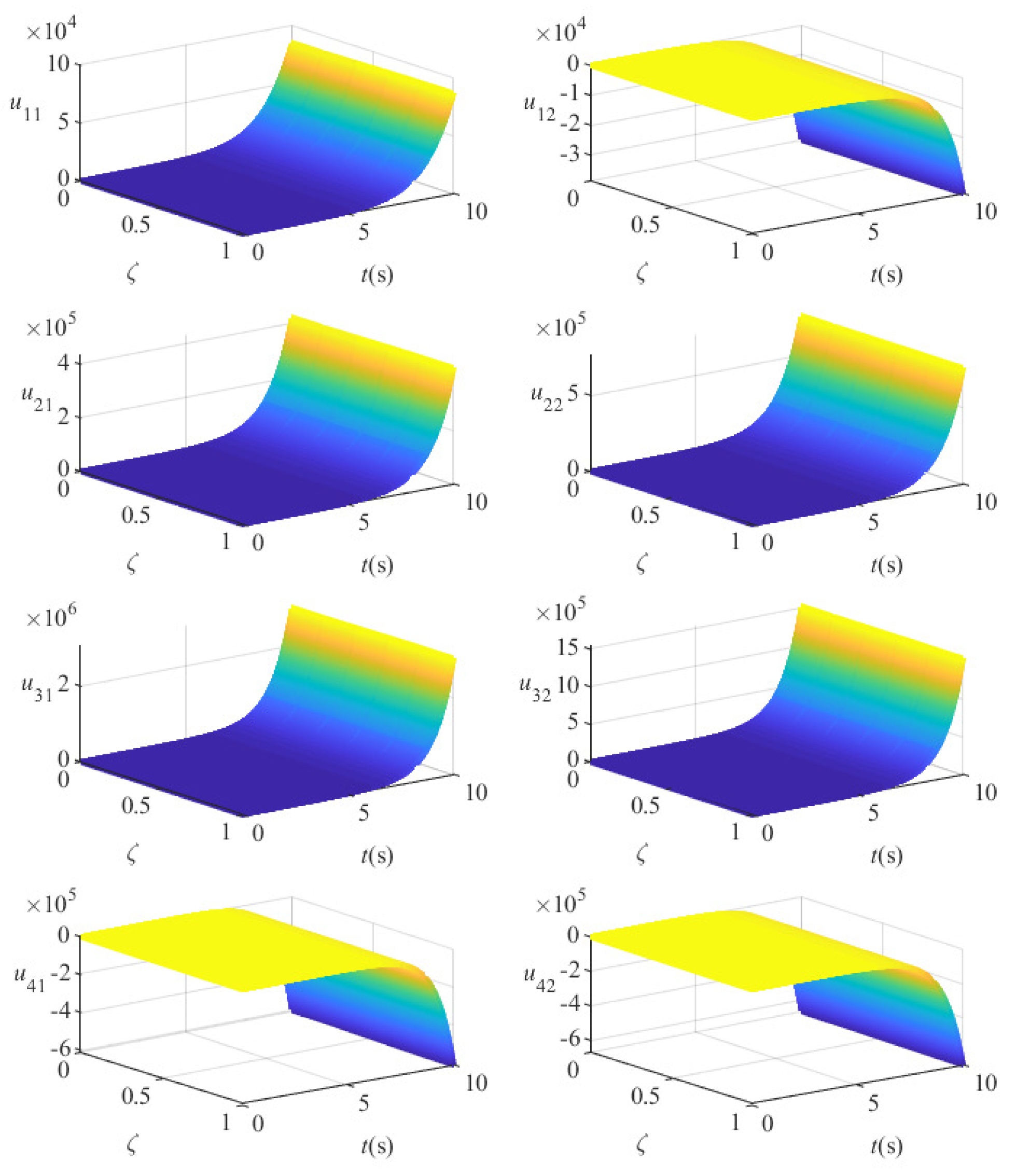
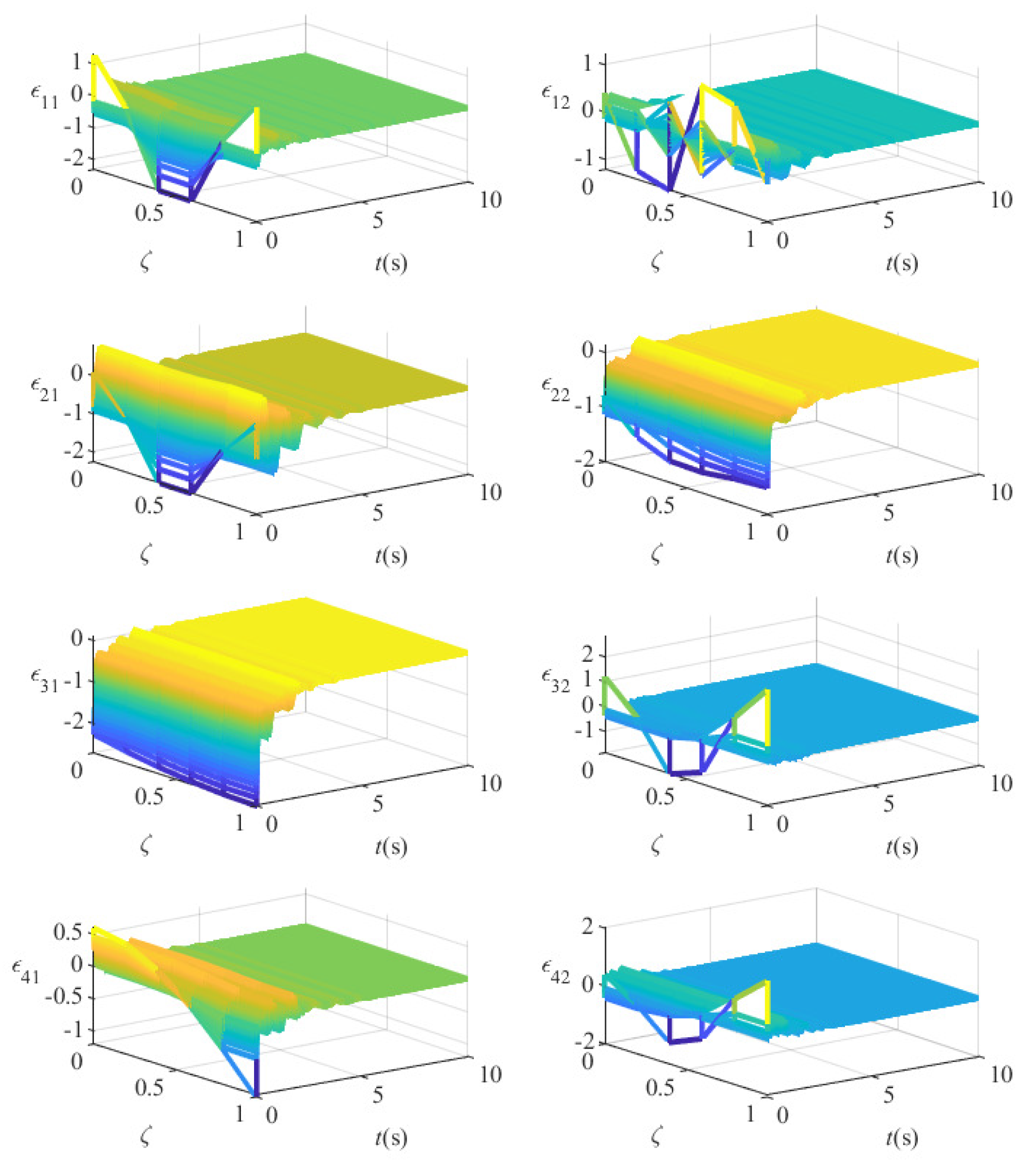
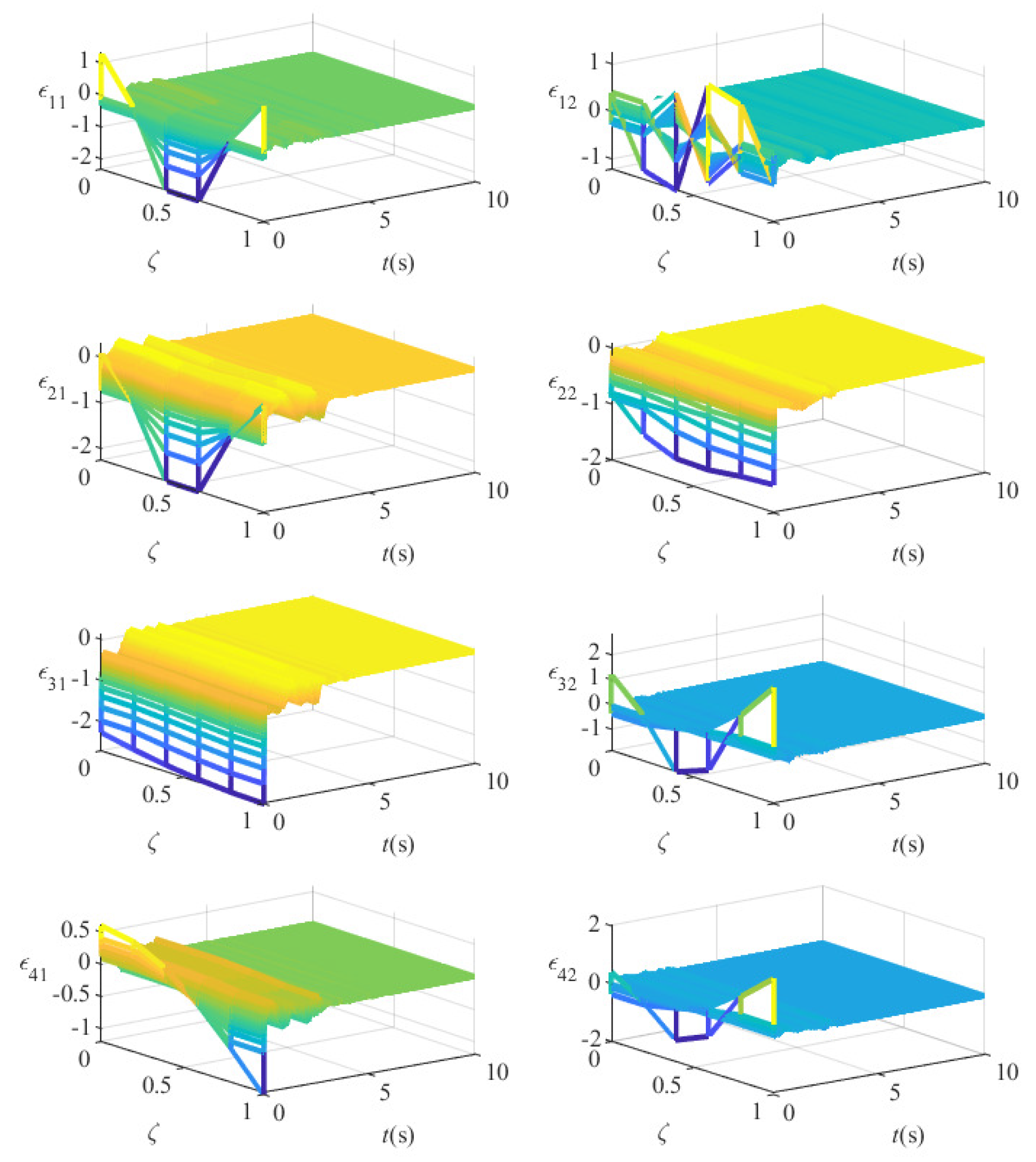
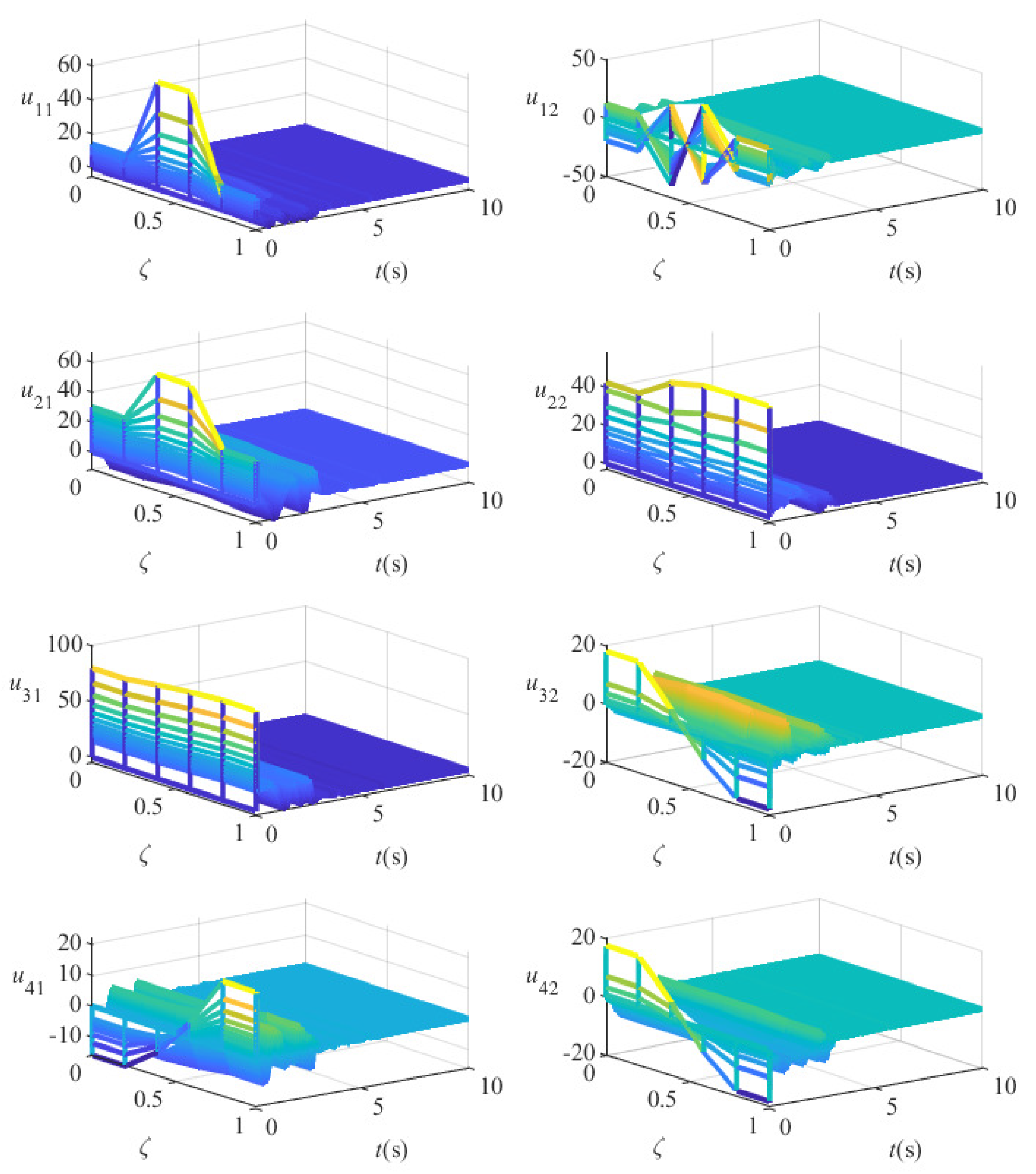
It is shown in Figure 3 that the MTDCSN (1) achieves synchronization with the isolated node (2) under control with the gains (33). The controller is shown in Figure 4.

Example 2.

We consider the MTDCSN (1) with random initial conditions and the same parameters as those in Theorem 1, except:

$$\begin{array}{cc}\hfill & {\tau }_1\left(t\right)=2+sin\left(0.25\pi t\right),{\tau }_2\left(t\right)=1+0.3cos(\pi t+\pi /4),\hfill \\ \hfill & {\tau }_3\left(t\right)=2-exp\left(-t/2\right),{\tau }_4\left(t\right)=2+0.8arctan\left(t\right).\hfill \end{array}$$

(34)

We take $max\{{\tau }_1\left(t\right),{\tau }_2\left(t\right),{\tau }_3\left(t\right),{\tau }_4\left(t\right)\}\le \tau =3$ and $\chi =1$. From (34), it is obvious that ${\mu }_1=0.25\pi$, ${\mu }_2=0.3\pi$, ${\mu }_3=0.5$, ${\mu }_4=0.8$.

From Figure 5, it can be seen that the MTDCSN (1) cannot achieve synchronization without control. According to Theorem 2, solving LMIs (25)–(27) with Matlab, we can obtain: ${\alpha }_1={\alpha }_2={\alpha }_3={\alpha }_4=6.8606$, and

$$\begin{array}{cc}\hfill & R1=\left[\begin{array}{cc}0.9737& -0.0029\\ -0.0029& 0.7897\end{array}\right],R2=\left[\begin{array}{cc}0.9694& -0.0029\\ -0.0029& 0.7887\end{array}\right],\hfill \\ \hfill & R3=\left[\begin{array}{cc}0.9721& -0.0029\\ -0.0029& 0.7893\end{array}\right],R4=\left[\begin{array}{cc}0.9707& -0.0029\\ -0.0029& 0.7890\end{array}\right],\hfill \\ \hfill & S1=\left[\begin{array}{cc}0.9737& -0.0029\\ -0.0029& 0.7897\end{array}\right],S2=\left[\begin{array}{cc}0.9694& -0.0029\\ -0.0029& 0.7887\end{array}\right],\hfill \\ \hfill & S3=\left[\begin{array}{cc}0.9721& -0.0029\\ -0.0029& 0.7893\end{array}\right],S4=\left[\begin{array}{cc}0.9707& -0.0029\\ -0.0029& 0.7890\end{array}\right].\hfill \end{array}$$

(35)

Therefore, the control gains $K_{Pi}$ and $K_{Di}$ are obtained as:

$$\begin{array}{cc}\hfill & K_{P1}=\left[\begin{array}{cc}40.3444& 0.1801\\ 0.1511& 47.6124\end{array}\right],K_{P2}=\left[\begin{array}{cc}40.3914& 0.1813\\ 0.1523& 47.6637\end{array}\right],\hfill \\ \hfill & K_{P3}=\left[\begin{array}{cc}40.3605& 0.1806\\ 0.1516& 47.6307\end{array}\right],K_{P4}=\left[\begin{array}{cc}40.3762& 0.1810\\ 0.1520& 47.6478\end{array}\right],\hfill \\ \hfill & K_{D1}=\left[\begin{array}{cc}1.0000& -0.0002\\ 0.0000& 1.2000\end{array}\right],K_{D2}=\left[\begin{array}{cc}1.0000& -0.0002\\ 0.0000& 1.2000\end{array}\right],\hfill \\ \hfill & K_{D3}=\left[\begin{array}{cc}1.0000& -0.0002\\ 0.0000& 1.2000\end{array}\right],K_{D4}=\left[\begin{array}{cc}1.0000& -0.0002\\ 0.0000& 1.2000\end{array}\right],\hfill \end{array}$$

(36)

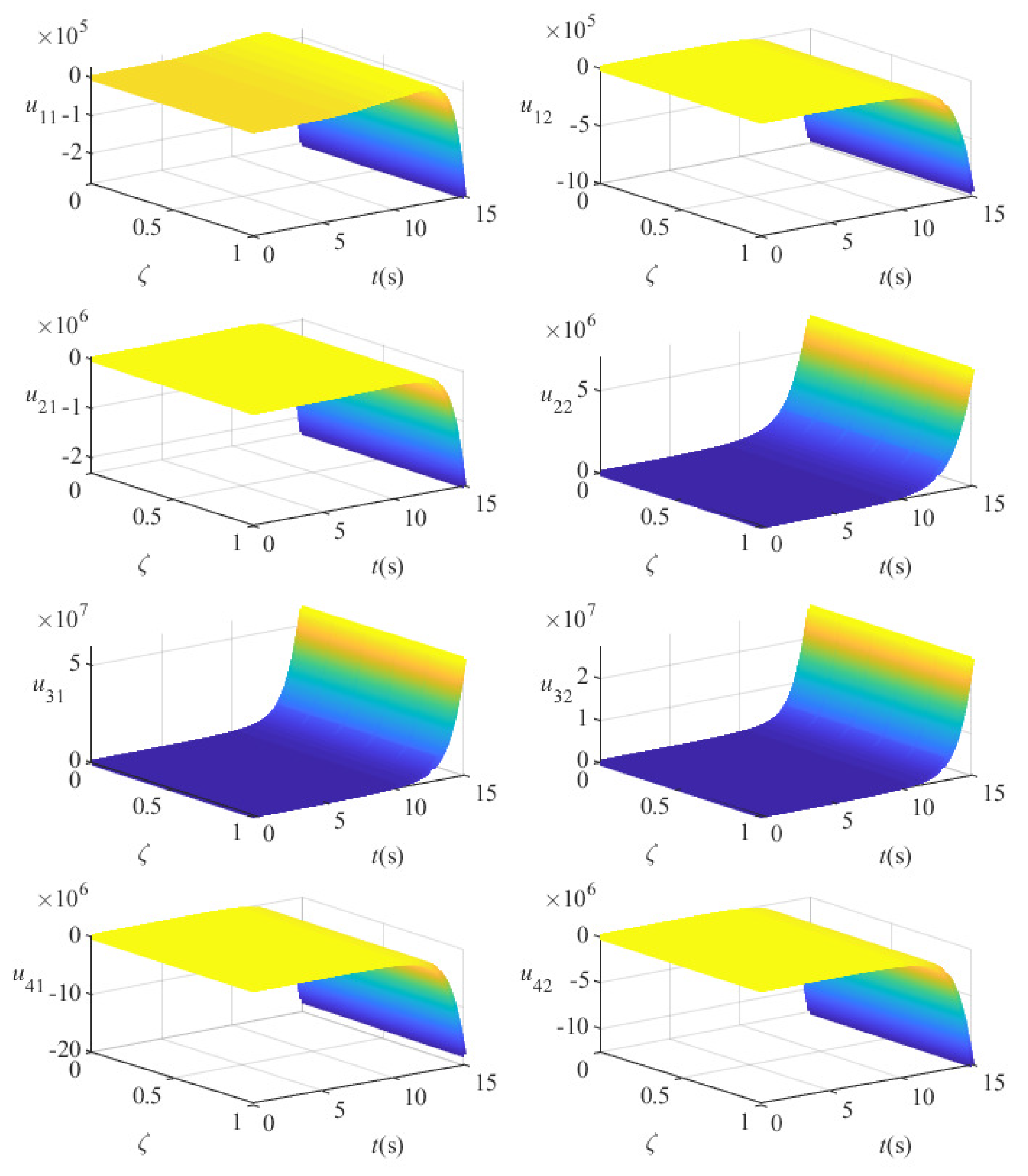
It is shown in Figure 6 that the MTDCSN (1) achieves synchronization with the isolated node (2) under control with the gains (36). The controller is shown in Figure 7.

6. Conclusions

This paper aimed to study the synchronization of a class of nonlinear MTDCSNs. The model was established using coupled semi-linear parabolic PIDEs. P-sD control was employed for the MTDCSN with time-invariant delays and was further used for the MTDCSN with time-varying delays. The synchronization criteria were obtained in terms of LMIs for time-invariant delays and time-varying delays, respectively. An example was used to illustrate the effectiveness of the proposed methods. Compared with other methods, this method not only considers multiple time-invariant and time-varying delays but also deals with PIDE-based complex spatiotemporal networks. In future work, the pinning synchronization of MTDCSNs will be studied.

References

- Hu, C.; He, H.; Jiang, H. Fixed/preassigned-time synchronization of complex networks via improving fixed-time stability. IEEE Trans. Cybern. 2020, 51, 2882–2892. [Google Scholar] [CrossRef]
- Liu, X.; Ho, D.W.; Song, Q.; Xu, W. Finite/fixed-time pinning synchronization of complex networks with stochastic disturbances. IEEE Trans. Cybern. 2018, 49, 2398–2403. [Google Scholar] [CrossRef]
- Gan, L.; Li, S.; Duan, N.; Kong, X. Adaptive output synchronization of general complex dynamical network with time-varying delays. Mathematics 2020, 8, 311. [Google Scholar] [CrossRef] [Green Version]
- Alimi, A.M.; Aouiti, C.; Assali, E.A. Finite-time and fixed-time synchronization of a class of inertial neural networks with multi-proportional delays and its application to secure communication. Neurocomputing 2019, 332, 29–43. [Google Scholar] [CrossRef]
- Shanmugam, L.; Mani, P.; Rajan, R.; Joo, Y.H. Adaptive synchronization of reaction–diffusion neural networks and its application to secure communication. IEEE Trans. Cybern. 2018, 50, 911–922. [Google Scholar] [CrossRef] [PubMed]
- Dong, S.; Zhu, H.; Zhong, S.; Shi, K.; Lu, J. Impulsive-based almost surely synchronization for neural network systems subject to deception attacks. IEEE Trans. Neural Netw. Learn. Syst. 2021. [Google Scholar] [CrossRef] [PubMed]
- Zhang, H.; Li, L.; Li, X. Exponential synchronization of coupled neural networks under stochastic deception attacks. Neural Netw. 2022, 145, 189–198. [Google Scholar] [CrossRef]
- Xing, M.; Lu, J.; Qiu, J.; Shen, H. Synchronization of complex dynamical networks subject to DoS attacks: An improved coding-decoding protocol. IEEE Trans. Cybern. 2021. [Google Scholar] [CrossRef]
- Wen, S.; Zeng, Z.; Huang, T.; Zhang, Y. Exponential adaptive lag synchronization of memristive neural networks via fuzzy method and applications in pseudorandom number generators. IEEE Trans. Fuzzy Syst. 2013, 22, 1704–1713. [Google Scholar] [CrossRef]
- Mani, P.; Rajan, R.; Shanmugam, L.; Joo, Y.H. Adaptive control for fractional order induced chaotic fuzzy cellular neural networks and its application to image encryption. Inf. Sci. 2019, 491, 74–89. [Google Scholar] [CrossRef]
- Feng, Y.; Wang, Y.; Wang, J.W.; Li, H.X. Backstepping-based distributed abnormality localization for linear parabolic distributed parameter systems. Automatica 2022, 135, 109930. [Google Scholar] [CrossRef]
- Wu, H.N.; Zhang, X.M.; Wang, J.W.; Zhu, H.Y. Observer-based output feedback fuzzy control for nonlinear parabolic PDE-ODE coupled systems. Fuzzy Sets Syst. 2021, 402, 105–123. [Google Scholar] [CrossRef]
- Wang, J.W. A unified Lyapunov-based design for a dynamic compensator of linear parabolic MIMO PDEs. Int. J. Control 2021, 94, 1804–1811. [Google Scholar] [CrossRef]
- Kanakov, O.; Osipov, G.; Chan, C.K.; Kurths, J. Cluster synchronization and spatio-temporal dynamics in networks of oscillatory and excitable Luo-Rudy cells. Chaos Interdiscip. J. Nonlinear Sci. 2007, 17, 015111. [Google Scholar] [CrossRef] [PubMed]
- Kakmeni, F.M.; Baptista, M. Synchronization and information transmission in spatio-temporal networks of deformable units. Pramana 2008, 70, 1063–1076. [Google Scholar] [CrossRef] [Green Version]
- Rybalova, E.; Semenova, N.; Strelkova, G.; Anishchenko, V. Transition from complete synchronization to spatio-temporal chaos in coupled chaotic systems with nonhyperbolic and hyperbolic attractors. Eur. Phys. J. Spec. Top. 2017, 226, 1857–1866. [Google Scholar] [CrossRef]
- Yang, C.; Cao, J.; Huang, T.; Zhang, J.; Qiu, J. Guaranteed cost boundary control for cluster synchronization of complex spatio-temporal dynamical networks with community structure. Sci. China Inf. Sci. 2018, 61, 052203. [Google Scholar] [CrossRef] [Green Version]
- Yang, C.; Li, Z.; Chen, X.; Zhang, A.; Qiu, J. Boundary control for exponential synchronization of reaction-diffusion neural networks based on coupled PDE-ODEs. IFAC-PapersOnLine 2020, 53, 3415–3420. [Google Scholar] [CrossRef]
- Tan, X.; Cao, J.; Rutkowski, L. Distributed dynamic self-triggered control for uncertain complex networks with Markov switching topologies and random time-varying delay. IEEE Trans. Netw. Sci. Eng. 2019, 7, 1111–1120. [Google Scholar] [CrossRef]
- Wang, Y.; Tian, Y.; Li, X. Global exponential synchronization of interval neural networks with mixed delays via delayed impulsive control. Neurocomputing 2021, 420, 290–298. [Google Scholar] [CrossRef]
- Yang, S.; Guo, Z.; Wang, J. Global synchronization of multiple recurrent neural networks with time delays via impulsive interactions. IEEE Trans. Neural Netw. Learn. Syst. 2016, 28, 1657–1667. [Google Scholar] [CrossRef] [PubMed]
- Popa, C.A.; Kaslik, E. Finite–time Mittag–Leffler synchronization of neutral–type fractional-order neural networks with leakage delay and time-varying delays. Mathematics 2020, 8, 1146. [Google Scholar] [CrossRef]
- Yao, J.; Wang, H.O.; Guan, Z.H.; Xu, W. Stability and passivity of complex spatio-temporal switching networks with coupling delays. IFAC Proc. 2008, 41, 6638–6641. [Google Scholar] [CrossRef]
- Yao, J.; Wang, H.O.; Guan, Z.H.; Xu, W. Passive stability and synchronization of complex spatio-temporal switching networks with time delays. Automatica 2009, 45, 1721–1728. [Google Scholar] [CrossRef]
- Zhou, D.D.; Guan, Z.H.; Liao, R.Q.; Chi, M.; Xiao, J.W.; Jiang, X.W. Topology identification of a class of complex spatio-temporal networks with time delay. IET Control Theory Appl. 2017, 11, 611–618. [Google Scholar] [CrossRef]
- Zhou, D.D.; Hu, B.; Guan, Z.H.; Liao, R.Q.; Xiao, J.W. Finite-time topology identification of complex spatio-temporal networks with time delay. Nonlinear Dyn. 2018, 91, 785–795. [Google Scholar] [CrossRef]
- Sheng, Y.; Zeng, Z. Impulsive synchronization of stochastic reaction–diffusion neural networks with mixed time delays. Neural Netw. 2018, 103, 83–93. [Google Scholar] [CrossRef]
- Lu, B.; Jiang, H.; Hu, C.; Abdurahman, A. Synchronization of hybrid coupled reaction–diffusion neural networks with time delays via generalized intermittent control with spacial sampled-data. Neural Netw. 2018, 105, 75–87. [Google Scholar] [CrossRef]
- Yang, C.; Huang, T.; Yi, K.; Zhang, A.; Chen, X.; Li, Z.; Qiu, J.; Alsaadi, F.E. Synchronization for nonlinear complex spatio-temporal networks with multiple time-invariant delays and multiple time-varying delays. Neural Process. Lett. 2019, 50, 1051–1064. [Google Scholar] [CrossRef]
- Zhang, R.; Zeng, D.; Park, J.H.; Lam, H.K.; Xie, X. Fuzzy sampled-data control for synchronization of T–S fuzzy reaction–diffusion neural networks with additive time-varying delays. IEEE Trans. Cybern. 2020, 51, 2384–2397. [Google Scholar] [CrossRef]
- Thieme, H.R.; Zhao, X.Q. Asymptotic speeds of spread and traveling waves for integral equations and delayed reaction–diffusion models. J. Differ. Equ. 2003, 195, 430–470. [Google Scholar] [CrossRef] [Green Version]
- Yang, X.; Yu, J.; Xu, M.; Fan, W. Convertible bond pricing with partial integro-differential equation model. Math. Comput. Simul. 2018, 152, 35–50. [Google Scholar] [CrossRef]
- Volpert, V.; Petrovskii, S. Reaction–diffusion waves in biology. Phys. Life Rev. 2009, 6, 267–310. [Google Scholar] [CrossRef] [PubMed]
- Halatek, J.; Frey, E. Rethinking pattern formation in reaction–diffusion systems. Nat. Phys. 2018, 14, 507–514. [Google Scholar] [CrossRef]
- Ebenbeck, M.; Knopf, P. Optimal control theory and advanced optimality conditions for a diffuse interface model of tumor growth. ESAIM Control Optim. Calc. Var. 2020, 26, 71. [Google Scholar] [CrossRef]
- Deutscher, J.; Kerschbaum, S. Backstepping control of coupled linear parabolic PIDEs with spatially varying coefficients. IEEE Trans. Autom. Control 2018, 63, 4218–4233. [Google Scholar] [CrossRef] [Green Version]
- Deutscher, J.; Kerschbaum, S. Robust output regulation by state feedback control for coupled linear parabolic PIDEs. IEEE Trans. Autom. Control 2019, 65, 2207–2214. [Google Scholar] [CrossRef]
- Liu, W.W.; Wang, J.M.; Guo, W. A backstepping approach to adaptive error feedback regulator design for one-dimensional linear parabolic PIDEs. J. Math. Anal. Appl. 2021, 503, 125310. [Google Scholar] [CrossRef]
- Seuret, A.; Gouaisbaut, F. Jensen’s and Wirtinger’s inequalities for time-delay systems. IFAC Proc. 2013, 45, 343–348. [Google Scholar] [CrossRef] [Green Version]
- Yang, C.; Zhang, A.; Zhang, X.; Liu, Z.; Pang, G.; Qiu, J.; Wen, Y.; Shanshui, S.; Cao, J. SPID control for synchronization of complex PIDE networks with time delays. In Proceedings of the IECON 2017-43rd Annual Conference of the IEEE Industrial Electronics Society, Beijing, China, 29 October–1 November 2017; pp. 5997–6001. [Google Scholar]
Figure 1.
The structure of the P-sD controller (3).
Figure 2.
of the multiple time-delayed complex spatiotemporal network (MTDCSN) without control in Example 1.
Figure 3.
of the MTDCSN with control in Example 1.
Figure 4.
The controller in Example 1.
Figure 5.
of the MTDCSN without control in Example 2.
Figure 6.
of the MTDCSN with control in Example 2.
Figure 7.
The controller in Example 2.
Publisher’s Note: MDPI stays neutral with regard to jurisdictional claims in published maps and institutional affiliations. |
© 2022 by the authors. Licensee MDPI, Basel, Switzerland. This article is an open access article distributed under the terms and conditions of the Creative Commons Attribution (CC BY) license (https://creativecommons.org/licenses/by/4.0/).
Share and Cite
MDPI and ACS Style
Dai, J.; Yang, C. Synchronization of Nonlinear Complex Spatiotemporal Networks Based on PIDEs with Multiple Time Delays: A P-sD Method. Mathematics 2022, 10, 509. https://0-doi-org.brum.beds.ac.uk/10.3390/math10030509
AMA Style
Dai J, Yang C. Synchronization of Nonlinear Complex Spatiotemporal Networks Based on PIDEs with Multiple Time Delays: A P-sD Method. Mathematics. 2022; 10(3):509. https://0-doi-org.brum.beds.ac.uk/10.3390/math10030509
Chicago/Turabian StyleDai, Jiashu, and Chengdong Yang. 2022. "Synchronization of Nonlinear Complex Spatiotemporal Networks Based on PIDEs with Multiple Time Delays: A P-sD Method" Mathematics 10, no. 3: 509. https://0-doi-org.brum.beds.ac.uk/10.3390/math10030509
Note that from the first issue of 2016, this journal uses article numbers instead of page numbers. See further details here.