Identification of Homogeneous Groups of Actors in a Local AHP-Multiactor Context with a High Number of Decision-Makers: A Bayesian Stochastic Search

Abstract

The identification of homogeneous groups of actors in a local AHP-multiactor context based on their preferences is an open problem, particularly when the number of decision-makers is high. To solve this problem in the case of using stochastic AHP, this paper proposes a new Bayesian stochastic search methodology for large-scale problems (number of decision-makers greater than 20). The new methodology, based on Bayesian tools for model comparison and selection, takes advantage of the individual preference structures distributions obtained from stochastic AHP to allow the identification of homogeneous groups of actors with a maximum common incompatibility threshold. The methodology offers a heuristic approach with several near-optimal partitions, calculated by the Occam’s window, that capture the uncertainty that is inherent when considering intangible aspects (AHP). This uncertainty is also reflected in the graphs that show the similarities of the decision-maker’s opinions and that can be used to achieve representative collective positions by constructing agreement paths in negotiation processes. If a small number of actors is considered, the proposed algorithm (AHP Bayesian clustering) significantly reduces the computational time of group identification with respect to an exhaustive search method. The methodology is illustrated by a real case of citizen participation based on e-Cognocracy.

1. Introduction

The incorporation into formal models of the rational associated with the traditional scientific method and the emotional associated with the human factor is one of the most outstanding challenges faced by decision sciences in the Knowledge Society (KS). The resolution of complex problems posed in this context (KS) requires the development of new analytical and computing tools that make it possible to take advantage of the talent, experience, and collaborative nature of the human being together with the potential of information and communication technology (ICT).

The Analytic Hierarchy Process (AHP) [1] is one of the most extended multicriteria decision-making techniques that best respond to these challenges; its suitability to work with intangible aspects and with multiple actors are two of its most appreciated characteristics. AHP integrates the subjective, intangible, and emotional through the judgements elicited when evaluating the pairwise comparison matrices (PCMs) contemplated in the problem. Escobar et al. [2] consider three scenarios when dealing with multiactor decisions: Group Decision Making (GDM) [3]; Negotiated Decision Making (NDM) [4] and Systemic Decision Making (SDM) [5].

Assuming a local (single criterion) AHP-multiactor decision making context, we will go on to analyse a classical and still unresolved problem: the compatibility between the individuals and the collective positions or preferences when the number of actors is medium or high.

In a previous work [3], we established the stochastic AHP framework, based on Bayesian analysis, used for solving this problem for a reduced number of actors (fewer than 12). We also proposed an exhaustive search algorithm for the identification of groups of actors that present homogeneous and differentiated behaviours, and a semi-automatic procedure for the aggregation of the priorities of the nearby groups to reach collective positions with the greatest possible consensus.

In a local AHP decision making context, the consideration of a stochastic approach for the identification of homogeneous groups of actors in terms of their priorities is justified by the need to incorporate into the formal models the actors’ uncertainty that is inherent when working with intangible aspects; one of the highlighted characteristics of AHP. In this context, to deal with this uncertainty and with that derived from the acceptable inconsistency allowed for the decision-makers, it is more appropriate to consider stochastic than deterministic approaches.

For a number of decision-makers greater than 20, that is to say, for a large-scale number of actors [6], the complexity of the problem (hard NP) does not allow resorting us to resort to exhaustive search algorithms in the determination of homogenous groups and, therefore, this is an open problem.

To deal with these large-scale situations, we propose the use of stochastic search procedures, based on Bayesian tools for model comparison and selection, that take advantage of the individual preference structures distributions obtained from stochastic AHP to allow the identification of homogeneous groups of actors with a maximum common incompatibility threshold. This kind of Bayesian tools has been shown to be very effective in variables selection problems given that they tend to select parsimonious models with good fitness to data (see, for instance, [7,8,9,10,11] and the recent review of [12]).

The new methodology, named in what follows as AHP Bayesian clustering (AHP-BYC), is inspired by the main ideas of [9] and applies them to identify the best partitions of the set of decision-maker. It uses alpha and gamma distributions (preference structures associated to decision-makers) to carry out a more efficient pseudo-random exploration of the partitions space. The approach employs the factor Bayes [13] as model (partition) comparison tool and calculates the Occam’s window [7] to select partitions that describe, in a parsimonious way, the different opinions of the actors involved in the problem. The search procedure uses a random combination of cluster divisive and agglomerative steps to explore the partitions space. Some of these steps are specific to the AHP context and allow the computational time to be improved. In addition, a visual procedure based on the use of graphs is introduced to analyze the preference structures of the selected partition and the similarities of the decision-maker’s opinions. Both, preference structures and opinions, have been obtained from the different partitions included in the Occam’s window. In this way, the graphs reflect the uncertainty associated with the partition selection process. The AHP-BYC methodology is illustrated by a practical example.

This work contributes to literature on the identification of homogeneous groups in decision making problems using AHP in two ways: (a) It proposes a stochastic search algorithm (AHP-BYC) that combines classical hierarchical steps with a probabilistic evaluation of the quality of the explored partitions, and provides a more efficient and rigorous classification procedure; (b) It also presents a visual representation, based on graphs that analyse the similarity of the decision-makers’ opinions, which makes it easier to find lines of negotiation among the decision-makers in order to achieve representative agreements.

The paper is structured as follows: Section 2 contains a brief review of the literature; Section 3 sets up the problem and describes the algorithm used to solve it; Section 4 applies the methodology to a case study; and Section 5 concludes by highlighting the most relevant aspects of the work and possible extensions.

2. Background

2.1. The Analytic Hierarchy Process

AHP [1] is a mathematical theory of domination that allows the resolution of complex problems involving multiple scenarios, actors, and criteria, incorporating in the model the subjective aspects associated with the human factor together with the objective aspects inherent to the traditional scientific method. For this purpose, by means of a hierarchical modelling of the problem, the use of pairwise comparisons for the incorporation of the intangible or emotional aspects, and a prioritisation process, the total priorities of the alternatives measured on a ratio scale are derived. These priorities reflect on an abstract scale the relative importance of the alternatives according to the relevant attributes of the problem; their values allow the alternatives to be ordered and the best one to be selected.

The AHP methodology consists of three stages: (i) Modelling: construction of a hierarchical model that collects the relevant aspects of the problem (goal, criteria, sub-criteria for different levels, attributes, and alternatives) at the different levels; (ii) Valuation: incorporation of the preferences of the actors by eliciting, using the Saaty’s fundamental scale, the judgments of the PCMs for each node of the hierarchy; (iii) Prioritization and Synthesis: calculation of the local priorities, using a prioritization procedure, and the global priorities, by means of the hierarchical composition principle, for each of the elements (nodes) of the hierarchy, and the total priorities of the considered alternatives following an aggregation synthesis.

One of the most outstanding features of AHP is that it allows us to evaluate the inconsistency of the decision-maker when eliciting the judgments in the PCM built in each node of the hierarchy. As Saaty suggests, it is not necessary for these judgments to be perfectly consistent or cardinally transitive. A PCM R_(nxn) = (r_ij) is consistent [1] if it verifies the cardinal transitivity of the judgments, that is, r_ij r_jk = r_ik ∀ i, j, k = 1, …, n. Otherwise, the matrix is said to be inconsistent. The two most used indicators for measuring the level of inconsistency are the Saaty Consistency Ratio (CR) [1] and the Geometric Consistency Index (GCI) [14,15]. The values of CR < 5% for n = 3; CR < 8% for n = 4, and CR < 10% for n > 4 are considered as acceptable levels of inconsistency. The associated thresholds for GCI are [15]: GCI < 0.31 for n = 3, GCI < 0.35 for n = 4, and GCI < 0.37 for n > 4.

2.2. Multi-Actor Decision Making

In multi-actor decision making, three main approaches are distinguished [5]: (i) Group Decision Making (GDM); (ii) Negotiated Decision Making (NDM) and (iii) Systemic Decision Making (SDM).

In Group Decision Making (GDM), actors work as a single entity, proposing a position agreed upon by all when determining collective priorities [2]. In Negotiated Decision Making (NDM), actors work individually, seeking areas of agreement among themselves [4,16] as a starting point for the negotiation process. Finally, in Systemic Decision Making (SDM), the actors pose a joint position incorporating in a holistic view the actors’ individual preferences on a fixed set of alternatives. This approach integrates all the preferences, even if they are encapsulated in different individual theoretical models or approaches; the only requirement is that they must be expressed as some kind of probability distribution [5].

The procedures used to calculate collective priorities can be grouped as: (i) construction of a collective consensus matrix that can be automatic, semiautomatic or personal; the Aggregations of Individual Judgments (AIJ) and the consensus matrices based on consistency (CCM, PCCM…) are some of the most extended methods; (ii) Aggregation of Individual Priorities (AIP); (iii) Aggregation of Individual Preference Structures (AIPS) and (iv) methods based on stochastic models; the Bayesian Prioritization Procedure (BPP) is one of the best known.

The first group of procedures constructs a consensus matrix, combining in each of its cell expressions based on the individual judgments of that position. The AIJ method [1] assigns the geometric mean of the judgments to each cell, while the CCM [17] assigns the common consistency stability interval and the PCCM [18] latter interval but improved.

Both AIP [19,20] and AIPS [2] work directly with individual priorities; in the first case (AIP) in a deterministic context and in the second (AIPS) in a stochastic context. Finally, the Bayesian Prioritization Procedure (BPP) is also framed in a stochastic context and is based on the use of Bayesian hierarchical models that describe the relationships between the priorities of the group and the judgments issued by its members. The estimation of the group’s priorities is carried out by applying Bayes’ Theorem which incorporates into the estimation process the uncertainty associated with the inconsistency existing in the process of issuing paired comparisons [4,16].

All these procedures assume that the preferences of the decision-makers in the group are homogeneous in the sense that the compatibility between each decision-maker’s preferences and the collective preferences are acceptable [21]. This fact may be clearly unrealistic, especially when the number of actors is large. In this case, it is quite possible that there are different groups of decision-makers with diverse opinions. The identification of these groups as well as the estimation of their priorities becomes a relevant problem that we will address in this work.

Some papers in relevant literature combine the use of cluster and AHP techniques to determine the number of groups in a data set, but they are not fully adapted to our stochastic context. Therefore, [22] uses AHP to select information criteria that determine the optimal number of groups in a large data set. They also use cluster techniques within AHP [23] but, in this case, to reduce an excessively high number of alternatives. Other proposals closer to our problem are [24,25], but both are carried out within a deterministic context, so they are not directly comparable with our proposal.

Unlike these papers, our algorithm is based on a new stochastic search procedure that combines randomly classical divisive and agglomerative steps with a Bayesian probabilistic evaluation of the quality of the explored partitions. The AHP-BYC methodology provides a more efficient and rigorous classification procedure. Some of the previous steps are specific to the stochastic AHP context and make the algorithm very efficient with significantly lower computational times.

3. Methodology

This section shows the methodology used to carry out the identification of homogeneous preference groups in a local AHP-multiactor context (one criterion) with a high number of decision-makers, as well as to estimate the preferences of these groups and to analyse their homogeneity. To do this, a hierarchical Bayesian statistical approach is adopted, based on the use of log-linear models like those used in references [3,16]. These models describe the process of eliciting judgments by the decision-makers of a group. Applying Bayes’ Theorem, for each group, both the posterior distribution of its priorities and its degree of compatibility are calculated. Finally, Bayesian model selection and comparison techniques are applied to determine the best partitions into groups of the set of decision-makers. For this purpose, we describe a new stochastic search algorithm.

3.1. Problem Formulation

First, the log-linear model that is used to determine the priorities of the groups of decision-makers is explained. In what follows [3], N (µ, σ) denotes the univariate normal distribution of mean µ and standard deviation σ; N_p (µ, ∑) denotes the p-variant normal distribution of mean vector µ and the matrix of variances and covariances ∑; T_p (µ, ∑, υ) denotes the p-variant Student t distribution with mean vector µ, scale matrix ∑ and degrees of freedom υ; Gam(p, a) denotes the gamma distribution with shape parameter p and scale parameter 1/a; ${\chi }_{\nu }^2$ denotes the chi-squared distribution with υ degrees of freedom; I_A denotes the indicator function of set A; ∝ indicates proportional to; and [Y|X] denotes the density function of the conditional distribution of Y given X.

Let D = $\left\{{\mathrm{D}}^{[1]},\dots ,{\mathrm{D}}^{[\mathrm{K}]}\right\}$ be the set of decision-makers, A = $\left\{{\mathrm{A}}_1,\dots ,{\mathrm{A}}_{\mathrm{n}}\right\}$ be the set of n alternatives and R^(k) = $\left({\mathrm{r}}_{\mathrm{i}\mathrm{j}}^{(\mathrm{k})}\right)$; k = 1, …, K be the nxn pairwise comparison matrices (PCMs) elicited by each decision-maker. Let ℘(D) the set of partitions of D.

Without loss of generality, we assume that the PCMs are complete; meaning that all paired comparisons have been made. If some of the (i,j) comparisons are missing, the proposed methodology could be analogously adapted, as shown in reference [16].

Let $𝒢$ = $\left\{{\mathbf{G}}_1,\dots ,{\mathbf{G}}_{\mathrm{m}}\right\}$ be a partition of D, with G_g = $\left\{{\mathrm{D}}_{}^{\left[{\mathrm{i}}_{\mathrm{g},\mathrm{1}}\right]},\dots ,{\mathrm{D}}_{}^{\left[{\mathrm{i}}_{\mathrm{g},{\mathrm{n}}_{\mathrm{g}}}\right]}\right\}$ ⊆ D; n_g the size of group G_g for g = 1,…, m, G_g ∩ G_g′ = ∅ if g ≠ g′, ${\displaystyle \underset{\mathrm{g}=1}{\overset{\mathrm{m}}{\cup }}{\mathbf{G}}_{\mathrm{g}}}$ = D; [i_g,j] the j-th (j = 1, …,n_g) decision-maker of group G_g.

In order to avoid identifiability problems, we assume that 1 ≤ ${\mathrm{i}}_{\mathrm{g},1}$ < … < ${\mathrm{i}}_{\mathrm{g},{\mathrm{n}}_{\mathrm{g}}}$ ≤ K and that i_g,1 < i_g′,1 if g < g′.

To obtain the group’s priorities from a Bayesian perspective, a multiplicative model M($𝒢$) with log-normal errors is used [3,16]. The model M($𝒢$) assumes that the decision-makers who belong to a group G_g of the partition $𝒢$ have homogeneous preferences regarding the priorities of the alternatives of A so that:

$${\mathrm{y}}_{\mathrm{i}\mathrm{j}}^{(\mathrm{k})}={\mathsf{\mu }}_{\mathrm{i}}^{(\mathrm{g}(\mathrm{k}))}-{\mathsf{\mu }}_{\mathrm{j}}^{(\mathrm{g}(\mathrm{k}))}+{\mathsf{\epsilon }}_{\mathrm{i}\mathrm{j}}^{(\mathrm{k})};\mathrm{k}=1,\dots ,\mathrm{K};1\le \mathrm{i}<\mathrm{j}\le \mathrm{n};$$

(1)

with ${\mathrm{y}}_{\mathrm{i}\mathrm{j}}^{(\mathrm{k})}=\log \left({\mathrm{r}}_{\mathrm{i}\mathrm{j}}^{(\mathrm{k})}\right)$, where:

(a)

D^[k] ∈ G_g(k) with g(k) ∈ {1, …, m} being the index of the group of $𝒢$ which contains D^[k]

(b)

${\mathsf{\mu }}_{\mathrm{i}}^{\left(\mathrm{g}(\mathrm{k})\right)}=\log \left({\mathrm{v}}_{\mathrm{i}}^{\left(\mathrm{g}(\mathrm{k})\right)}\right)$; i = 1, …, n being ${\mathrm{v}}_{\mathrm{i}}^{\left(\mathrm{g}(\mathrm{k})\right)}$ the priority (without normalising) given to the alternative A_i by the members of the group G_g(k)

(c)

${\mathrm{v}}_{\mathrm{n}}^{\left(\mathrm{g}(\mathrm{k})\right)}=1$ (that is to say, ${\mathsf{\mu }}_{\mathrm{n}}^{\left(\mathrm{g}(\mathrm{k})\right)}=0$) to avoid identifiability problems

(d)

${\mathsf{\epsilon }}_{\mathrm{i}\mathrm{j}}^{(\mathrm{k})}~\mathrm{N}\left(0,{\mathsf{\sigma }}^{(\mathrm{g}(\mathrm{k}))}\right)$; k = 1, …, K; 1 ≤ i < j ≤ n independent.

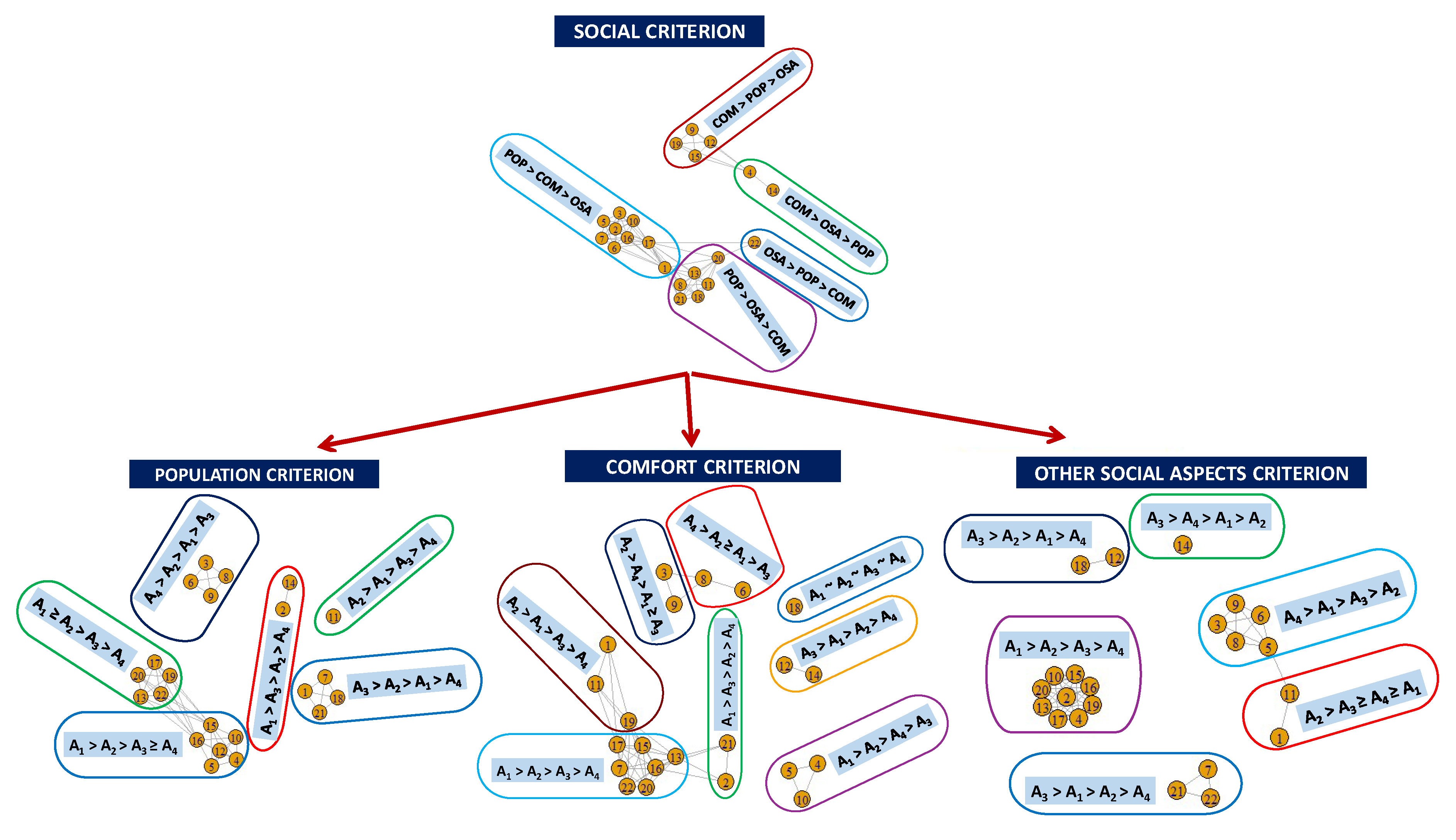
3.2. Analysis of the Priorities and the Homogeneity of the Groups of $𝒢$

The normalised priorities of the group G_g (g = 1,…, m) will be given by the vector:

$${\mathbf{w}}^{\left(\mathrm{g}\right)}={\left({\mathrm{w}}_{\mathrm{i}}^{\left(\mathrm{g}\right)};\mathrm{i}=1,\dots ,\mathrm{n}\right)}^{\prime } \mathrm{where} {\mathrm{w}}_{\mathrm{i}}^{\left(\mathrm{g}\right)}=\frac{{\mathrm{v}}_{\mathrm{i}}^{\left(\mathrm{g}\right)}}{{\displaystyle \sum _{\mathrm{i}=1}^{\mathrm{n}}{\mathrm{v}}_{\mathrm{i}}^{\left(\mathrm{g}\right)}}}; \mathrm{i}=1, \dots , \mathrm{n}.$$

In addition, the level of the compatibility of the groups of $𝒢$ will be measured by the error standard deviation {σ^(g); g = 1, …, m} which quantifies the level of compatibility of each decision-maker with the priorities vector w^(g) of his/her group. The estimation of (w(g), σ^(g)) is carried out using a Bayesian approach which let us obtain exact inferences about them. To do this, we use the standard conjugate normal-gamma prior distributions given by:

$${\mathsf{\mu }}^{\left(\mathrm{g}\right)}={\left({\mathsf{\mu }}_1^{\left(\mathrm{g}\right)},\dots ,{\mathsf{\mu }}_{\mathrm{n}-1}^{\left(\mathrm{g}\right)}\right)}^{\prime }|{\mathsf{\tau }}^{(\mathrm{g})}~{\mathrm{N}}_{\mathrm{n}-1}\left(0,\frac{1}{{\mathrm{c}}_0{\mathsf{\tau }}^{(\mathrm{g})}}{I}_{\mathrm{n}-1}\right) \mathrm{with} {\mathrm{c}}_0>0$$

(2)

$${\mathsf{\tau }}^{(\mathrm{g})}=\frac{1}{{\mathsf{\sigma }}^{\left(\mathrm{g}\right)2}} ~ \mathrm{Gam}\left(\frac{{\mathrm{n}}_0}{2},\frac{{\mathrm{n}}_0{\mathrm{s}}_0^2}{2}\right)$$

(3)

The constants ${\mathrm{c}}_0$, ${\mathrm{n}}_0$, and ${\mathrm{s}}_0^2$ determine the degree of strength of the prior distribution. In the illustrative example we have taken [3] ${\mathrm{c}}_0$ = 0.1 so that the influence of the prior distribution of µ^(G) is not significant. The hyper-parameters ${\mathrm{n}}_0$ and ${\mathrm{s}}_0^2$ are determined from the maximum levels of incompatibility ${\mathsf{\sigma }}_{\max }^2$ allowed for each decision-maker so that:

$$\mathrm{P}\left[0\le {\mathsf{\sigma }}^{\left(\mathrm{g}\right)2}\le {\mathsf{\sigma }}_{\max }^2\right]=1-\mathsf{\alpha }$$

being, 1 − α (0 < α < 1) the level of credibility that we want to achieve. The value of ${\mathsf{\sigma }}_{\max }^2$ has been set using the thresholds of the geometric consistency index (GCI) proposed by [15]. In our illustrative example, and given that n = 4, we take ${\mathsf{\sigma }}_{\max }^2$ = 0.35 and α = 0.05, which resulted in ${\mathrm{n}}_0$ = 0.1 and ${\mathrm{s}}_0^2$ = 0.0014.

3.2.1. Posterior Distribution

Using Bayes’ theorem, and taking into account (1)–(3), the posterior distribution of (µ^(g),τ^(g)) is given by:

$$\begin{array}{c}{\mathsf{\mu }}^{(\mathrm{g})}| \{\mathbf{y}\left(\mathrm{k}\right); \mathrm{k}\in \{1, \dots , \mathrm{K}\}: \mathrm{g}\left(\mathrm{k}\right)=\mathrm{g}\} ~\\ {\mathrm{T}}_{\mathrm{n}-1}\left({\mathbf{m}}^{\left(\mathrm{g}\right)},{\mathrm{s}}^{\left(\mathrm{g}\right)2}{\left({\mathrm{n}}_{\mathrm{g}}\left(\mathbf{X}{}^{\prime }\mathbf{X}\right)+{\mathrm{c}}_0{\mathrm{I}}_{\mathrm{n}-1}\right)}^{-1},{\mathrm{n}}_0+\mathrm{J}{\mathrm{n}}_{\mathrm{g}}\right)\end{array}$$

(4)

$${\mathsf{\tau }}^{(\mathrm{g})}|\{{\mathbf{y}}^{\left(\mathrm{k}\right)}; \mathrm{k}\in \{1, \dots , \mathrm{K}\}: \mathrm{g}\left(\mathrm{k}\right)=\mathrm{g}\} ~ \mathrm{Gam}\left(\frac{{\mathrm{n}}_0+\mathrm{J}{\mathrm{n}}_{\mathrm{g}}}{2},\left(\frac{{\mathrm{n}}_0+\mathrm{J}{\mathrm{n}}_{\mathrm{g}}}{2}\right){\mathrm{s}}^{\left(\mathrm{g}\right)2}\right)$$

(5)

for g = 1, …,m where y^(k) = ${\left({\mathrm{y}}_{\mathrm{i}\mathrm{j}}^{(\mathrm{k})};1\le \mathrm{i}<\mathrm{j}\le \mathrm{n}\right)}^{\prime }$ for k = 1, …, K and X = (x_ij) (J × (n − 1)) with J = $\frac{\mathrm{n}(\mathrm{n}-1)}{2}$ is the regression matrix of model (1) so that:

-

x_ij = 1 if the i-th judgement is y_jk with k ≠ j;

-

x_ij = −1 if the i-th judgement is y_kj with k ≠ j;

-

x_ij = 0 in any other case.

$$\begin{gathered} {\mathbf{m}}^{(\mathrm{g})}={\left({\mathrm{n}}_{\mathrm{g}}\left(\mathbf{X}{}^{\prime }\mathbf{X}\right)+{\mathrm{c}}_0{\mathrm{I}}_{\mathrm{n}-1}\right)}^{-1}\left(\mathbf{X}{}^{\prime }\left({\displaystyle \sum _{\mathrm{k}:\mathrm{g}(\mathrm{k})=\mathrm{g}}^{}{\mathbf{y}}^{(\mathrm{k})}}\right)\right) \\ {\mathrm{s}}^{(\mathrm{g})2}=\frac{{\mathrm{n}}_0{\mathrm{s}}_0^2+{\displaystyle \sum _{\mathrm{k}:\mathrm{g}\left(\mathrm{k}\right)=\mathrm{g}}{\mathbf{y}}^{(\mathrm{k}){}^{\prime }}{\mathbf{y}}^{(\mathrm{k})}}-{\mathbf{m}}^{\left(\mathrm{g}\right){}^{\prime }}\left({\mathrm{n}}_{\mathrm{g}}\left(\mathbf{X}{}^{\prime }\mathbf{X}\right)+{\mathrm{c}}_0{\mathrm{I}}_{\mathrm{n}-1}\right){\mathbf{m}}^{\left(\mathrm{g}\right)}}{{\mathrm{n}}_0+\mathrm{J}{\mathrm{n}}_{\mathrm{g}}} \end{gathered}$$

The proof of these results can be seen in reference [3]. From the posterior distributions (4) and (5), point and credibility interval estimations of ${\mathsf{\mu }}^{(\mathrm{g})}$ and σ^(g) using the posterior median and the corresponding posterior quantiles can be obtained. In addition, and using Monte Carlo, for each group {G_g; g = 1, …, m} the posterior distribution of their priorities vectors {w^(g); g = 1, …, m} could be calculated (see reference [3] for details).

Furthermore, information about the most preferred alternative (P.α problem) of each group G_g could also be calculated using the alpha distributions ${\mathbf{P}}_{\mathsf{\alpha }}^{{\mathbf{G}}_{\mathrm{g}}}=\left({\mathrm{P}}_{\mathsf{\alpha },1}^{{\mathbf{G}}_{\mathrm{g}}},\dots ,{\mathrm{P}}_{\mathsf{\alpha },\mathrm{n}}^{{\mathbf{G}}_{\mathrm{g}}}\right)$ with:

$${\mathrm{P}}_{\mathsf{\alpha },\mathrm{i}}^{\mathbf{G}}=\mathrm{P}\left[{\mathrm{w}}_{\mathrm{i}}^{(\mathrm{G})}={\max }_{1\le \mathrm{j}\le \mathrm{n}}{\mathrm{w}}_{\mathrm{j}}^{(\mathrm{G})}|\left\{{\mathbf{y}}^{(\mathrm{k})};\mathrm{k}=1,\dots ,\mathrm{K}\right\}\right]; \mathrm{i}=1, \dots , n$$

(6)

and about the most preferred ranking of alternatives (P.γ problem) using the gamma distributions ${\mathbf{P}}_{\mathsf{\gamma }}^{{\mathbf{G}}_{\mathrm{g}}}=\left({\mathrm{P}}_{\mathsf{\gamma },1}^{{\mathbf{G}}_{\mathrm{g}}},\dots ,{\mathrm{P}}_{\mathsf{\gamma },\mathrm{n}!}^{{\mathbf{G}}_{\mathrm{g}}}\right)$ with

$${\mathrm{P}}_{\mathsf{\gamma },{\mathsf{\gamma }}_{\mathrm{h}}}^{\mathbf{G}}=\mathrm{P}\left[{\mathrm{w}}_{{\mathsf{\gamma }}_{\mathrm{h},1}}^{(\mathrm{G})}\le \dots \le {\mathrm{w}}_{{\mathsf{\gamma }}_{\mathrm{h},\mathrm{n}}}^{(\mathrm{G})}|\left\{{\mathbf{y}}^{(\mathrm{k})};\mathrm{k}=1,\dots ,\mathrm{K}\right\}\right]; \mathrm{h}=1, \dots , n!$$

(7)

where γ_h = (γ_h,1, …, γ_h,n) is the h-th permutation of the elements of A sorted according to the lexicographical order (see references [3,16] for more details).

3.2.2. Analysis of the Representativeness of a Partition $𝒢$

The evaluation of the representativeness of a partition $𝒢$ = $\left\{{\mathbf{G}}_1,\dots ,{\mathbf{G}}_{\mathrm{m}}\right\}$ is carried out using the prior marginal density [Y| $𝒢$] where Y = {y^(k); k ∈ {1, …, K}}. This density evaluates the goodness of fit of the model (1)–(3) with respect to the judgments issued by the decision-makers of D so that, the higher its value, the greater the degree of representativeness of G. This density is given by:

$$[\mathbf{Y}|𝒢]=\frac{{\left(\frac{{\mathrm{n}}_0{\mathrm{s}}_0^2}{2}\right)}^{\mathrm{m}\frac{{\mathrm{n}}_0}{2}}}{{\left(\mathsf{\Gamma }\left(\frac{{\mathrm{n}}_0}{2}\right)\right)}^{\mathrm{m}}}{\displaystyle \prod _{\mathrm{g}=1}^{\mathrm{m}}\frac{\mathsf{\Gamma }\left(\frac{{\mathrm{n}}_0+\mathrm{J}{\mathrm{n}}_{\mathrm{g}}}{2}\right){\left|\left(\frac{{\mathrm{n}}_{\mathrm{g}}}{{\mathrm{c}}_0}\left(\mathbf{X}{}^{\prime }\mathbf{X}\right)+{\mathrm{I}}_{\mathrm{n}-1}\right)\right|}^{\frac{1}{2}}}{{\left({\mathrm{Q}}^{(\mathrm{g})}\right)}^{\frac{{\mathrm{n}}_0+\mathrm{J}{\mathrm{n}}_{\mathrm{g}}}{2}}}}$$

(8)

where Q^(g) =${\mathrm{n}}_0{\mathrm{s}}_0^2+{\displaystyle \sum _{\mathrm{k}:\mathrm{g}\left(\mathrm{k}\right)=\mathrm{g}}{\mathbf{y}}^{(\mathrm{k}){}^{\prime }}{\mathbf{y}}^{(\mathrm{k})}}-{\mathbf{m}}^{\left(\mathrm{g}\right){}^{\prime }}\left({\mathrm{n}}_{\mathrm{g}}\left(\mathbf{X}{}^{\prime }\mathbf{X}\right)+{\mathrm{c}}_0{\mathrm{I}}_{\mathrm{n}-1}\right){\mathbf{m}}^{\left(\mathrm{g}\right)}$(see reference [3]).

In this expression, it is implicitly assumed that the importance of each decision- maker is the same. If this was not the case, the likelihood of each decision-maker should be weighted according to their importance [4].

3.2.3. Selection of the Best Partitions $𝒢$. Stochastic Search Algorithm

Once the evaluation of the representativeness of a partition $\mathsf{𝒢}$ has been described, this section shows the process followed to determine the most representative partitions. To do this, we use the Bayes factor $\frac{\left[\mathbf{Y}|\mathsf{𝒢}\right]}{\left[\mathbf{Y}|\mathsf{𝒢}{}^{\prime }\right]}$ to compare two partitions $\mathsf{𝒢}$ and $\mathsf{𝒢}{}^{\prime }$ ∈ ℘(D). Let 0 < β < 1 be a threshold to determine if there exist significant differences in the fitness of the data of $\mathsf{𝒢}$ and $\mathsf{𝒢}{}^{\prime }$ in such a way that if $\frac{\left[\mathbf{Y}|\mathsf{𝒢}\right]}{\left[\mathbf{Y}|\mathsf{𝒢}{}^{\prime }\right]}<\mathsf{\beta }$ the goodness of fit of ${\mathsf{𝒢}}^{{}^{\prime }}$ is better than $\mathsf{𝒢}$ and, therefore, partition ${\mathsf{𝒢}}^{{}^{\prime }}$ is more representative than $\mathsf{𝒢}$. In our case, and following to [13], we have taken β = 0.05.

Our proposal to select the best partitions $\mathsf{𝒢}$ ∈ ℘(D) is based on the determination of the Occam’s window given by:

$$\left\{\mathsf{𝒢}\in \wp \left(\mathbf{D}\right):\frac{\left[\mathbf{Y}|\mathsf{𝒢}\right]}{\left[\mathbf{Y}|{\mathsf{𝒢}}_{\max }\right]}\ge \mathsf{\beta } \mathrm{and} \left|\mathsf{𝒢}\right|\le \left|{\mathsf{𝒢}}_{\max }\right|\right\}$$

(9)

where [Y|${\mathsf{𝒢}}_{\max }$] = ${\max }_{\mathsf{𝒢}\in \wp \left(\mathbf{D}\right)}\left[\mathbf{Y}|\mathsf{𝒢}\right]$ and |$\mathsf{𝒢}$| is the cardinal of $\mathsf{𝒢}$. These partitions might be taken as starting points for negotiation processes between decision-makers to achieve agreements that are as representative as possible. Specifically, we will look for partitions $\mathsf{𝒢}$ with the least number of groups because it is expected that the fewer groups there are, the easier the negotiation process is (lower transaction costs).

The number of elements of ℘(D) is equal to the Bell number:

$${\mathrm{B}}_{\mathrm{K}}={\displaystyle \sum _{\mathrm{k}=0}^{\mathrm{K}-1}\left(\begin{array}{c}\mathrm{K}-1\\ \mathrm{k}\end{array}\right){\mathrm{B}}_{\mathrm{k}}} \mathrm{with} {\mathrm{B}}_0=1, {\mathrm{B}}_1=1$$

If K is small (<12) the calculation of the Occam’s window can be made using an exhaustive search algorithm by calculating [Y|$\mathsf{𝒢}$] ∀ $\mathsf{𝒢}$ ∈ ℘(D), determining ${\mathsf{𝒢}}_{\max }$ and the partitions $\mathsf{𝒢}$ which verify (9). This is the approach followed in reference [3]. However, the larger the K the more computationally infeasible becomes the problem. For instance, if K = 22, which is the number of decision-makers of our illustrative example, then B₂₂ = 4.507 × 10¹⁵. For this reason, it is necessary to use searching algorithms that determine the Occam’s window in a computationally acceptable time. To that aim, we propose a stochastic search algorithm that we will now describe.

Stochastic Search Algorithm

The aim of the algorithm is to determine a set of partitions of D with the least number of groups that could be used to initiate a negotiation process to achieve, eventually, a representative agreement. To that aim we determine the Occam’s window (9) that contains the partitions $\mathsf{𝒢}$ ∈ ℘(D) whose models M($𝒢$) have an adequate goodness of fit to data Y. Figure 1 shows the main steps of the algorithm for determining the groups with homogeneous opinions.

We will now describe in an intuitive way the steps of the algorithm. The Appendix A shows them in a more rigorous mathematic way.

Algorithm

Step 0: Input

In this step, we set the algorithm parameters $\left\{\mathsf{\beta },{\mathrm{C}}_{\max },{\mathrm{L}}_0\right\}$ where β > 0 is the threshold for the significance of a partition and determines the Occam’s window; ${\mathrm{C}}_{\max }$ is the number of iterations required to stop the algorithm by not changing the set of selected partitions, and ${\mathrm{L}}_0$ is the number of initial partitions of the algorithm.

Step 1: Start

This is a non-fully random initiation step where the two most extreme positions are taken as initial solutions: all the decision-makers form a single group or each one forms their own group. In addition, other possible intermediate initial solutions are taken based on the individual preference rankings of the decision-makers. Given that the most preferred rankings/alternatives are subject to the uncertainty caused by the inconsistencies of individual decision-makers, we draw various possible groupings that take this uncertainty into account. Finally, an initial Occam’s window estimation $𝒢$⁽⁰⁾ is calculated.

In order to obtain a quick convergence of the algorithm, this is an important step because starting from good initial solutions gives us a quick exploration of the areas of the space of models $ℳ$ = {M($𝒢$): $\mathsf{𝒢}$ ∈ ℘(D)} with better goodness of fit properties for data Y measured by L(Y|$𝒢$) = log([Y|$𝒢$]). Given that the initial solutions are calculated from the observed individual pairwise comparison matrices, which are part of the dataset Y, we think that this way of starting the algorithm is noticeably better than starting from randomly selected partitions.

Step 2: Selection of the movement

This step implements the random search process of the space of models $ℳ$. This search is carried out according to the random selection of four possible movements which look for still unscanned partitions of D, $𝒢$′, with higher values of L(Y|$𝒢$′). Movements 1 and 2 are divisive algorithms that seek to dismember groups G to get some new partitions with adequate goodness of fit properties for data. Movement 1 locates groups G with high discrepancy between their decision-makers, which is revealed by low values of L(Y_G|{G}), and then try to divide them into two subgroups C₁ and C₂ of G such that L(Y_G|{G}) < L(Y_G|{C₁,C₂}). Movement 2 tries to divide a random selected group G in several subgroups considering the individual gamma distributions of its members. Movement 3 is based on an agglomerative algorithm that seeks to unite groups G′ and G″ with high values of L(Y_G′∪G″|{G′∪G″}). Finally, the fourth movement seeks to explore, in a random way, new partitions by combining an agglomerative step with a divisive step.

Step 3: Partition refinement

This step updates the Occam’s window estimation by incorporating the information provided by the partition $𝒢$′ obtained in Step 2 and decides whether to continue with the random search process. If the Occam’s window estimation has not changed in the last C_max iterations, we stop the random search process carried out in Step 2 and we continue with the local exploration process of Step 4. Otherwise, we go to Step 2.

Step 4: Local exploration

This step seeks to improve the value of L(Y|$𝒢$) for each partition G of the current estimation of the Occam’s window by relocating individual decision-makers in other groups of $𝒢$. If an improvement of L(Y|$𝒢$) is obtained, we update the Occam’s window estimation by incorporating the information provided by the new partition and we restart the random search process of Step 2. Otherwise, we go to Step 5.

Step 5: Output

The current estimation of Occam’s window ${\mathsf{𝒢}}^{(\mathrm{Occam} \mathrm{Window})}$ is provided which contains the set of partitions that can be used to initiate the negotiation process.

3.2.4. Solution Post-Processing

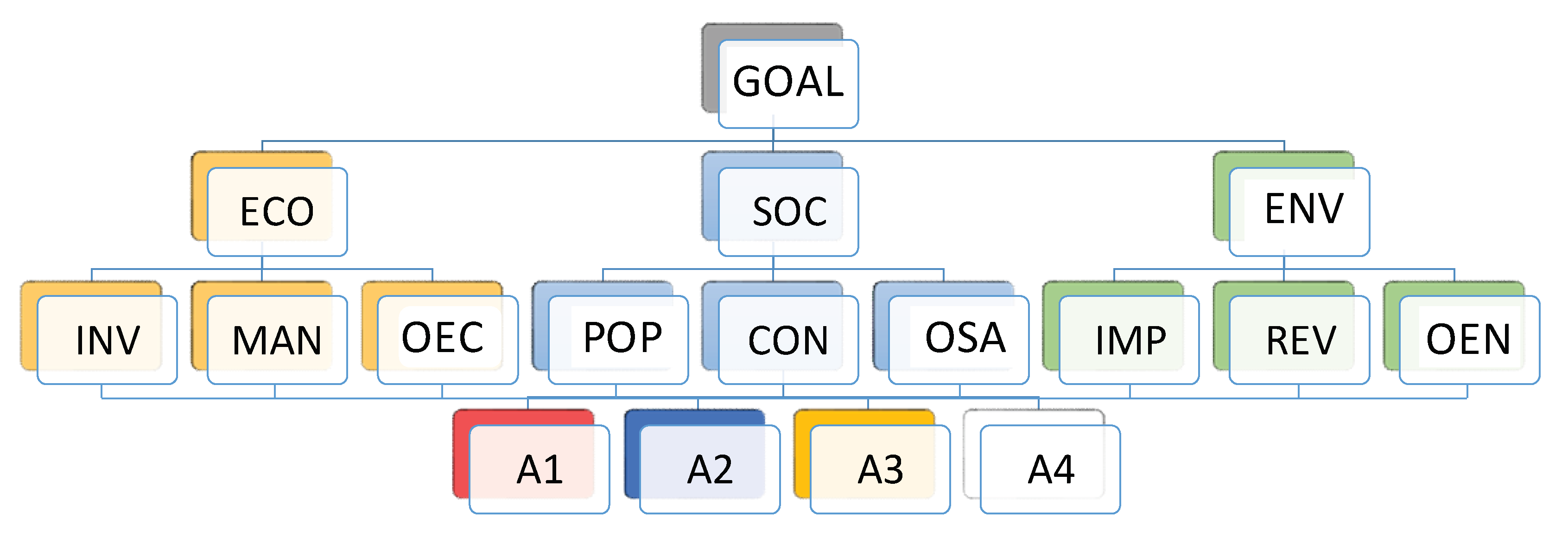
Once the final ${\mathsf{𝒢}}^{(\mathrm{O}\mathrm{c}\mathrm{c}\mathrm{a}\mathrm{m} \mathrm{Window})}$ solution has been obtained, we could act in two different ways: the first one is to select the ${\mathsf{𝒢}}^{(\mathrm{O}\mathrm{p}\mathrm{t}\mathrm{i}\mathrm{m}\mathrm{u}\mathrm{m})}$ partitions with a smaller number of groups included in ${\mathsf{𝒢}}^{(\mathrm{O}\mathrm{c}\mathrm{c}\mathrm{a}\mathrm{m} \mathrm{Window})}$, so that $\left|{\mathsf{𝒢}}^{(\mathrm{O}\mathrm{p}\mathrm{t}\mathrm{i}\mathrm{m}\mathrm{u}\mathrm{m})}\right|={\min }_{\mathsf{𝒢}\in {\mathsf{𝒢}}^{(\mathrm{O}\mathrm{c}\mathrm{c}\mathrm{a}\mathrm{m} \mathrm{Window})}}\left\{\left|\mathsf{𝒢}\right|\right\}$. In this way, as the number of dissenting opinions is lower, it will potentially be easier to reach a broader consensus among the actors in the problem.

However, this solution has the inconvenient of not collecting the uncertainty associated with the model selection process, that is captured by the partitions included in the Occam’s Window ${\mathsf{𝒢}}^{(\mathrm{O}\mathrm{c}\mathrm{c}\mathrm{a}\mathrm{m} \mathrm{Window})}$, which can suggest alternative ways to implement the negotiation process. For this purpose, we propose building a non-directed graph or network $𝒩$ = (V,E). The vertices or nodes would be the set of decision-makers (V = D) and the edges or links (E) between two nodes D and D′ ∈ D would represent the existence of a partition $𝒢$ ∈ ${\mathsf{𝒢}}^{(\mathrm{O}\mathrm{c}\mathrm{c}\mathrm{a}\mathrm{m} \mathrm{Window})}$ that contains a group G ∈ $𝒢$ such that D, D’ ∈ G. In the graph the decision-makers D, D’ ∈ D are closer (further away) if the probability to be classified in the same group is higher (lower). This probability is given by:

$$\mathrm{P}\left(\mathrm{D},\mathrm{D}{}^{\prime } \mathrm{be} \mathrm{classified} \mathrm{in} \mathrm{the} \mathrm{same} \mathrm{group}\right)=\frac{{\displaystyle \sum _{\mathsf{𝒢}\in {\mathsf{𝒢}}^{(\mathrm{O}\mathrm{c}\mathrm{c}\mathrm{a}\mathrm{m}\text{\_}\mathrm{W}\mathrm{i}\mathrm{n}\mathrm{d}\mathrm{o}\mathrm{w})}:\exists \mathrm{G}\in \mathsf{𝒢} \mathrm{with} \mathrm{D},{\mathrm{D}}^{\prime }\in \mathbf{G}}\left[\mathbf{Y}|\mathsf{𝒢}\right]}}{{\displaystyle \sum _{\mathsf{𝒢}\in {\mathsf{𝒢}}^{(\mathrm{O}\mathrm{c}\mathrm{c}\mathrm{a}\mathrm{m}\text{\_}\mathrm{W}\mathrm{i}\mathrm{n}\mathrm{d}\mathrm{o}\mathrm{w})}}\left[\mathbf{Y}|\mathsf{𝒢}\right]}}$$

(10)

In this way, we could see which decision-makers tend to have the same opinions about the alternatives of the decision problem.

4. Case Study

This section illustrates the proposed methodology (AHP-BYC) applied to a case study. This case corresponds to an experience of citizen participation in which various alternatives on the expansion of the tram network in Zaragoza (Spain) were analysed, presented by the main political parties during the electoral campaign of the last municipal elections. The experiment was carried out with 22 students from the Faculty of Economics and Business of the University of Zaragoza in the 2014–2015 academic year and the following four alternatives were considered:

A1:

Build a new tramline

A2:

Use a tram and bus combination called Tran bus

A3:

Use a tram combination with commuter lines

A4:

Do nothing

Figure 2 shows the hierarchy used in the problem, which was comprised four levels (the goal, three criteria, nine attributes and four alternatives).

The three types of criteria used at the highest level of the hierarchy were economic (ECO), social (SOC) and environmental (ENV) ones. We considered three economic sub-criteria namely cost of investment (INV), annual maintenance cost (MAN) and other economic aspects (OEC). In the case of social criteria, the three considered sub-criteria were citizens who access it in less than 3/5 min on foot (POP), comfort, convenience of the alternative: access, facilities, animal services, bikes…(COM) and other social aspects (OSA). Finally, we chose three environmental sub-criteria, namely physical, acoustic, visual impact… (IMP), transport mode reversibility (REV) and other environmental aspects (OEN).

In Section 4.1, we carry out a comparative study of the exhaustive method of reference [3] with the stochastic search method proposed in the work. In Section 4.2, we analyse for the 22 decision-makers of the problem, who provided their pairwise comparison matrices, their opinions for each of the criteria and sub-criteria using the methodology proposed in the work. In both subsections, we take the prior distributions (2) and (3) described in Section 3.2. All the numerical results displayed in the paper were obtained using our own code put together in MATLAB 2019 b.

4.1. Simulation Study

Table 1. Computational times and results of the simulation process.

Criterion	Exhaustive Average CPU Time (Standard Deviation) (K = 11)	Stochastic Search Average CPU Time (Standard Deviation) (K = 11)	% of Simulations Where $𝒢$opt = $𝒢$max (K = 11)	Average Factor Bayes (Standard Deviation) (K = 11)	Stochastic Search Average CPU Time (Standard Deviation) (K = 22)
Environmental	98.68 (0.55)	7.19 (0.20)	93.00%	0.9735 (0.1267)	17.93 (1.50)
Comfort	112.68 (2.10)	9.20 (1.18)	73.00%	0.8762 (0.2583)	80.38 (18.27)
Economic	101.85 (6.81)	7.21 (0.54)	97.00%	1.0000 (0.0000)	15.58 (0.19)
Impact	116.53 (5.73)	8.59 (0.96)	68.00%	0.8271 (0.2826)	51.65 (1.97)
Investment	112.23 (1.17)	7.92 (0.60)	81.00%	0.9162 (0.2033)	29.83 (1.47)
Maintenance	115.58 (6.11)	9.33 (1.59)	61.00%	0.7716 (0.3288)	68.16 (1.25)
Goal	99.59 (1.72)	7.24 (0.25)	100.00%	1.0000 (0.0000)	16.43 (0.28)
Other Environmental Aspects	125.25 (7.29)	9.25 (1.53)	52.00%	0.6996 (0.3576)	74.60 (3.11)
Other Economic Aspects	120.29 (2.00)	8.19 (0.93)	52.00%	0.6772 (0.3782)	50.54 (4.17)
Other Social Aspects	121.41 (4.70)	8.71 (1.06)	69.00%	0.8734 (0.2428)	70.29 (4.20)
Population	131.03 (11.65)	9.01 (1.13)	58.00%	0.7771 (0.3130)	56.67 (10.01)
Reversibility	130.84 (11.03)	10.80 (1.94)	73.00%	0.8649 (0.2693)	88.74 (4.51)
Social	105.16 (2.21)	7.25 (0.37)	93.00%	0.9581 (0.1742)	17.57 (1.86)

compares the results obtained by the exhaustive algorithm of reference [3] and by the stochastic search algorithm (AHP-BYC) proposed in this work. To do this, 100 samples of size 11 were randomly extracted from the set of decision-makers and both algorithms were applied to each of them.

This table shows the average CPU times used by each algorithm and its standard deviation in parentheses, as well as the percentage of simulations in which the stochastic search algorithm located the most probable partition (K = 11), and the average Bayes factor between the most probable partition ${\mathsf{𝒢}}_{\max }$ located by the exhaustive algorithm and the optimal partition ${\mathsf{𝒢}}_{\mathrm{o}\mathrm{p}\mathrm{t}}$ located by the stochastic search algorithm.

A clear reduction in computational time (around 92.5%) is observed in obtaining the optimal partition without producing a significant loss of efficiency. The percentage of simulations in which the most probable partition is found ranges between 52% and 100% and the Bayes factor between the 2 partitions does not drop below 0.65 without the model selected by the algorithm being outside the Occam’s window in any case. Said efficiency is higher in the criteria with 3 elements than in those of 4. Having seen these results, we conclude that the algorithm works well, although we recommend repeating it with several initiations and saving the best solution. This is what we did in the empirical study with the 22 decision-makers where the algorithm was repeated 10 times and the results obtained in each replication were combined, without observing a significant deterioration in computational times (see column Stochastic with K = 22 in Table 1).

4.2. Empirical Study

Table 2. Groups (G_g) and group priorities $\left({\mathrm{w}}_{\mathrm{i}}^{\left(\mathrm{g}\right)}\right)$ corresponding to the goal and criteria.

				GOAL
				Groups	Priorities
					ECO	SOC	ENV
				1, 6, 7, 9, 10, 11, 15, 19, 20	0.6420	0.2481	0.1094
				2, 8, 13	0.4212	0.1145	0.4623
				3	0.0826	0.3497	0.5650
				4, 5, 12, 14, 18, 21, 22	0.2515	0.6673	0.0806
				16, 17	0.1171	0.5791	0.3031
ECONOMIC				SOCIAL				ENVIRONMENTAL
Groups	Priorities			Groups	Priorities			Groups	Priorities
	INV	MAN	OEC		POP	COM	OSA		IMP	REV	OEN
1, 8, 11, 22	0.5652	0.1150	0.3182	1, 2, 3, 5, 6, 7, 10, 16, 17	0.6503	0.2274	0.1217	1,11	0.5423	0.2278	0.2292
2,7, 10, 13, 15, 19, 20, 21	0.6296	0.2435	0.1267	4, 14	0.0858	0.6437	0.2666	2, 3, 6, 13, 15, 16, 18, 20, 22	0.6568	0.2266	0.1160
3, 4, 5, 6, 9, 12, 14, 16, 17	0.2626	0.6441	0.0929	8, 11, 13, 18, 20, 21	0.6344	0.1239	0.2410	4, 5	0.1347	0.3111	0.5533
18	0.1164	0.2764	0.6039	9, 12, 15, 19	0.2237	0.6460	0.1290	7, 12, 19, 21	0.2578	0.6333	0.1078
				22	0.2419	0.1095	0.6438	8, 9, 10, 14, 17	0.4649	0.1137	0.4186

shows the composition of the groups corresponding to the optimal partition obtained using the AHP-BYC methodology, as well as the posterior medians of the priorities of each group estimated for each of the alternatives. The same information is provided in

Table 3. Groups (G_g) and group priorities $\left({\mathrm{w}}_{\mathrm{i}}^{\left(\mathrm{g}\right)}\right)$ corresponding to the economic sub-criteria.

INVESTMENT					MAINTENANCE					OTHER ECONOMIC ASPECTS
Groups	Priorities				Groups	Priorities				Groups	Priorities
	A1	A2	A3	A4		A1	A2	A3	A4		A1	A2	A3	A4
1, 2, 3, 7, 12, 15, 16, 17, 19, 20, 21, 22	0.0626	0.2573	0.1197	0.5597	1, 16, 19	0.1898	0.054	0.1615	0.5891	1, 11	0.1562	0.5718	0.1398	0.127
4, 10	0.6129	0.1602	0.0925	0.1318	2, 6, 7, 12, 17, 20	0.2295	0.1238	0.0788	0.5657	2, 7, 16	0.2280	0.1829	0.1607	0.4255
5, 6	0.2979	0.1300	0.0639	0.5032	3	0.1247	0.5702	0.0655	0.2339	3	0.1163	0.5631	0.0658	0.2479
8, 18	0.1132	0.2716	0.0512	0.5609	4, 10	0.5738	0.2082	0.1151	0.0985	4, 10, 20	0.5589	0.1828	0.1517	0.1042
9, 14	0.1427	0.1128	0.6566	0.078	5, 8, 15, 18, 22	0.0878	0.2337	0.0753	0.6014	5, 6, 8, 17, 19	0.1366	0.1800	0.0532	0.6287
11	0.1225	0.4685	0.2744	0.1289	9, 14	0.2169	0.1261	0.5848	0.0701	9, 14, 18, 22	0.1560	0.1212	0.6302	0.0882
13	0.1014	0.1672	0.2855	0.4422	11	0.2613	0.446	0.1424	0.1483	12, 13, 15, 21	0.0663	0.1773	0.1811	0.5734
					13, 21	0.1145	0.1233	0.2621	0.4969

,

Table 4. Groups (G_g) and group priorities $\left({\mathrm{w}}_{\mathrm{i}}^{\left(\mathrm{g}\right)}\right)$ corresponding to the social sub-criteria.

POPULATION					COMFORT					OTHER SOCIAL ASPECTS
Groups	Priorities				Groups	Priorities				Groups	Priorities
	A1	A2	A3	A4		A1	A2	A3	A4		A1	A2	A3	A4
1, 7, 18, 21	0.1432	0.3243	0.466	0.0615	1, 11, 19	0.2409	0.4903	0.1865	0.0758	1, 11	0.1139	0.6195	0.1401	0.1182
2, 14	0.4726	0.1551	0.2581	0.1094	2, 21	0.4476	0.1967	0.2676	0.0858	2, 4, 10, 13, 15, 16, 17, 19, 20	0.4938	0.2627	0.1703	0.0715
3, 6, 8, 9	0.1269	0.3035	0.0716	0.4931	3, 9	0.0938	0.4797	0.0864	0.3337	3, 5, 6, 8, 9	0.1428	0.3025	0.0820	0.4691
4, 5, 10, 12, 15, 16	0.5502	0.2368	0.1074	0.1041	4, 5, 10	0.5373	0.2482	0.0884	0.1247	7, 21, 22	0.2144	0.2916	0.4194	0.0722
11	0.2248	0.4525	0.1446	0.1754	6, 8	0.1856	0.1924	0.0669	0.5498	12, 18	0.2998	0.0972	0.5464	0.0531
13, 17, 19, 20, 22	0.4269	0.3742	0.1479	0.0486	7, 13, 15, 16, 17, 20, 22	0.5012	0.2781	0.1607	0.0594	14	0.1141	0.0867	0.5519	0.2400
					12, 14	0.2418	0.116	0.5813	0.0582
					18	0.2500	0.2500	0.2500	0.2500

and

Table 5. Groups (G_g) and group priorities $\left({\mathrm{w}}_{\mathrm{i}}^{\left(\mathrm{g}\right)}\right)$ corresponding to the environmental sub-criteria.

IMPACT					REVERSIBILITY					OTHER ENVIRONMENTAL ASPECTS
Groups	Priorities				Groups	Priorities				Groups	Priorities
	A1	A2	A3	A4		A1	A2	A3	A4		A1	A2	A3	A4
1	0.0773	0.5945	0.1991	0.1274	1	0.0579	0.6617	0.2061	0.0679	1	0.0680	0.6584	0.1869	0.0807
2, 7	0.1802	0.0951	0.2849	0.4369	2, 3, 7, 9, 12, 17, 21, 22	0.0722	0.3139	0.1298	0.4831	2, 6, 16, 17	0.2396	0.1144	0.0735	0.5705
3, 5, 8, 18, 20	0.1137	0.3355	0.0772	0.4728	4, 11	0.2668	0.4765	0.1374	0.1173	3, 13, 15, 19, 21, 22	0.0764	0.1791	0.1584	0.584
4, 9	0.3354	0.0967	0.4601	0.1027	5	0.3090	0.2674	0.1559	0.2656	4, 11	0.2549	0.4865	0.1370	0.1195
6, 17	0.2783	0.1141	0.0799	0.5253	6, 8, 16, 18	0.1275	0.2291	0.0632	0.5767	5, 8	0.1192	0.2793	0.0711	0.5278
10, 16	0.5395	0.2163	0.1176	0.1221	10, 20	0.5753	0.2007	0.1253	0.0948	7, 12, 18	0.2329	0.0666	0.1686	0.5282
11	0.2387	0.5230	0.1150	0.1208	13, 14, 15, 19	0.0854	0.1145	0.2095	0.5874	9, 10, 20	0.4846	0.2108	0.1770	0.1180
12, 13, 15, 19, 21, 22	0.0572	0.2056	0.1167	0.6190						14	0.1006	0.1461	0.5129	0.2358
14	0.0945	0.1985	0.5457	0.1565

for the nine sub-criteria.

Likewise, Figure 3, Figure 4, Figure 5 and Figure 6 show the graphs $𝒩$ obtained by applying the procedure described in Section 3.2.4 to the goal and each criterion/sub-criterion represented in Figure 2. These graphs were obtained using the igraph package of the statistical program R. The different groups are indicated by surrounding the corresponding decision-makers with coloured lines. The preferred rankings of each group are enclosed in light blue rectangles. The preference structures of each group are constructed from their gamma distributions and a distinction is made between strict preference (>) and non-strict preference (≥) depending on the appearance of one or more preference structures with a posteriori probability greater than or equal to 0.2.

Thus, for example, if we consider the Goal, we can see the existence of five groups: G₁ = {D₁, D₆, D₇, D₉, D₁₀, D₁₁, D₁₅, D₁₉, D₂₀}, G₂ = {D₂, D₈, D₁₃}, G₃ = {D₃}, G₄ = {D₄, D₅, D₁₂, D₁₄, D₁₈, D₂₁, D₂₂} and G₅ = {D₁₆, D₁₇}. The posterior median priorities of G₁ are ${\mathrm{w}}_{\mathrm{E}\mathrm{C}\mathrm{O}}^{\left(1\right)}$= 0.6420, ${\mathrm{w}}_{\mathrm{S}\mathrm{O}\mathrm{C}}^{\left(1\right)}$ = 0.2481, ${\mathrm{w}}_{\mathrm{E}\mathrm{N}\mathrm{V}}^{\left(1\right)}$ = 0.1094 (Table 2) and the most probable preference structure is ECO > SOC > ENV (Figure 3). This structure reflects, on the one hand, that said group places the Economic criterion as the most preferred, followed by the Social criterion and the Environmental criterion as the least preferred. Some of these preferences are not strict. Therefore, for instance, group G₂ has ENV ≥ ECO > SOC as the most probable preference structure, because the most preferred structures are ENV > ECO > SOC and ECO > ENV > SOC with posterior probabilities 0.5938 and 0.4059, respectively. This reflects that the group priorities ${\mathrm{w}}_{\mathrm{E}\mathrm{C}\mathrm{O}}^{\left(2\right)}$ = 0.4212 and ${\mathrm{w}}_{\mathrm{E}\mathrm{N}\mathrm{V}}^{\left(2\right)}$= 0.4623 are similar (see Table 2).

We can therefore observe that most of the groups relegate the environmental criteria to third place, with two majority groups of 9 decision-makers clearly separated in the Goal graph: G₁ on the one hand, and G₄ ∪ G₅ on the other hand, that place the economic or social criteria as the most important ones, respectively. In addition, the graph of the Goal highlights that decision-makers who support economic criterion as the most preferred are more homogeneous in their opinions about the rankings of compared criteria than those who support social criterion, and these differ in their opinion about the importance of the economic and environmental criteria (see Figure 3).

Regarding the economic sub-criteria (see Figure 4 and Table 3), the most preferred sub-criterion is investment (12 decision-makers) followed by the maintenance sub-criteria (9 decision-makers). In the case of the social sub-criteria (see Figure 5 and Table 4), the most preferred sub-criterion is population (15 decision-makers) followed by the comfort sub-criterion (6 decision-makers). Finally, among the environmental sub-criteria (see Figure 6 and Table 5), the most preferred sub-criterion is environmental impact (16 decision-makers), followed by the reversibility criterion (4 decision-makers).

If we analyse each economic sub-criterion (Table 3 and Figure 4), we see that, in general, the most supported alternative is A₄ (17 decision-makers in the investment criterion, 18 decision-makers in the maintenance and 12 decision-makers in other economic aspects. For the rest of the alternatives, the support shown for alternative A₂ in the investment sub-criterion stands out and tends to occupy the first or second place in the opinion of 17 decision-makers.

With respect to each social sub-criterion (Table 4 and Figure 5), we can see that the alternative most supported by the 3 sub-criteria is A₁ (14 decision-makers in population, 12 decision-makers in comfort and 9 decision-makers in other social aspects). For the rest of the alternatives, the support shown for alternative A₂ to occupy the first or second place (19 decision-makers in population, 17 in comfort and 13 in other social aspects) stands out.

Finally, regarding each environmental criterion (Table 5 and Figure 6) we can see that A₄ is the most supported alternative by the 3 sub-criteria (15 decision-makers in environmental impact, 16 decision-makers in reversibility and 15 decision-makers in other environmental aspects). For the rest of the alternatives, it highlights the support shown for alternative A₂ to occupy the first or second place (16 decision-makers in impact, 16 in reversibility and 14 in other environmental aspects).

In short: the most preferred criteria are the economic and social ones, which are supported by the same number (9) of decision-makers. If we consider the sub-criteria, it is observed that alternative A₄ (do nothing) is supported mostly by decision-makers in the economic and environmental sub-criteria, while alternative A₁ (build a new tram line) is supported by the social sub-criteria. Therefore, the negotiation should be considered at the level of economic and environmental criteria, on one hand, and social criteria, on the other, deciding which of them is given more priority. Based on this priority, the chosen alternative would be to build the new tram line if social criteria are given higher priority or to do nothing, if economic and environmental criteria are given higher priority. On the other hand, analysing the graphs of the sub criteria, another alternative negotiation line can be appreciated. This line would propose the alternative A₂ (use a tram and bus combination called Tran bus) as a final solution since a large number of decision-makers place it in the first or second place of their preferences in all the sub-criteria.

5. Conclusions

The representativeness of the collective position in multiactor decision making, and the identification of homogeneous groups of decision-makers with discrepant priorities between the groups, are two problems that are widely discussed in general scientific literature due to their interest. Unfortunately, in the context of AHP, these issues have received very little attention, particularly in the case of stochastic AHP.

The specific characteristics of the AHP, especially the uncertainty inherent in the assessment of intangible aspects and the acceptable inconsistency allowed when incorporating the judgments of the decision-maker, recommend the analysis of these two problems following a stochastic (Bayesian in this case) approach. Consistent with this fact, the paper proposes a new stochastic search algorithm (AHP-BYC) for the identification of homogeneous groups of actors. The algorithm is based on Bayesian tools for model comparison and selection and uses the Bayes factor as the model comparison tool. The underlying clustering process combines randomly classical divisive and agglomerative steps with a probabilistic evaluation of the quality of the explored partitions, which provides a more efficient and rigorous classification procedure. Some of these steps are specific to the AHP context, which makes the algorithm very efficient with significantly lower computational times.

As a result, the algorithm calculates the Occam’s window, which contains the partitions that describe, in a parsimonious way, the different preferences of the actors involved in the resolution of the problem. This algorithm is complemented with graphic tools based on the use of networks to analyze the similarities of the decision-maker’s preferences and to facilitate subsequent negotiation processes.

The methodological novelty of the AHP-BYC proposal is associated with the joint consideration of the following aspects: (i) a Bayesian approach is followed in the treatment of uncertainty; (ii) Bayesian tools for model comparison and selection are used; (iii) the Bayes factor is used to measure the similarities between partitions; (iv) individual AHP preference structures are considered to formulate more efficient search procedures in the partition space; (v) determination of partitions that describes, in a parsimonious way, the preferences of the actors; (vi) preparation of graphic tools to analyze the similarities of these preferences which can be used to carry out the negotiation processes and, finally, (vii) use of the characteristics and properties of the AHP approach to reach more representative positions, that is to say, positions supported by a greater number of individuals.

An illustrative application of the algorithm to an experience of citizen participation in which various alternatives on the expansion of the tram network in Zaragoza (Spain) is carried out. The most supported alternatives and criteria are identified, and some negotiation recommendations are provided.

With regards to the limitations of this new methodological proposal, the following points can be considered: the case of incomplete information (PCMs); the theoretical background necessary to implement the approach; and the difficulty in comparing it with other Bayesian approaches.

As future research lines, we contemplate the incorporation of additional movements in the exploration of the partition space, the construction of new stochastic indicators to compare the goodness of the different (Bayesian) partitions, the improvement of the efficiency of the algorithm, and the extension to hierarchies of the previously analyzed local case (one criterion). Another future line would be the design of algorithms that use computationally more simple cluster techniques which have shown great efficiency in the analysis of large databases (non-hierarchical partitioning methods such as k-means or decision trees, …). These algorithms would be combined with the use of statistical models to evaluate the quality of the selected partitions. Finally, it would also be interesting to compare the efficiency of these algorithms with the one proposed here.

References

1. Saaty, T.L. The Analytic Hierarchy Process; Mc Graw-Hill: New York, NY, USA, 1980. [Google Scholar]
2. Escobar, M.; Moreno-Jiménez, J.M. Aggregation of Individual Preference Structures in AHP-Group Decision Making. Group Decis. Negotiat. 2007, 16, 287–301. [Google Scholar] [CrossRef]
3. Altuzarra, A.; Gargallo, P.; Moreno-Jiménez, J.M.; Salvador, M. Homogeneous Groups of Actors in an AHP-Local Decision Making Context: A Bayesian Analysis. Mathematics 2019, 7, 294. [Google Scholar] [CrossRef] [Green Version]
4. Altuzarra, A.; Moreno-Jiménez, J.M.; Salvador, M. Consensus Building in AHP-Group Decision Making: A Bayesian Approach. Oper. Res. 2010, 58, 1755–1773. [Google Scholar] [CrossRef]
5. Moreno-Jiménez, J.M.; Salvador, M.; Gargallo, P.; Altuzarra, A. Systemic decision making in AHP: A Bayesian approach. Ann. Oper. Res. 2016, 245, 261–284. [Google Scholar] [CrossRef]
6. Zhou, M.; Hu, M.; Chen, Y.-W.; Cheng, B.-Y.; Wu, J.; Herrera-Viedma, E. Towards achieving consistent opinion fusion in group decision making with complete distributed preference relations. Knowledge-Based Systems. 2021, 236, 107740. [Google Scholar] [CrossRef]
7. Madigan, D.; Raftery, A.E. Model Selection and Accounting for Model Uncertainty in Graphical Models Using Occam’s Window. J. Am. Stat. Assoc. 1994, 89, 1535–1546. [Google Scholar] [CrossRef]
8. Clyde, M.; Gosh, J. Finite Population Estimators in Stochastic Search Variable Selection. Biometrika 2012, 99, 981–988. [Google Scholar] [CrossRef] [Green Version]
9. Lamnisos, D.; Griffin, J.E.; Steel, M.F.J. Adaptive Monte Carlo for Bayesian Variable Selection in Regression Models. J. Comput. Graph. Stat. 2013, 22, 729–748. [Google Scholar] [CrossRef]
10. Lyiang, F.; Paulo, R.; Molina, G.; Clyde, M.A.; Berger, J.O. Mixtures of g Priors for Bayesian Variable Selection. J. Am. Stat. Assoc. 2008, 103, 410–423. [Google Scholar] [CrossRef]
11. Nott, D.J.; Kohn, R. Adaptive sampling for Bayesian variable selection. Biometrika 2005, 92, 747–763. [Google Scholar] [CrossRef]
12. Steel, M.F.J. Model Averaging and Its Use in Economics. J. Econ. Lit. 2020, 58, 644–719. [Google Scholar] [CrossRef]
13. Kass, R.E.; Raftery, A.E. Bayes factors. J. Am. Stat. Assoc. 1995, 90, 773–795. [Google Scholar] [CrossRef]
14. Crawford, G.; Williams, C. A Note on the Analysis of Subjective Judgment Matrices. J. Math. Psychol. 1985, 29, 387–405. [Google Scholar] [CrossRef]
15. Aguarón, J.; Moreno-Jiménez, J.M. The geometric consistency index: Approximate thresholds. Eur. J. Oper. Res. 2003, 147, 137–145. [Google Scholar] [CrossRef]
16. Altuzarra, A.; Moreno-Jiménez, J.M.; Salvador, M. A Bayesian priorization procedure for AHP-group decision making. Eur. J. Oper. Res. 2007, 182, 367–382. [Google Scholar] [CrossRef]
17. Moreno-Jiménez, J.M.; Aguarón, J.; Escobar, M.T. The core of consistency in AHP-group decision making. Group Decis. Negotiat. 2008, 17, 249–265. [Google Scholar] [CrossRef]
18. Escobar, M.T.; Aguarón, J.; Moreno-Jiménez, J.M. Some extensions of the precise consistency consensus matrix. Decis. Support Syst. 2015, 74, 67–77. [Google Scholar] [CrossRef]
19. Ramanathan, R.; Ganesh, L.S. Group preference aggregation methods employed in AHP: An evaluation and intrinsic process for deriving members’ weightages. Eur. J. Oper. Res. 1994, 79, 249–265. [Google Scholar] [CrossRef]
20. Forman, E.; Peniwati, K. Aggregating individual judgements and priorities with the analytic hierarchy process. Eur. J. Oper. Res. 1998, 108, 165–169. [Google Scholar] [CrossRef]
21. Aguarón, J.; Escobar, M.T.; Moreno-Jiménez, J.M.; Turón, A. Geometric Compatibility Indexes in a Local AHP-Group Decision Making Context: A Framework for Reducing Incompatibility. Mathematics 2022, 10, 278. [Google Scholar] [CrossRef]
22. Akogul, S.; Erisoglu, M. An Approach for Determining the Number of Clusters in a Model-Based Cluster Analysis. Entropy 2017, 19, 452. [Google Scholar] [CrossRef] [Green Version]
23. Benítez, J.; Carpitella, S.; Certa, A.; Ilaya-Ayza, A.E.; Izquierdo, J. Consistent clustering of entries in large pairwise comparison matrices. J. Comput. Appl. Math. 2018, 343, 98–112. [Google Scholar] [CrossRef]
24. Meixner, O.; Haas, R.; Pöchtrager, S. AHP Group Decision Making and Clustering. In Proceedings of the International Symposium on the Analytic Hierarchy Process (ISAHP) Multi-Criteria Decision Making, London, UK, 4–8 August 2016; Available online: https://www.researchgate.net/publication/327733984_AHP_GROUP_DECISION_MAKING_AND_CLUSTERING (accessed on 21 January 2022). [CrossRef]
25. Song, Y.; Hu, Y. Group Decision-Making Method in the Field of Coal Mine Safety Management Based on AHP with Clustering. In Proceedings of the 6th International ISCRAM Conference, Gothenburg, Sweden, 10–13 May 2009. [Google Scholar]
Figure 1. Steps of the proposed methodology (AHP-BYC).
Mathematics 10 00519 g001
Figure 2. Hierarchy of criteria and sub-criteria used in the case study.
Mathematics 10 00519 g002
Figure 3. Graphs of decision-makers corresponding to the goal and the criteria of the problem.
Mathematics 10 00519 g003
Figure 4. Graphs of decision-makers for the economic criterion and its sub-criteria.
Mathematics 10 00519 g004
Figure 5. Graphs of decision-makers for the social criterion and its sub-criteria.
Mathematics 10 00519 g005
Figure 6. Graphs of decision-makers for the environmental criterion and its sub-criteria.
Mathematics 10 00519 g006