A Methodology for Estimating Vehicle Route Choice from Sparse Flow Measurements in a Traffic Network

Abstract

While traffic speed data and travel time estimates are increasingly more available from commercial vendors, they are not sufficient for proper management and performance evaluation of transportation networks. Effective traffic control and demand management requires information about volumes, which is provided by fixed location sensors, such as loop detectors or cameras, and those are sparse. This paper proposes a method for estimating route choice using sparse flow measurements and estimated speed on the road network based on compressed sensing technology widely used in image processing, where from a handful of scattered pixels, a full image is recovered. What is known includes flows at origins and at selected links of the road network, where the detection is present; speed estimates are available for all network links. We find coefficients that split origin flows among routes starting at those origins. The advantage of the proposed methodology is that it does not rely on simulation that is prone to calibration errors but only on measured data. We also show how vehicle flows can be estimated at links with no detection, which enables computing performance measures for road networks lacking complete sensor coverage. Finally, we propose a method for selecting plausible routes between origins and destinations.

1. Introduction

One of the main challenges of urban traffic management is the shortage of traffic volume measurements. While traffic speed data and travel time estimates are increasingly more available from commercial vendors, they do not provide information about traffic volumes needed for effective traffic control, demand management and performance evaluation. Traffic volumes are measured by static sensors (loop detectors, magnetic sensors, radars and cameras) mounted into the roadside infrastructure, and those are sparse. What would help in this situation is the knowledge of the origin-destination (O-D) matrix and information about route assignment.

The difficulty of O-D estimation is in the fact that it is an underdetermined (allowing multiple solutions) problem [1,2,3,4]. Traditionally, there are three main approaches to the O-D estimation [5]: the first one assumes that trips follow a gravity type pattern and the problem is reduced to calibrating the parameters of such a model from the observed counts [6]; the second approach estimates the O-D matrix by using user equilibrium traffic assignment based on Wardrop’s first principle [7,8]; and the third is an entropy maximising approach, in which the most likely trip matrix compatible with the observed flows is sought [1].

To make use of the first approach, one has to deal with land use data, attraction potential of zones and detailed activity models—e.g., [9,10,11,12,13]. The combination of the second and third approaches entails the use of various traffic data sources and the invocation of traffic assignment, which employs one or another traffic model. This topic was extensively studied throughout the years—e.g., [1,2,3,14,15,16,17,18,19,20,21,22]. The literature survey on the second and third approaches is given in [23]. Generally, the methodology can be summarized in the following iterative 5-step process requiring simulation:

• An a priori O-D matrix is assumed that may be an old O-D matrix or a matrix generated from surveys.
• The flows in the O-D matrix are mapped to the network using traffic assignment algorithms.
• Assigned flows are compared with measured flows.
• The a priori O-D matrix is adjusted to match the measured flows. For this, different solution approaches can be used.
• The adjusted O-D matrix is used again in step 1 until convergence of the assigned and measured flows and/or the a priori and estimated matrix.

This paper proposes a method of estimating route choice using sparse flow measurements and estimated speed on the road network. The flows at origins and at selected links of the road network are known, where the detection is present; speed estimates are available for all network links. We find coefficients that split origin flows among routes starting at those origins. The problem is cast as a non-negative least squares problem with sparsity constraints. To our knowledge, the proposed approach is new, and it promises efficient technology for road network performance evaluation and traffic flow estimation required for traffic control and demand management.

The rest of the paper is organized as follows. Section 2 contains the problem formulation. The algorithm for computing split coefficients is presented in Section 3. Section 4 describes approaches to the initial selection of plausible routes. Finally, Section 5 concludes the paper.

2. Problem Statement

The road network consists of directed links and nodes: Links represent stretches of roads with specified direction of travel, and nodes connect the links. A node with no input links is called origin (O), and a node with no output links is called destination (D). For a given urban area, transportation planners come up with the four-step demand model [24], where the area is divided into zones resulting from land use analysis and forecasting. Thus, for Z zones, we obtain $(Z^2-Z)$ O-D pairs (each zone is connected to other zones but not itself).

We assume that for every O-D pair, we know all plausible routes. Thus, we have the list of all routes in a given road network. Furthermore, we assume that at each time, we have an estimate of speed for all the links in the road network. (Speed estimates may come from GPS probes and are provided by commercial vendors, such as HERE Traffic).

Suppose for a moment that vehicle flows at every origin, and vehicle flows at some links that belong to one or more routes in the road network are known: these flows are measured by inductive loops, magnetic sensors, radars or cameras.

Throughout the paper, we shall use the notation presented in

Table 1. Notation.

Parameter	Description
$\mathcal{O}$	Set of origins. Its size $\left|\mathcal{O}\right|=Z$, the number of zones.
$o\in \mathcal{O}$	Origin.
$\mathcal{R}$	Set of all routes.
${\mathcal{R}}^o\subset \mathcal{R}$	Subset of routes starting at origin $o\in \mathcal{O}$.
$r\in \mathcal{R}$	Route.
$r^o\in {\mathcal{R}}^o$	Route starting at origin $o\in \mathcal{O}$.
$\mathcal{L}$	Set of links that belong to one or more routes in $\mathcal{R}$.
$\tilde{\mathcal{L}}\subset \mathcal{L}$	Subset of route links with flow measurements.
$|\tilde{\mathcal{L}}|$ ($\left|\mathcal{L}\right|$)	Number of links in the set.
$l\in \tilde{\mathcal{L}}$ ($l\in \mathcal{L}$)	Link.
$\left|l\right|$	Link length.
${\mathcal{R}}_l\subset \mathcal{R}$	Subset of routes containing link $l\in \mathcal{L}$.
$|{\mathcal{R}}_l|$ ($|{\mathcal{R}}^o|$ or $\left|\mathcal{R}\right|$)	Number of routes in the set.
$r_l\in {\mathcal{R}}_l$	Route containing link $l\in \mathcal{L}$.
$f^o$	Flow (vehicle count) measured at origin $o\in \mathcal{O}$.
$f_l$	Flow (vehicle count) measured at link $l\in \tilde{\mathcal{L}}$.
${\alpha }_{r^o}\in [0,1]$	Portion of flow $f^o$ directed to route $r^o$. ${\sum }_{r^o\in {\mathcal{R}}^o}{\alpha }_{r^o}=1$.
${\beta }_l^o\in [0,1]$	Portion of flow $f_l$, contributed by vehicles from origin o. ${\sum }_{o\in \mathcal{O}}{\beta }_l^o=1$.
$v^l$	Speed measured or estimated at link $l\in \mathcal{L}$.

.

Problem 1.

For each origin $o\in \mathcal{O}$, find coefficients ${\alpha }_{r^o}$ splitting the origin flow between routes $r^o\in {\mathcal{R}}^o$. The dual problem formulation is as follows: for each link $l\in \tilde{\mathcal{L}}$ with known flow $f_l$, find which portion ${\beta }_l^o$ of this flow is contributed by which origin o.

This is a compressed sensing problem [25] applied to transportation. Compressed sensing is a signal processing technique for efficiently acquiring and reconstructing a signal by finding solutions to underdetermined linear systems. Taking advantage of the signal’s sparseness in some domain, it allows the entire signal to be determined from relatively few measurements. One prominent application of compressed sensing is magnetic resonance tomography.

By solving this problem, we achieve the following:

1. 

Method of computing how much each origin contributes to given bottleneck activation and resulting congestion;

2. 

Method of computing flows on links without direct flow measurements—all without simulation;

3. 

Method of determining the value of road sensor measurements (some may be redundant) and indicating places that need detection.

3. Computing Split Coefficients

We shall consider two cases: (1) static case—vehicles are counted at origins and at links with detection only once; and (2) case with traffic dynamics—when vehicles from origins arrive at links with detection after some travel delays. The first case is relatively easy and explains the idea. Its practical application is in sensor placement in which links should detectors be installed to enable the unique solution of the problem described in the previous section. The second case requires speed estimates on all route links of the road network. These two cases are described next.

3.1. Static Case

This case describes a hypothetical situation when $f^o$ vehicles leave each origin $o\in \mathcal{O}$, and then $f_l$ vehicles are counted at each link $l\in \tilde{\mathcal{L}}$. All happens “in one shot” without taking into account travel delays or traffic conditions. Matching the origin flows $f^o$ with those measured at links, $f_l$, we arrive at the following linear equations:

$$\sum _{o\in \mathcal{O}}{f}^o\sum _{r^o\in {\mathcal{R}}_l}{\alpha }_{r^o}=f_l,l=1,\dots ,\left|\tilde{\mathcal{L}}\right|,$$

(1)

where $\left\{{\alpha }_{r^o}\right\}$ is unknown and should be found. Here, the notation $r^o\in {\mathcal{R}}_l$ means the following: routes originating at the origin o and passing through link l. Additional constraints apply to split coefficients (see Table 1):

$$\begin{array}{ccc}& & \sum _{r^o\in {\mathcal{R}}^o}{\alpha }_{r^o}=1,\forall o\in \mathcal{O};\hfill \end{array}$$

(2)

$$\begin{array}{ccc}& & {\alpha }_{r^o}\ge 0,r^o\in {\mathcal{R}}^o,\forall o\in \mathcal{O}.\hfill \end{array}$$

(3)

Converting Equations (1) and (2) to matrix form, we obtain the following:

$$\left[\begin{array}{ccccc}{\Phi }_{|\tilde{\mathcal{L}}|\times |{\mathcal{R}}^1|}^1& \cdots & {\Phi }_{|\tilde{\mathcal{L}}|\times |{\mathcal{R}}^o|}^o& \cdots & {\Phi }_{|\tilde{\mathcal{L}}|\times |{\mathcal{R}}^{\left|\mathcal{O}\right|}|}^{\left|\mathcal{O}\right|}\\ {\mathbf{1}}_{1\times |{\mathcal{R}}^1|}& \cdots & {\mathbf{0}}_{1\times |{\mathcal{R}}^o|}& \cdots & {\mathbf{0}}_{1\times |{\mathcal{R}}^{\left|\mathcal{O}\right|}|}\\ ⋮& \ddots & ⋮& ⋮& ⋮\\ {\mathbf{0}}_{1\times |{\mathcal{R}}^1|}& \cdots & {\mathbf{1}}_{1\times |{\mathcal{R}}^o|}& \cdots & {\mathbf{0}}_{1\times |{\mathcal{R}}^{\left|\mathcal{O}\right|}|}\\ ⋮& ⋮& ⋮& \ddots & ⋮\\ {\mathbf{0}}_{1\times |{\mathcal{R}}^1|}& \cdots & {\mathbf{0}}_{1\times |{\mathcal{R}}^o|}& \cdots & {\mathbf{1}}_{1\times |{\mathcal{R}}^{\left|\mathcal{O}\right|}|}\end{array}\right]\left[\begin{array}{c}{\mathit{\alpha }}_{|{\mathcal{R}}^1|\times 1}^1\\ ⋮\\ {\mathit{\alpha }}_{|{\mathcal{R}}^o|\times 1}^o\\ ⋮\\ {\mathit{\alpha }}_{|{\mathcal{R}}^{\left|\mathcal{O}\right|}|\times 1}^{\left|\mathcal{O}\right|}\end{array}\right]=\left[\begin{array}{c}{f}_1\\ ⋮\\ f_l\\ ⋮\\ f_{\left|\mathcal{L}\right|}\\ {\mathbf{1}}_{\left|\mathcal{O}\right|\times 1}\end{array}\right],$$

(4a)

where subscripts denote matrix dimensions; $\mathbf{0}$ is a matrix with all elements equal to 0; $\mathbf{1}$ is a matrix with all elements equal to 1; ${\mathit{\alpha }}_{|{\mathcal{R}}^o|\times 1}^o={\left[{\alpha }_{1^o}\cdots {\alpha }_{r^o}\cdots {\alpha }_{|{\mathcal{R}}^o{|}^o}\right]}^T$; and

$${\Phi }_{|\tilde{\mathcal{L}}|\times |{\mathcal{R}}^o|}^o={\left\{{\varphi }_{l{r}^o}\right\}}_{r^o=1,\cdots ,\left|{\mathcal{R}}^o\right|}^{l=1,\cdots ,|\tilde{\mathcal{L}}|},\mathrm{with} {\varphi }_{l{r}^o}=\left\{\begin{array}{cc}{f}^o,\hfill & \mathrm{if} \mathrm{route} r^o\in {\mathcal{R}}_l,\hfill \\ 0,\hfill & \mathrm{otherwise}.\hfill \end{array}\right.$$

In Equation (4a), the parts above the horizontal lines corresponds to Equation (1), and the parts below the horizontal lines correspond to Equation (2).

To simplify the notation, we rewrite Equation (4a) as follows.

$$\mathbf{\Phi }\mathit{\alpha }=\mathit{f}.$$

(4b)

Due to the nonnegativity constraints (3), the system of linear Equation (4b) cannot be solved directly but must be cast as a convex optimization problem, namely, as nonnegative least squares.

$$\underset{\alpha \ge \mathbf{0}}{min}{\parallel \mathbf{\Phi }\mathit{\alpha }-\mathit{f}\parallel }_2^2.$$

(5)

This problem always has a solution. If the original system of equations and inequalities (1)–(3) has a unique solution, solving problem (5) produces exactly that. In case the system (1)–(3) is overdetermined and inconsistent—that is, it has no solution—the solution of problem (5), ${\mathit{\alpha }}^{*}\ge \mathbf{0}$, yields the smallest in Euclidean norm sense perturbation to $\mathit{f}$, $\mathbf{\delta }\mathit{f}$, such that $\mathbf{\Phi }{\mathit{\alpha }}^{*}=\mathit{f}+\mathbf{\delta }\mathit{f}$.

The most interesting case is when the original system (1)–(3) and problem (5), are underdetermined, allowing infinite number of solutions. It is also the most common practical situation, when there are many more routes in the network than functional sensors. How do we determine the solution then? The first obvious suggestion is as follows: install more flow measuring sensors. The links for new sensor installation should be picked so that new rows in matrix $\mathbf{\Phi }$ would be linearly independent of the existing ones reducing the dimension of matrix kernel. Unfortunately, even with new sensors in place, the system will likely remain underdetermined, as in the real world there are typically many more possible routes between zones than sensors.

The general approach to regularization of underdefined problem (5) is to add ${\ell }_1$ or ${\ell }_2$ norm penalty to the objective function.

$$\underset{\alpha \ge 0}{min}{\parallel \mathbf{\Phi }\mathit{\alpha }-\mathit{f}\parallel }_2^2+{\parallel \mathit{\alpha }\parallel }_p,p=1 \mathrm{or} 2.$$

(6)

Regularization with ${\ell }_2$ norm ($p=2$) is called Tikhonov regularization [26], also known as ridge regression. Tikhonov regularization promotes assigning values to components of vector $\mathit{\alpha }$ as uniformly as possible.

Regularization with ${\ell }_1$ norm ($p=1$) is referred to as LASSO (Least Absolute Shrinkage and Selection Operator). LASSO regularization is generally used to promote sparse solutions. For our problem, however, it does not help, because the ${\ell }_1$ norm constraint (2) and (3) is already built into the problem, making this form of penalty redundant. There are two possible approaches to introducing sparsity constraints to (5).

It was shown in [27] that the practical method of introducing sparsity constraints to a problem with built-in ${\ell }_1$ norm constraint is to use the infinity norm.

$$\underset{\alpha \ge \mathbf{0}}{min}{\parallel \mathbf{\Phi }\mathit{\alpha }-\mathit{f}\parallel }_2^2+\frac{1}{{\parallel \mathit{\alpha }\parallel }_{\infty }}.$$

(7)

Since function $1/{\parallel \mathit{\alpha }\parallel }_{\infty }$ is concave, the minimization problem (7) is non-convex. The good news, however, is that it can be exactly solved by $\left|\mathcal{R}\right|$ convex programs in $\left|\mathcal{R}\right|+1$ dimensions.

$$\underset{{\alpha }_{r^o},\forall r^o\in {\mathcal{R}}^o,\forall o\in \mathcal{O}}{min}\left\{\underset{\alpha \ge \mathbf{0},\lambda \ge 0}{min}{\parallel \mathbf{\Phi }\mathit{\alpha }-\mathit{f}\parallel }_2^2+\lambda :{\alpha }_{r^o}\ge \frac{1}{\lambda }\right\}.$$

(8)

The second approach, suggested in [28], is to use weighted ${\ell }_1$ norm as a penalty:

$$\underset{\alpha \ge \mathbf{0}}{min}{\parallel \mathbf{\Phi }\mathit{\alpha }-\mathit{f}\parallel }_2^2+\sum _{{\alpha }_{r^o},\forall r^o\in {\mathcal{R}}^o,\forall o\in \mathcal{O}}{w}_{r^o}{\alpha }_{r^o},$$

(9)

where $w_{r^o}$ denotes nonnegative weights. In this case, the higher the weight, the more is the given route penalized. Thus, those routes that we believe are less likely to be used should receive a higher weight. Then, problem (9) is solved several times in sequence, where the weights used for the next iteration are computed from the values of current solution. Section 4 is dedicated to selection of plausible routes and provides hints to the initial weight assignment.

Now that split coefficients ${\alpha }_{r^o}$ are computed, for a given link $l\in \tilde{\mathcal{L}}$, we obtain the portion of flow generated by the origin $o\in \mathcal{O}$, ${\beta }_l^o$:

$${\beta }_l^o=\frac{f^o{\sum }_{r^o\in {\mathcal{R}}_l}{\alpha }_{r^o}}{f_l},$$

(10)

where $f_l\ne 0$.

It is possible to find coefficients ${\beta }_l^o$ directly, analogously to how we performed it for ${\alpha }_{r^o}$. They are obtained by solving the following system of equations and inequalities.

$$\begin{array}{ccc}& & \sum _{l\in \tilde{\mathcal{L}}}{\beta }_l^o{f}_l=f^o,\forall o\in \mathcal{O};\hfill \end{array}$$

(11)

$$\begin{array}{ccc}& & \sum _{o\in \mathcal{O}}{\beta }_l^o=1,\forall l\in \tilde{\mathcal{L}};\hfill \end{array}$$

(12)

$$\begin{array}{ccc}& & {\beta }_l^o\ge 0,\forall l\in \tilde{\mathcal{L}},\forall o\in \mathcal{O}.\hfill \end{array}$$

(13)

Translating (11) and (12) into matrix form, we obtain the following: [

$$\left[\begin{array}{ccccc}{\Psi }_{1\times |\tilde{\mathcal{L}}|}^1& \cdots & {\mathbf{0}}_{1\times |\tilde{\mathcal{L}}|}& \cdots & {\mathbf{0}}_{1\times |\tilde{\mathcal{L}}|}\\ ⋮& \ddots & ⋮& \ddots & ⋮\\ {\mathbf{0}}_{1\times |\tilde{\mathcal{L}}|}& \cdots & {\Psi }_{1\times |\tilde{\mathcal{L}}|}^o& \cdots & {\mathbf{0}}_{1\times |\tilde{\mathcal{L}}|}\\ ⋮& \ddots & ⋮& \ddots & ⋮\\ {\mathbf{0}}_{1\times |\tilde{\mathcal{L}}|}& \cdots & {\mathbf{0}}_{1\times |\tilde{\mathcal{L}}|}& \cdots & {\Psi }_{1\times |\tilde{\mathcal{L}}|}^{\left|\mathcal{O}\right|}\\ e_{1\times |\tilde{\mathcal{L}}|}^1& \cdots & e_{1\times |\tilde{\mathcal{L}}|}^1& \cdots & e_{1\times |\tilde{\mathcal{L}}|}^1\\ ⋮& ⋮& ⋮& ⋮& ⋮\\ e_{1\times |\tilde{\mathcal{L}}|}^l& \cdots & e_{1\times |\tilde{\mathcal{L}}|}^l& \cdots & e_{1\times |\tilde{\mathcal{L}}|}^l\\ ⋮& ⋮& ⋮& ⋮& ⋮\\ e_{1\times |\tilde{\mathcal{L}}|}^{|\tilde{\mathcal{L}}|}& \cdots & e_{1\times |\tilde{\mathcal{L}}|}^{|\tilde{\mathcal{L}}|}& \cdots & e_{1\times |\tilde{\mathcal{L}}|}^{|\tilde{\mathcal{L}}|}\end{array}\right]\left[\begin{array}{c}{\beta }_1^1\\ ⋮\\ {\beta }_{|\tilde{\mathcal{L}}|}^1\\ \cdots \\ {\beta }_1^o\\ ⋮\\ {\beta }_{|\tilde{\mathcal{L}}|}^o\\ \cdots \\ {\beta }_1^{\left|\mathcal{O}\right|}\\ ⋮\\ {\beta }_{|\tilde{\mathcal{L}}|}^{\left|\mathcal{O}\right|}\end{array}\right]=\left[\begin{array}{c}{f}^1\\ ⋮\\ f^o\\ ⋮\\ f^{\left|\mathcal{O}\right|}\\ {\mathbf{1}}_{|\tilde{\mathcal{L}}|\times 1}\end{array}\right],$$

(14a)

where $e_{1\times |\tilde{\mathcal{L}}|}^l$ denotes a unit vector with l-th component equal to 1 and the following is the case.

$${\Psi }_{1\times |\tilde{\mathcal{L}}|}^o={\left\{{\psi }_l^o\right\}}_{l=1,\cdots ,|\tilde{\mathcal{L}}|}\mathrm{with} {\psi }_l^o=\left\{\begin{array}{cc}{f}_l,\hfill & \mathrm{if}{\mathcal{R}}_l\cap {\mathcal{R}}^o\ne \varnothing ,\hfill \\ 0,\hfill & \mathrm{otherwise}.\hfill \end{array}\right.$$

For short notation, we rewrite the following (14a).

$$\mathbf{\Psi }\mathbf{\beta }=\widehat{\mathit{f}}.$$

(14b)

Just as before, taking into account (13), we can cast it as a constrained least squares problem:

$$\underset{\begin{array}{c}\beta \ge \mathbf{0};\\ {\beta }_l^o=0:{\mathcal{R}}_l\cap {\mathcal{R}}^o=\varnothing \end{array}}{min}{\parallel \Psi \beta -\widehat{\mathit{f}}\parallel }_2^2,$$

(15)

which in the underdetermined case is solved using regularization, similarly to what was described above.

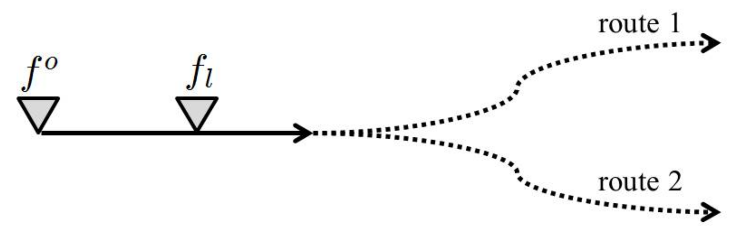
Normally, problem (15) is cheaper to solve than its counterpart (5), because in most practical cases $\left|\mathcal{O}\right||\tilde{\mathcal{L}}|<|\mathcal{R}|$, but its solution provides less information. Note that while recovering coefficients ${\beta }_l^o$ from known values ${\alpha }_{r^o}$ is straight forward, the reverse is not always possible, as shown by the trivial example presented in Figure 1. Here, $f^o=f_l$ and, thus, ${\beta }_l^o=1$, yet there is no information about how the flow is split between routes 1 and 2.

The complexity of the described problems depends on the choice of the least squares solver. According to [29], for a matrix with m rows and n columns with $m\ll n$, it ranges between $O\left(m{n}^2\right)$ and $O\left(n^3\right)$.

3.2. Accounting for Traffic Dynamics

Now, we consider the setup where flows $f^o\left(t\right)$, $o\in \mathcal{O}$, and $f_l\left(t\right)$, $l\in \tilde{\mathcal{L}}$, are measured continuously and speed information, $v_l\left(t\right)$, $l\in \mathcal{L}$, is available. (In reality, these measurement data are updated in discrete time intervals, e.g., every 30 s). Our goal is to find split coefficients ${\alpha }_{r^o}\left(t\right)$.

Suppose, at time step $t^{*}$, we obtain flow values $f_l\left(t^{*}\right)$ from all links with detection, $\tilde{\mathcal{L}}$. Knowing $v_l(·)$ (and thus, travel times, $\left|l\right|/v_l\left(t\right)$) on all links $\mathcal{L}$ for all time steps $t\le t^{*}$, we can compute for a given link $l\in \tilde{\mathcal{L}}$ and given route $r^o\in {\mathcal{R}}_l$, $o\in \mathcal{O}$, time $t_{l,r^o}^0$ when a vehicle using route $r^o$ had to leave origin o in order to reach link l at time $t^{*}$. Define the following:

$$\Delta =t^{*}-\underset{\begin{array}{c}l\in \tilde{\mathcal{L}};\\ r^o\in {\mathcal{R}}_l,o\in \mathcal{O}\end{array}}{min}{t}_{l,r^o}^0,$$

(16)

and denote the following.

$$t^0=t^{*}-\Delta .$$

(17)

Assuming the FIFO (First-In-First-Out—no overtaking) rule, any vehicle that left its origin before $t^0$ has already reached its destination, or at least left behind all the detectors on its route, by time $t^{*}$. Or, in other words, only those vehicles, leaving their destinations in the time interval $[t^0,t^{*})$ can contribute to the measured flows $f_l\left(t^{*}\right)$, $l\in \tilde{\mathcal{L}}$.

The analog of system (4a) in the time-dependent case can be represented as follows:

$$\left[\begin{array}{ccccc}{\Phi }_{|\tilde{\mathcal{L}}|\times \Delta |{\mathcal{R}}^1|}^1\left(t\right)& \cdots & {\Phi }_{|\tilde{\mathcal{L}}|\times \Delta |{\mathcal{R}}^o|}^o\left(t\right)& \cdots & {\Phi }_{|\tilde{\mathcal{L}}|\times \Delta |{\mathcal{R}}^{\left|\mathcal{O}\right|}|}^{\left|\mathcal{O}\right|}\left(t\right)\end{array}\right]\left[\begin{array}{c}{\mathit{\alpha }}_{\Delta |{\mathcal{R}}^1|\times 1}^1\left(t\right)\\ ⋮\\ {\mathit{\alpha }}_{\Delta |{\mathcal{R}}^o|\times 1}^o\left(t\right)\\ ⋮\\ {\mathit{\alpha }}_{\Delta |{\mathcal{R}}^{\left|\mathcal{O}\right|}|\times 1}^{\left|\mathcal{O}\right|}\left(t\right)\end{array}\right]=\left[\begin{array}{c}{f}_1\left(t^{*}\right)\\ ⋮\\ f_l\left(t^{*}\right)\\ ⋮\\ f_{\left|\mathcal{L}\right|}\left(t^{*}\right)\end{array}\right],$$

(18)

with relaxed constraints.

$$\sum _{r^o\in {\mathcal{R}}^o}{\alpha }_{r^o}\left(t\right)\le 1,t=t^0,\cdots ,t^{*};\forall o\in \mathcal{O}.$$

(19)

Here, we have the following:

$${\mathit{\alpha }}_{\Delta |{\mathcal{R}}^o|\times 1}^o\left(t\right)=\left[\begin{array}{c}{\mathit{\alpha }}_{|{\mathcal{R}}^o|\times 1}^o\left(t^0\right)\\ ⋮\\ {\mathit{\alpha }}_{|{\mathcal{R}}^o|\times 1}^o\left(t^{*}\right)\end{array}\right],$$

and the following is also the case.

$${\Phi }_{|\tilde{\mathcal{L}}|\times \Delta |{\mathcal{R}}^o|}^o\left(t\right)=\left\{{\varphi }_{l{r}^o}\left(t\right)\right\}\begin{array}{c}l=1,\cdots ,|\tilde{\mathcal{L}}|\hfill \\ t=t^0,\cdots ,t^{*};\hfill \\ r^o=1,\cdots ,\left|{\mathcal{R}}^o\right|\hfill \end{array},\mathrm{with} {\varphi }_{l{r}^o}\left(t\right)=\left\{\begin{array}{cc}{f}^o\left(t\right),\hfill & \mathrm{if} r^o\in {\mathcal{R}}_l \mathrm{and} t=t_{l,r^o}^0,\hfill \\ 0,\hfill & \mathrm{otherwise}.\hfill \end{array}\right.$$

Simplifying the notation, we rewrite (18) as follows.

$$\mathbf{\Phi }\left(t\right)\mathit{\alpha }\left(t\right)=\mathit{f}\left(t^{*}\right).$$

(20)

Adding nonnegativity constraints, we have the following.

$${\alpha }_{r^o}\left(t\right)\ge 0,t=t^0,\dots ,t^{*};r^o\in {\mathcal{R}}^o,\forall o\in \mathcal{O},$$

(21)

We cast the constrained least squares problem.

$$\underset{\begin{array}{c}\alpha \left(t\right)\ge \mathbf{0}\\ {\sum }_{r^o\in {\mathcal{R}}^o}{\alpha }_{r^o}\left(t\right)\le 1\end{array}}{min}{\parallel \mathbf{\Phi }\left(t\right)\mathit{\alpha }\left(t\right)-\mathit{f}\left(t^{*}\right)\parallel }_2^2.$$

(22)

In the situation of underdetermined system for the time-dependent case, we should impose sparsity constraints (as opposed to ${\ell }_2$ norm regularization) using either infinity norm replacement (8) or weighted ${\ell }_1$ norm penalty (9). The reason is that problem (22) is solved for one time instant $t^{*}$ only and, in general, for given time $t\in [t^0,t^{*})$ and given origin $o\in \mathcal{O}$, it allows us to recover only some coefficients ${\alpha }_{r^o}\left(t\right)$ but not all. Coefficients ${\alpha }_{r^o}\left(t\right)$ for routes not contributing to measurements at time $t^{*}$ will be nullified—see definition of ${\varphi }_{l{r}^o}\left(t\right)$ above. Hence, the relaxed constraints are obtained (19)—compare this with (2).

Constraints (19) may be modified as follows:

$$\sum _{r^o\in {\mathcal{R}}^o}{\alpha }_{r^o}\left(t\right)\le a^o\left(t\right),t=t^0,\dots ,t^{*};\forall o\in \mathcal{O},$$

(23)

where parameters $a^o\left(t\right)\in [0,1]$ are continuously updated using the recovered split coefficients ${\alpha }_{r^o}\left(t\right)$ as problem (22) is solved continuously, every time for new $t^{*}$. We start with $a^o\left(t\right)=1$ and then, after each iteration subtracts, the recovered coefficients ${\alpha }_{r^o}\left(t\right)$ from $a^o\left(t\right)$.

Once coefficients ${\alpha }_{r^o}\left(t\right)$, $t=t^0,\dots ,t^{*}$, are computed, for given link $l\in \tilde{\mathcal{L}}$ and time $t^{*}$, we derive the portion of measured flow $f_l\left(t^{*}\right)$ generated by the origin $o\in \mathcal{O}$, ${\beta }_l^o\left(t^{*}\right)$.

$${\beta }_l^o\left(t^{*}\right)=\frac{{\sum }_{\begin{array}{c}t=t^0,\dots ,t^{*};\\ r^o\in {\mathcal{R}}_l\end{array}}{\alpha }_{r^o}\left(t\right)f^o\left(t\right)}{f_l\left(t^{*}\right)}.$$

(24)

We note (without demonstrating) that it is possible to derive the dual problem analogous to (15) for the time-dependent case.

Finally, let us discuss how flow $f_{l^{+}}\left(t^{*}\right)$ at an arbitrary link $l^{+}\in \mathcal{L}$ can be computed if coefficients ${\alpha }_{r^o}\left(t\right)$, $t\le t^{*}$, are known. For each route $r\in {\mathcal{R}}_{l^{+}}$, using available speed data, we find the origin and time $t_{r,l^{+}}^0$, when vehicles had to leave that origin to arrive at link $l^{+}$ at time $t^{*}$. Thus, the following is the case.

$$f_{l^{+}}\left(t^{*}\right)=\sum _{\begin{array}{c}r\in {\mathcal{R}}_l;\\ r^o=r,o\in \mathcal{O}\end{array}}{\alpha }_{r^o}\left(t_{r,l^{+}}^0\right)f^o\left(t_{r,l^{+}}^0\right).$$

(25)

In the commonly used four-step demand model, route assignment is performed by an iterative process of flow balancing according to Wardrop’s principle of user equilibrium [30], where computational burden and accuracy heavily depend on the underlying dynamical traffic model. In contrast to that, we propose utilizing commercial speed data, for which its supply and affordability keep growing, for running a series of convex optimization problems resulting in (1) route assignment and (2) in flow estimates on all the link routes, which can be used for corridor performance computation and traffic control.

4. Selecting Plausible Routes

One obvious method of finding plausible routes between given origin and destination out of all possible ones, is to select several best routes for which their lengths are approximately equal. Introducing traffic dynamics modifies this problem: Utilizing user equilibrium principle [30], we replace lengths by travel times. Now, the question is how to pick plausible routes if travel times on them change throughout the day with traffic speed.

Suppose, we know all potential routes between the zones (i.e., for every O-D pair) and, hence, have the list of all links (belong to potential routes) that are used in our algorithm. We define the plausible route as the route that minimizes the travel time between an O-D pair. Since the travel time on a link depends on the traffic congestion in the road network, the plausible route changes based on the departure time from the origin and is time-dependent. Thus, we find the set of all plausible routes that minimizes travel-time throughout the day. Towards this end, we model the road-network as time-dependent weighted graph, where travel-cost of each link is a piecewise linear function of time, and the time-dependent fastest path for every O-D pair is computed.

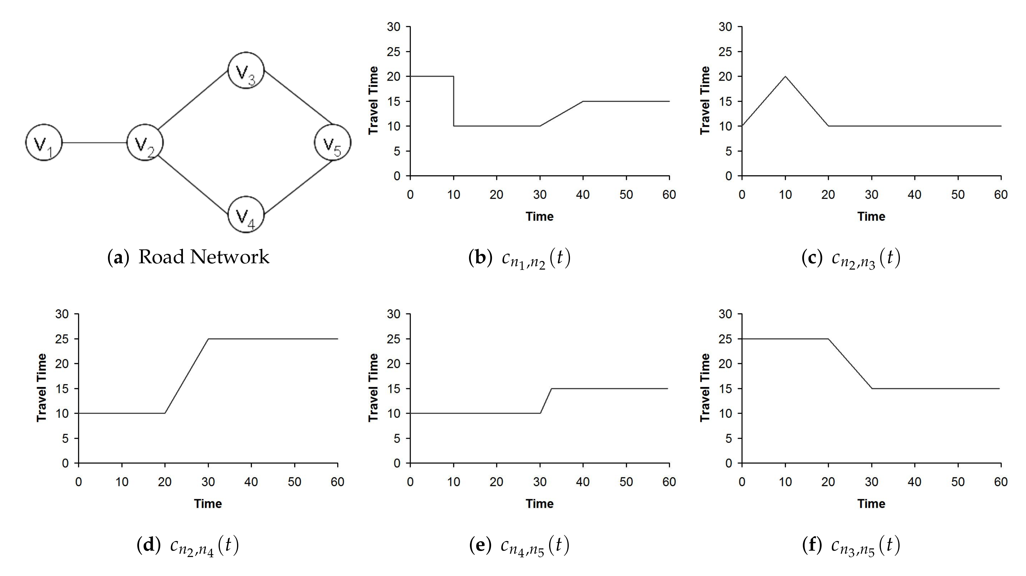
Time-dependent Graph: A Time-dependent Graph is defined as $G(\mathcal{N},\mathcal{L},T)$ where $\mathcal{N}=\left\{n_i\right\}$ is a set of nodes and $\mathcal{L}\subseteq \mathcal{N}\times \mathcal{N}$ is a set of links representing the network links each connecting two nodes. For every link $l(n_i,n_j)\in \mathcal{L}$ and $n_i\ne n_j$, there is a cost function $c_{n_i,n_j}\left(t\right)$, where t is the time variable in time domain T. The link cost function $c_{n_i,n_j}\left(t\right)$ specifies the travel-time from $n_i$ to $n_j$ starting at time t. In this paper, we assume that $G(\mathcal{N},\mathcal{L},T)$ satisfies the FIFO (First-In-First-Out) property. Figure 2 illustrates an example of time-dependent weighted graph, where link travel-times are function of time.

The travel-cost of any given path in $G(\mathcal{N},\mathcal{L},T)$ is time-dependent and defined as follows.

Time-dependent Travel Cost: Let $\{o=n_1,n_2,\dots ,n_k=d\}$ denote a path, which contains a sequence of nodes where $l(n_i,n_{i+1})\in \mathcal{L}$ and $i=1,\dots ,k-1$. Given a $G(\mathcal{N},\mathcal{L},T)$, a path $(o⇝d)$ from origin o to destination d and a departure-time at the origin $t_o$, the time-dependent travel cost $TT(o⇝d,t_o)$ is the time it takes to travel the path. Since the travel time of an link varies depending on the arrival time to that link, the travel time of a path is computed as follows.

$$TT(o⇝d,t_o)=\sum _{i=1}^{k-1}{c}_{n_i,n_{i+1}}\left(t_i\right), \mathrm{where} t_1=t_o, t_{i+1}=t_i+c_{(n_i,n_{i+1})}\left(t_i\right),i=1,\dots ,k.$$

We find a set of plausible routes by computing time-dependent fastest path for each O-D pair. Given a $G(\mathcal{N},\mathcal{L},T)$, o, d, and $t_o$, the time-dependent fastest path $TDFP(o,d,t_o)$ is a path with the minimum travel-time among all paths from o to d for starting time $t_o$. Time-dependent fastest problem in FIFO networks is polynomially solvable [31,32] by generalization of Dijkstra’s algorithm, where, analogous to shortest path distances, the arrival time to the nodes is used as the labels that form the basis of the greedy algorithm.

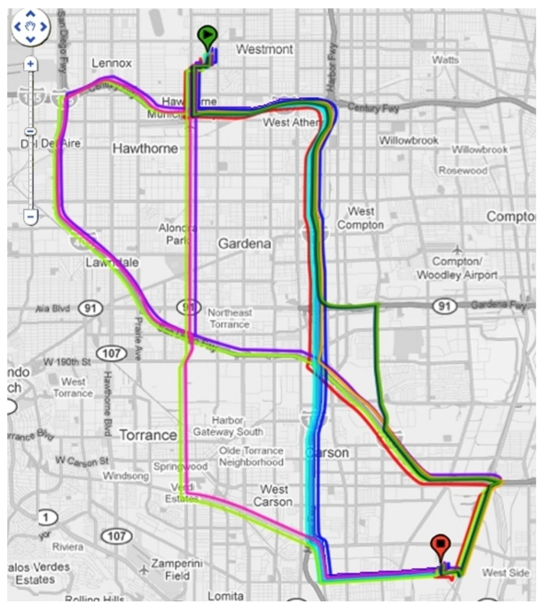
To illustrate this, consider Figure 3, which shows the set of fastest routes (i.e., plausible routes) for a hypothetical road network. The fastest routes are color coded for different departure times for the same origin and destination pair (each color represents the fastest route for a specific departure time). We computed time-dependent fastest paths for 48 consecutive departure-times between 7:00 a.m. and 7:00 p.m., spaced 15 min apart. As shown, there are a total of nine distinct plausible routes in this road networkm and they change during the course of the day.

5. Conclusions

We presented an algorithm for estimating how vehicle flows are split between routes in a given traffic network. The proposed method builds upon the compressed sensing technology, heavily used in image and signal processing, and uses state-of-the art techniques of introducing sparsity constraints to a convex optimization problem that already has a built-in ${\ell }_1$ norm constraint. The advantage of the proposed methodology is that it does not rely on simulation that is prone to calibration errors but only on measured data.

We showed the differences between the problem of computing coefficients that split origin flows between routes and the problem of computing the portions of measured flows contributed by given origins. The latter problem is more computationally friendly, but it is less informative. We also discussed how vehicle flows can be estimated at links with no detection. This is important because it allows us to compute the following performance measures on the network scale as well as for individual sub-route inside the road network: vehicle miles (Kilometers) traveled, emissions with assumption on the portion of hybrids, electrical vehicles, trucks in the mixed traffic flow, vehicle hours traveled, delay and productivity loss.

In the latter case, we would be able to break up the values of these performance measures by origin.

Finally, the method for selecting plausible routes between origins and destinations taking into account the changing traffic state was suggested.

References

- Van Zyulen, H.; Willumsen, L. The most likely trip matrix estimated from traffic counts. Transp. Res. Part B 1980, 14, 281–293. [Google Scholar] [CrossRef]
- Cascetta, E. Estimation of trip matrices from traffic counts and survey data: A generalized least squares estimator. Transp. Res. Part B 1984, 18, 289–299. [Google Scholar] [CrossRef]
- Bell, M. The real time estimation of origin-destination flows in the presence of platoon dispersion. Transp. Res. Part B 1991, 25, 115–125. [Google Scholar] [CrossRef]
- Krishnakumaria, P.; van Lint, H.; Djukic, T.; Cats, O. A data driven method for OD matrix estimation. Transp. Res. Part C 2020, 113, 38–56. [Google Scholar] [CrossRef] [Green Version]
- Willumsen, L. Estimation of an O-D Matrix from Traffic Counts—A Review; Working Paper 99; Institute of Transport Studies, University of Leeds: Leeds, UK, 1978. [Google Scholar]
- Evans, S. A relationship between the gravity model for trip distribution and the transportation problem in linear programming. Transp. Res. 1973, 7, 38–56. [Google Scholar] [CrossRef]
- Wardrop, J.G. Some Theoretical Aspects of Road Traffic Research. Proc. Inst. Civ. Eng. Part II 1952, 1, 325–378. [Google Scholar] [CrossRef]
- Chiu, Y.C.; Bottom, J.; Mahut, M.; Paz, A.; Balakrishna, R.; Waller, T.; Hicks, J. Dynamic Traffic Assignment. A Primer; Technical Report Circular E-153; Transportation Research Board: Washington, DC, USA, 2011. [Google Scholar]
- Kitamura, R.; Chen, C.; Pendyala, R.; Narayanan, R. Micro-simulation of daily activity-travel patterns for travel demand forecasting. Transportation 2000, 27, 25–51. [Google Scholar] [CrossRef]
- Bhat, C.; Zhao, H. The spatial analysis of activity stop generation. Transp. Res. Part B 2002, 36, 557–575. [Google Scholar] [CrossRef] [Green Version]
- Arrentze, T.; Timmermans, H. A need-based model of multi-day, multi-person activity generation. Transp. Res. Part B 2009, 43, 253–265. [Google Scholar] [CrossRef]
- Cantelmo, G.; Viti, F.; Cipriani, E.; Nigro, M. A Two-Steps Dynamic Demand Estimation Approach Sequentially Adjusting Generations and Distributions. In Proceedings of the Intelligent Transportation Systems Conference (ITSC), Gran Canaria, Spain, 15–18 September 2015; pp. 1477–1482. [Google Scholar]
- Scheffer, A.; Cantelmo, G.; Viti, F. Generating macroscopic, purpose-dependent trips through Monte Carlo sampling techniques. Transp. Res. Procedia 2017, 27, 585–592. [Google Scholar] [CrossRef]
- Cremer, M.; Keller, H. A new class of dynamic methods for the identification of origin-destination flows. Transp. Res. Part B 1987, 21, 117–132. [Google Scholar] [CrossRef]
- Yang, H.; Sasaki, T.; Iida, Y.; Asakura, Y. Estimation of origin-destination matrices from link traffic counts on congested networks. Transp. Res. Part B 1992, 26, 417–434. [Google Scholar] [CrossRef]
- Ashok, K.; Ben-Akiva, M. Alternative approaches for real-time estimation and prediction of time-dependent origin-destination flows. Transp. Sci. 2000, 32, 21–36. [Google Scholar] [CrossRef] [Green Version]
- Zhou, X.; Mahmassani, H. A structural state space model for real-time traffic origin-destination demand estimation and prediction in a day-to-day learning framework. Transp. Res. Part B 2007, 41, 823–840. [Google Scholar] [CrossRef]
- Castillo, E.; Rivas, A.; Jimenez, P.; Menendez, J. Observability in traffic networks. Plate scanning added by counting information. Transportation 2012, 39, 1301–1333. [Google Scholar] [CrossRef]
- Cascetta, E. Transportation Systems Engineering: Theory and Methods; Springer Science & Business Media: Berlin/Heidelberg, Germany, 2013; Volume 47. [Google Scholar]
- Cantelmo, G.; Cipriani, E.; Gemma, A.; Nigro, M. An adaptive bi-level gradient procedure for the estimation of dynamic traffic demand. IEEE Trans. Intell. Transp. Syst. 2014, 15, 1348–1361. [Google Scholar] [CrossRef]
- Cipriani, E.; Nigro, M.; Fusco, G.; Colombaroni, C. Effectiveness of link and path information on simultaneous adjustment of dynamic O-D demand matrix. Eur. Transp. Res. Rev. 2014, 6, 139–148. [Google Scholar] [CrossRef] [Green Version]
- Antoniou, C.; Barcelo, J.; Breenc, M.; Bullejosb, M.; Casos, J.; Cipriani, E.; Ciuffo, B.; Djukic, T.; Hoogendoorn, S.; Marzano, V.; et al. Towards a generic benchmarking platform for origin–destination flows estimation/updating algorithms: Design, demonstration and validation. Transp. Res. Part C 2016, 66, 79–98. [Google Scholar] [CrossRef]
- Bera, S.; Krishna Rao, K.V. Estimation of Origin-Destination Matrix from Traffic Counts: The State of the Art. Eur. Transp. 2011, 49, 3–23. [Google Scholar]
- Meyer, M.; Miller, E. Urban Transportation Planning, 2nd ed.; McGraw-Hill: New York, NY, USA, 2000. [Google Scholar]
- Donoho, D.L. Compressed Sensing. IEEE Trans. Inf. Theory 2006, 52, 1289–1306. [Google Scholar] [CrossRef]
- Tikhonov, A.N. Solution of Incorrectly Formulated Problems and the Regularization Method. Dokl. Akad. Nauk SSSR 1963, 151, 501–504. [Google Scholar]
- Pilanci, M.; El Ghaoui, L.; Chandrasekaran, V. Recovery of Sparse Probability Measures via Convex Programming. In Proceedings of the Advances in Neural Information Processing Systems (NIPS), Lake Tahoe, NV, USA, 3–6 December 2012. [Google Scholar]
- Candes, E.J.; Wakin, M.B.; Boyd, S. Enhancing Sparsity by Reweighted l1 Minimization. J. Fourier Anal. Appl. 2008, 14, 877–905. [Google Scholar] [CrossRef]
- Lee, D. Numerically Efficient Methods for Solving Least Squares Problems; University of Chicago: Chicago, IL, USA, 2012. [Google Scholar]
- Wardrop, J.G.; Whitehead, J.I. Correspondence. Some Theoretical Aspects of Road Traffic Research. ICE Proc. Eng. Div. 1952, 1, 767–768. [Google Scholar] [CrossRef]
- Dreyfus, S.E. An Appraisal of Some Shortest-Path Algorithms. Oper. Res. 1969, 17, 395–412. [Google Scholar] [CrossRef]
- Halpern, J. Shortest Route with Time-dependent Length of Edges and Limited Delay Possibilities in Nodes. Oper. Res. 1977, 21, 117–124. [Google Scholar] [CrossRef]
Figure 1.
Example: , while and are unknown.
Figure 2.
A Time-dependent Graph .
Figure 3.
Set of plausible routes for a pair of origin and destination in a hypothetical road network.