A Note on Pareto-Type Distributions Parameterized by Its Mean and Precision Parameters

Abstract

Pareto-type distributions are well-known distributions used to fit heavy-tailed data. However, the standard parameterizations used for Pareto-type distributions are poorly suited to modeling. On this note, we suggest new parameterizations that are better suited to the purpose. In addition, we propose many regression models where the response variable is Pareto-type distributed using new parameterizations that are indexed by mean and precision parameters. The main motivation for these new parametrizations is the useful interpretation of the regression coefficients in terms of the mean and precision, as is usual in the context of regression models. The parameter estimation of these new models is performed, based on the maximum likelihood paradigm. Some numerical illustrations of the estimators are presented with a discussion of the obtained results. Finally, we illustrate the practicality of the new models by means of two applications to real data sets.

1. Introduction

The Pareto distribution was originally applied by Pareto [1] to model the unequal distribution of wealth. Despite being proposed a long time ago, there are still many current works that use this distribution. See, for instance, the works of Wang and Li [2], Shrahili et al. [3] and Sharpe and Juárez [4], to name a few. The random variable Y has the Pareto distribution if its cumulative distribution function (CDF) for $y\ge \beta$ is given by

$$F(y;\alpha ,\beta )=1-{\left(\frac{\beta }{y}\right)}^{\alpha },$$

(1)

where $\beta >0$ is a scale parameter and $\alpha >0$ is a shape parameter. The parameter $\beta$ is only a scale factor, which is known as the tail index. When this distribution is used to model the distribution of wealth, the parameter $\alpha$ a is called the Pareto index. Here, this distribution is called Pareto Type I distribution (Pareto [5]).

The Lomax distribution (Lomax [6]), also called the Pareto Type II distribution, is a Pareto Type I distribution shifted so that its support begins at zero. Its CDF is of the form

$$F(y;\alpha ,\beta )=1-{\left(1+\frac{y}{\beta }\right)}^{-\alpha },y>0.$$

(2)

There is a relation between the Pareto Type II distribution and the generalized Pareto distribution (GPD), which is much used in the study of extreme values and peaks over thresholds. The CDF of the GPD is given by (Pickands [7])

$$\begin{array}{c}\hfill F(y;\sigma ,\xi )=1-{\left(1+\alpha \frac{y}{\beta }\right)}^{-1/\alpha }.\end{array}$$

Regression models are typically constructed to model the mean of a distribution. Despite the nice properties of Pareto-type distributions, none of their parameters correspond to the expectation, which complicates the interpretation of regression models specified using these distributions. In this context, we proposed a new parameterization of these distributions that is indexed by mean and precision parameters. Parameterizations of statistical models are not unique. In general, we use a particular parameterization for interpretation of the parameters and/or for computational convenience. The current manuscript falls into the first category (interpretation of the parameters). The main advantage of our new parametrization is the straightforward interpretation of the regression coefficients in terms of the expectation of the positive real line response variable, as is usual in the context of generalized linear models.

The paper is organized as follows. In Section 2, we present new parameterizations of the Pareto-type distributions indexed by mean and precision parameters. Section 3 introduces the Pareto-type regression models with varying mean and precision. Furthermore, numerical results from Monte Carlo simulation experiments are presented and discussed. In Section 4, we provide the applications to two real data sets. Concluding remarks and possible points for future research are given in the Section 5.

2. Pareto-Type Distributions with Alternative Parameterizations

In this Section, we provide four reparameterizations for Pareto-type distributions indexed by mean and dispersion parameters.

2.1. Pareto Distribution

The probability density function (PDF) related to the Pareto model with PDF indicated in Equation (1) is given by

$$f(y;\alpha ,\beta )=\alpha {\beta }^{\alpha }{y}^{-(\alpha +1)},y\ge \beta .$$

(3)

The mean and variance of the distribution are given by

$$\mathrm{E}\left(Y\right)=\frac{\alpha \beta }{\alpha -1},\alpha >1\mathrm{and}\mathrm{Var}\left(Y\right)=\frac{\alpha {\beta }^2}{(\alpha -2){(\alpha -1)}^2},\alpha >2,$$

(4)

respectively. In practice, $\alpha$ is frequently assumed to be larger than 2, so that the distribution has a finite variance.

A new parameterization of the Pareto distribution given by $\mu =\alpha \beta /(\alpha -1)>0$ and $\varphi =\alpha (\alpha -2)>0$, i.e., $\alpha =1+\sqrt{1+\varphi }>2$ and $\beta =\left(\mu \sqrt{1+\varphi }\right)/(1+\sqrt{1+\varphi })>0$. With this new parameterization, it follows from (4) that

$$\mathrm{E}\left(Y\right)=\mu \mathrm{and}\mathrm{Var}\left(Y\right)=\frac{{\mu }^2}{\varphi }.$$

Henceforth, we consider the notation $Y\sim \mathrm{RPa}(\mu ,\varphi )$ to specify that Y is a random variable following a reparameterized Pareto model, with mean $\mu >0$ and precision parameter $\varphi >0$. We highlight that, up to this moment, this parameterization has not been proposed in the literature.

Using the proposed parameterization, the RPa density in (3) can be written as

$$f(y;\mu ,\varphi )=[1+\sqrt{1+\varphi }]{\left(\frac{\mu \sqrt{1+\varphi }}{1+\sqrt{1+\varphi }}\right)}^{1+\sqrt{1+\varphi }}{y}^{-(1+\sqrt{1+\varphi }+1)},y\ge \frac{\mu \sqrt{1+\varphi }}{1+\sqrt{1+\varphi }}.$$

(5)

2.2. Power Function Distribution

The power function model is a two-parameter distribution, which is the distribution of the reciprocal of a variable distributed according to the Pareto distribution, i.e., if X has a Pareto distribution with parameters $\alpha$ and $\beta$, then $Y=X^{-1}$ has a power function distribution with parameters $\alpha >0$ (shape parameter) and $\beta >0$ (scale parameter).

We begin with the PDF of the power function distribution given by

$$f(y;\alpha ,\beta )=\alpha {\beta }^{-\alpha }{x}^{\alpha -1},0<x<\beta .$$

(6)

The mean and variance of Y are

$$\mathrm{E}\left(Y\right)=\frac{\alpha \beta }{\alpha +1}\mathrm{and}\mathrm{Var}\left(Y\right)=\frac{\alpha {\beta }^2}{(\alpha +2){(\alpha +1)}^2}.$$

(7)

A new parameterization of the power function distribution is given by $\mu =\alpha \beta /(\alpha +1)>0$ and $\varphi =\alpha (\alpha +2)$, i.e., $\alpha =\sqrt{1+\varphi }-1$ and $\beta =\mu \sqrt{1+\varphi }/(\sqrt{1+\varphi }-1)$. With this new parameterization, it follows from (7) that

$$\mathrm{E}\left(Y\right)=\mu \mathrm{and}\mathrm{Var}\left(Y\right)=\frac{{\mu }^2}{\varphi }.$$

Hereafter, we consider the notation $Y\sim \mathrm{RPo}(\mu ,\varphi )$ to specify that Y is a random variable following a reparameterized power function distribution, with mean $\mu$ and precision parameter $\varphi >0$. We remark that this parameterization has not been proposed in the statistical literature.

Using this alternative parameterization, the PDF for the RPO distribution in (6) can be written as

$$f(y;\mu ,\varphi )=[\sqrt{1+\varphi }-1]{[\mu \sqrt{1+\varphi }/(\sqrt{1+\varphi }-1)]}^{1-\sqrt{1+\varphi }}{x}^{\sqrt{1+\varphi }-2},0<y<\mu \sqrt{1+\varphi }/(\sqrt{1+\varphi }-1).$$

(8)

2.3. Lomax Distribution

The PDF associated to a dislocated Pareto in (2) is given by

$$f(y;\alpha ,\beta )=\frac{\alpha {\beta }^{\alpha }}{{(y+\beta )}^{\alpha +1}},y\ge 0.$$

(9)

The mean and the variance for (9) are given by

$$\mathrm{E}\left(Y\right)=\frac{\beta }{\alpha -1},\alpha >1\mathrm{and}\mathrm{Var}\left(Y\right)=\frac{\alpha {\beta }^2}{(\alpha -2){(\alpha -1)}^2},\alpha >2.$$

(10)

We considered an alternative parameterization of the Lomax distribution in terms of the mean and precision parameters. Define $\mu =\beta /(\alpha -1)>0$ and $\varphi =\alpha -2>0$, i.e., $\alpha =\varphi +2>2$ and $\beta =\mu (\varphi +1)>0$. With this alternative parameterization, it follows from (10) that

$$\mathrm{E}\left(Y\right)=\mu \mathrm{and}\mathrm{Var}\left(Y\right)=\frac{{\mu }^2(\varphi +2)}{\varphi }={\mu }^2\omega {\left(\varphi \right)}^2,$$

where $\omega \left(\varphi \right)=\sqrt{\frac{\varphi +2}{\varphi }}$ represents the coefficient of variation of Y, which depends only on $\varphi >0$. Moreover, $\varphi$ represents a precision parameter because, for a fixed $\mu$, and an increasing $\varphi$, the corresponding variance decreases. From now on, we use the notation $Y\sim \mathrm{RLo}(\mu ,\varphi )$ to indicate that Y has a reparameterized Lomax distribution with mean $\mu >0$ and precision parameter $\varphi >0$. We highlight that this parameterization has not been proposed in the statistical literature. Using the proposed parameterization, we can write the RLo PDF as

$$f(y;\mu ,\varphi )=\frac{[\varphi +2]{\left[\mu (\varphi +1)\right]}^{\varphi +2}}{{[y+\mu (\varphi +1)]}^{\varphi +3}},y\ge 0.$$

(11)

2.4. Generalized Pareto Distribution

The GPD (Pickands [7]) is a two-parameter family of distributions, with PDF given by

$$f(y;\alpha ,\beta )=\frac{1}{\beta }{\left(1+\frac{\alpha y}{\beta }\right)}^{-\left(\frac{1}{\alpha }+1\right)},$$

(12)

where $\beta >0$ and $\alpha$ are the scale and shape parameters, respectively. For $\alpha >0$ the range of y is $0<y<\beta /\alpha$ and for $\alpha <0$ the range is $y>0$. One of the interesting features of this distribution is its simple mathematical form.

The mean and the variance associated with (12) are given by

$$\mathrm{E}\left(Y\right)=\frac{\beta }{1-\alpha },\alpha <1\mathrm{and}\mathrm{Var}\left(Y\right)=\frac{{\beta }^2}{{(1-\alpha )}^2(1-2\alpha )},\alpha <1/2,$$

(13)

respectively.

A new insight into the GPD can be obtained by performing a reparameterization on the random variable X, whose PDF is given in (12). Consider the parameterization $\mu =\beta /(1-\alpha )>0$ and $\varphi =1-2\alpha >0$, i.e., $\beta =\mu (1+\varphi )/2>0$ and $\alpha =(1-\varphi )/2>2$. With this alternative parameterization, it follows from (13) that

$$\mathrm{E}\left(Y\right)=\mu \mathrm{and}\mathrm{Var}\left(Y\right)=\frac{{\mu }^2}{\varphi }.$$

Hereafter, we use $Y\sim \mathrm{RGPD}(\mu ,\varphi )$ to say that Y follows a reparameterized GPD distribution with mean $\mu >0$ and precision $\varphi >0$. We also note that this parameterization is already known in the statistical literature (see, for instance, Bourguignon and do Nascimento [8]). Thus, the RGPD PDF in equation (12) can be written as

$$f(y;\mu ,\varphi )=\frac{2}{\mu (1+\varphi )}{\left[1+\frac{(1-\varphi )y}{\mu (1+\varphi )}\right]}^{-\frac{3-\varphi }{1-\varphi }}.$$

(14)

2.5. Other Models Parameterized in Terms of the Mean and Precision Parameters

For the RPa and RLo models, we considered the restriction $\alpha >2$ and for the RGPD model we take into account the restriction $\alpha <1/2$, in order to guarantee the existence of the mean and variance terms. In principle, this can be a disadvantage because the class of models that we are considering is smaller than the original proposals. In return, we obtain models where, under some conditions, the coefficients can be interpreted in a very useful way, as we will see in the Section 3.

In the literature, there are many models with positive support parameterized in terms of the mean, and with a quadratic form to the variance, i.e, the mean and variance of the model are given by $\mu$ and ${\mu }^2{\left[\omega \left(\varphi \right)\right]}^2$, respectively, where $\mu ,\varphi >0$ and $\omega (·)$ is a positive function. To name a few examples, we referred to the reparametrized gamma and Weibull models, both available with the GA and WEI3 functions in the gamlss.dist [9] package of the software R [10]; the reparameterized Birnbaum-Saunders model [11]; the reparameterized slash half-normal distribution [12]; among others. The recommendation is to fit part of such models and, based on model selection criteria such as the Akaike [13] (AIC) and Schwartz [14] (BIC) criteria, choose a model and validate it based on some kind of residuals. For instance, we suggest the quantile residuals (QR) discussed in Dunn and Smyth [15].

3. Modelling and Inference

The main advantage of the reparameterization of models in terms of the mean is the possible interpretation of the coefficients when a regression structure is incorporated into the mean. For this, let $Y_1,\dots ,Y_n$ be n independent random variables, where each $Y_i$, $i=1,\dots ,n$, follows the PDF given in Equation (5), (8), (11) or (14), depending on whether we are interest in the use of the RPa, RPo, RLo or RGPD model, with mean ${\mu }_i$ and precision parameter ${\varphi }_i$. In order to introduce a regression structure in the Pareto-type models, we assume that

$$g_1\left({\mu }_i\right)={\eta }_{1i}={\mathbf{x}}_i^{\top }\beta \mathrm{and}{g}_2\left({\varphi }_i\right)={\eta }_{2i}={\mathbf{z}}_i^{\top }\nu ,$$

(15)

where $\beta ={({\beta }_1,\dots ,{\beta }_p)}^{\top }$ and $\nu ={({\nu }_1,\dots ,{\nu }_q)}^{\top }$ are vectors of unknown regression coefficients, which we assumed to be functionally independent, $\beta \in {\mathbb{R}}^p$ and $\nu \in {\mathbb{R}}^q$, with $p+q<n$, ${\eta }_{1i}$ and ${\eta }_{2i}$ are the linear predictors, and ${\mathbf{x}}_i={(x_{i1},\dots ,x_{ip})}^{\top }$ and ${\mathbf{z}}_i={(z_{i1},\dots ,z_{iq})}^{\top }$ are p and q known regressors, respectively, for $i=1,\dots ,n$. Additionally, we assume that the rank of $\mathbf{X}={({\mathbf{x}}_1,\dots ,{\mathbf{x}}_n)}^{\top }$ and $\mathbf{Z}={({\mathbf{z}}_1,\dots ,{\mathbf{z}}_n)}^{\top }$ are p and q, respectively. The link functions $g_1:\mathbb{R}\to {\mathbb{R}}^{+}$ and $g_2:\mathbb{R}\to {\mathbb{R}}^{+}$ in (15) must be strictly monotone, positive and at least twice differentiable, such that ${\mu }_i=g_1^{-1}\left({\mathbf{x}}_i^{\top }\beta \right)$ and ${\varphi }_i=g_2^{-1}\left({\mathbf{z}}_i^{\top }\nu \right)$, with $g_1^{-1}(·)$ and $g_2^{-1}(·)$ being the inverse functions of $g_1(·)$ and $g_2(·)$, respectively.

For the case where $g_1\left(u\right)=exp\left(u\right)$, the interpretations about the components of $\beta$ are as following:

• $exp\left({\beta }_0\right)$ represents the mean of the response variable when all the covariates are equal to 0. Of course, this interpretation is valid as long as it makes sense.
• $exp\left({\beta }_j\right)$, $j=1,\dots ,p$ represents the increment (in percentage terms) when the j-th covariates increased in 1 unit and the others are fixed.

On the other hand, the log-likelihood function is given by

$$\begin{array}{c}\hfill \ell (\beta ,\nu )=\sum _{i=1}^n\ell ({\mu }_i,{\varphi }_i),\end{array}$$

where $\ell ({\mu }_i,{\varphi }_i)=logf(y_i;{\mu }_i,{\varphi }_i)$, with $f(y_i;{\mu }_i,{\mu }_i)$ the PDF given in Equation (5), (8), (11) or (14), depending on the reparameterized model to be used.

The maximum likelihood (ML) estimators of $\beta$ and $\nu$, say $\widehat{\beta }$ and $\widehat{\nu }$, respectively, can be obtained by solving simultaneously the nonlinear system of equations $\partial \ell (\beta ,\nu )/\partial \beta =0$ and $\partial \ell (\beta ,\nu )/\partial \nu =0$. However, no closed-form expressions for the ML estimates are obtained, except in the Pareto and Lomax models in the case where $x_i=z_i=1$, for $i=1,\dots ,n$, i.e., for the instance where only the intercept term is included in both set of covariates. Therefore, we must use an iterative method for nonlinear optimization.

A Simulation Study

Here, we present a simulation study. For this, we consider the RLo model and the same covariate to model the parameters $\mu$ and $\varphi$. The covariates were drawn from the uniform distribution. We considered two combinations of parameters: scenario 1, ${\beta }_0=1.5$, ${\beta }_1=0.8$, ${\nu }_0=-1.2$ and ${\nu }_1=0.7$ and; scenario 2, ${\beta }_0=-2.1$, ${\beta }_1=1.3$, ${\nu }_0=0.8$ and ${\nu }_1=1.2$. We also considered three sample sizes: 50, 100, and 200. For each combination of parameters, we drew 1000 replicates of the respective sample size and compute the maximum likelihood estimators and their respective estimated standard errors.

Table 1. Estimated bias, standard errors and coverage probabilities for the estimators in the reparametrized Lomax model.

		$\mathit{n}=50$			$\mathit{n}=100$			$\mathit{n}=200$
Scenario	Estimator	bias	se	cp	bias	se	cp	bias	se	cp
1	${\beta }_0$	−0.0604	0.4442	0.909	−0.0481	0.2941	0.941	−0.0254	0.2046	0.947
	${\beta }_1$	−0.0326	0.6318	0.929	−0.0125	0.4417	0.935	−0.0052	0.3351	0.941
	${\nu }_0$	0.0669	0.6213	0.968	0.0407	0.5665	0.961	0.0316	0.4049	0.955
	${\nu }_1$	0.0934	0.5640	0.960	0.0689	0.4717	0.958	0.0283	0.3449	0.953
2	${\beta }_0$	−0.0992	0.4245	0.909	−0.0616	0.2895	0.930	−0.0427	0.1885	0.949
	${\beta }_1$	0.0562	0.6192	0.920	0.0487	0.4412	0.932	0.0308	0.3064	0.946
	${\nu }_0$	0.0634	0.9408	0.938	0.0417	0.7089	0.941	0.0307	0.6292	0.945
	${\nu }_1$	0.0764	0.6649	0.936	0.0658	0.4683	0.943	0.0357	0.3787	0.946

summarizes the mean bias (bias), the mean of the estimated standard errors (se), and the respective 95% coverage probabilities (cp). Results suggest that the bias for all the cases is acceptable, and both the bias and the se terms are reduced when the sample size is increased. Additionally, the coverage probabilities are closer to the nominal value when n is increased. Those results suggest that the estimators for the RLo model are consistent.

4. Real-World Data Analysis

In this section, we present two applications of the proposed models using real data for illustrative purposes.

4.1. Lomax Regression Model

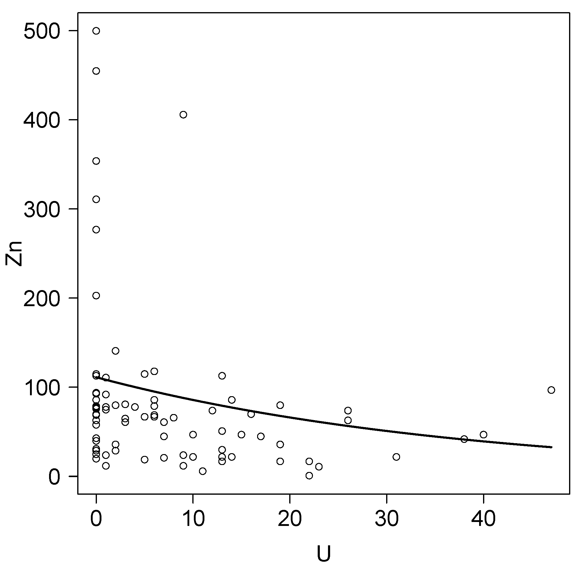
This data set was obtained from the Department of Mining of the University of Atacama, Chile, to study the concentration of some ores in the soil. The data set corresponds to 86 measurements of the concentration of the Zinc (Zn) and Uranium (U) ore respectively, both in parts per million (ppm). We consider a regression model to explain the quantity of Zn in terms of the quantity of U. For this, we considered that ${\mathtt{Zn}}_i\sim \mathrm{RLo}({\mu }_i,{\varphi }_i)$, where

$${\mu }_i=exp({\beta }_0+{\beta }_1\times {\mathtt{U}}_i)and{\varphi }_i=exp({\nu }_0+{\nu }_1\times {\mathtt{U}}_i),i=1,\dots ,86.$$

(16)

For comparative purposes, we also considered $y_i\sim \mathrm{RGa}({\mu }_i,{\varphi }_i)$, a reparametrized version of the gamma distribution such as $\mathrm{E}\left(Y_i\right)={\mu }_i$ and Var$\left(Y_i\right)={\mu }_i^2{\varphi }_i^2$, a very similar structure for the mean and variance as the RLo model, where ${\mu }_i$ and ${\varphi }_i$ are defined based on the regression structure given in (16).

Table 2. Estimated parameters in mineral data set.

	RGa		RLo
	Estimate	se	Estimate	se
${\beta }_0$	4.7518	0.1198	4.7114	0.1572
${\beta }_1$	−0.0288	0.0100	−0.0260	0.0108
${\nu }_0$	−0.1212	0.0915	1.2420	0.9530
${\nu }_1$	0.0041	0.0079	0.0187	0.0732
AIC	958.01		953.79
BIC	967.83		963.61

shows the results for these models. Note that the RLo model presents lower AIC and BIC criteria, suggesting the use of the RLo model instead of the RGa model for this particular problem. Additionally, as $exp\left({\widehat{\beta }}_1\right)=0.974$, the mean of Zn decrease in 2.6% (95% confidence interval 1.5–3.6%) for each ppm in which U is increased. Finally, Figure 1 shows the estimated mean for Zn for each value of U.

4.2. Pareto Regression Model

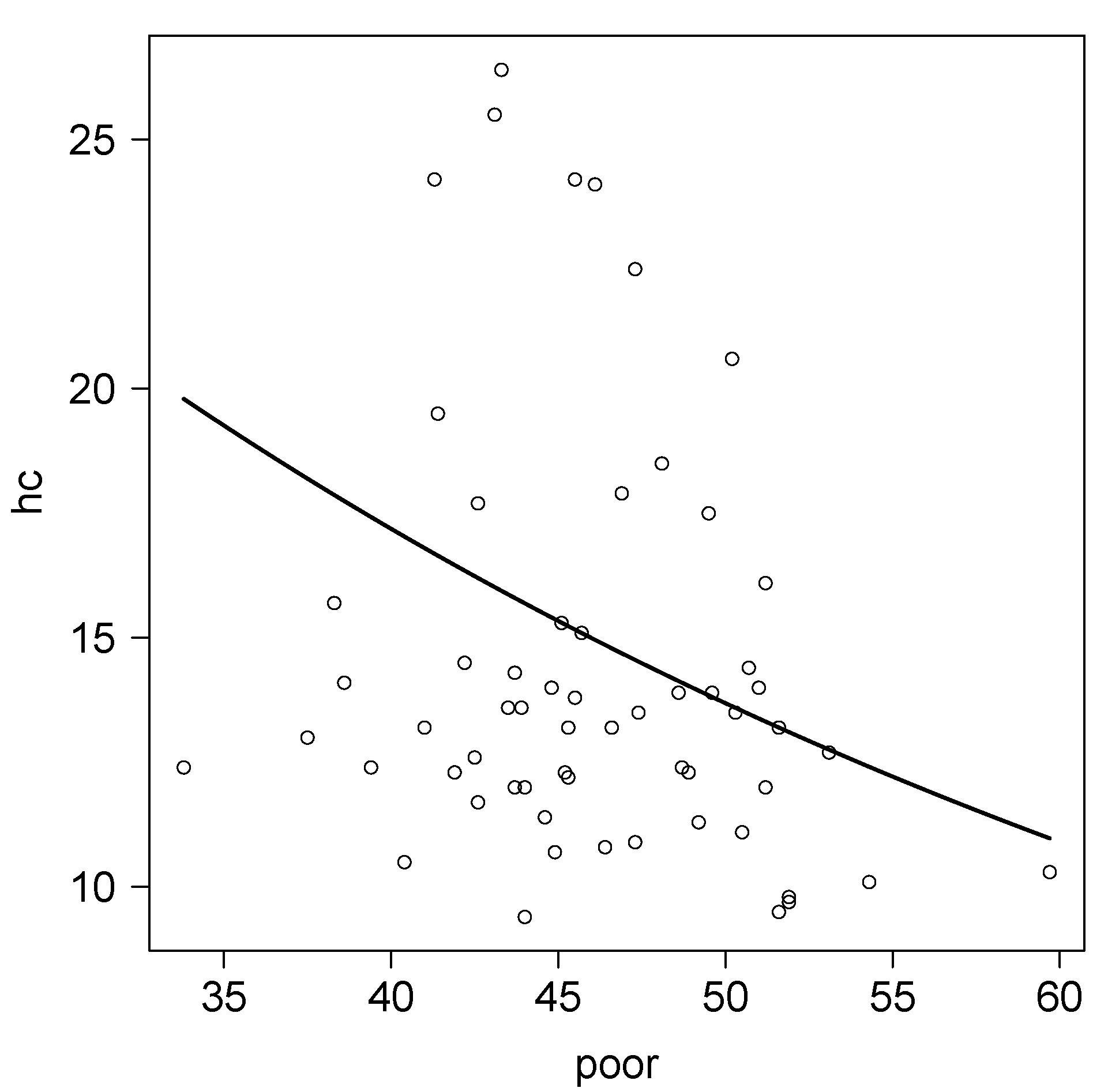
This data set was presented in Gunst and Mason (1980). The data set gives different measure of air pollution, and environmental, demographic and socioeconomic variables for 60 Standard Metropolitan Statistical Areas of the United States. We considered the percent of families with income under $3000 (poor) and the relative pollution potential of hydrocarbons (hc). We consider a regression model to explain hc in terms of poor, considering that ${\mathtt{hc}}_i\sim \mathrm{RPa}({\mu }_i,{\varphi }_i)$, where

$${\mu }_i=exp({\beta }_0+{\beta }_1\times {\mathtt{poor}}_i)and{\varphi }_i=exp({\nu }_0+{\nu }_1\times {\mathtt{poor}}_i),i=1,\dots ,60.$$

(17)

For comparative purposes, we also considered $y_i\sim \mathrm{RWe}({\mu }_i,{\varphi }_i)$, a reparameterized version of the Weibull distribution such as $\mathrm{E}\left(Y_i\right)={\mu }_i$ and Var$\left(Y_i\right)={\mu }_i^2\mathsf{\Gamma }(1/{\varphi }_i+1)/{\mathsf{\Gamma }}^2(1/{\varphi }_i+1)$, again a very similar structure for the mean and variance as the RPa model, where ${\mu }_i$ and ${\varphi }_i$ are defined based on the regression structure given in (17).

Table 3. Estimated parameters in metropolitan areas of USA data set.

	RWe		RPa
	Estimate	se	Estimate	se
${\beta }_0$	3.7712	0.3870	3.7549	0.8921
${\beta }_1$	−0.0239	0.0080	−0.0228	0.0175
${\nu }_0$	−0.9357	1.1873	−8.5153	1.3215
${\nu }_1$	0.0487	0.0255	0.1982	0.0132
AIC	345.11		326.47
BIC	353.48		334.84

shows the results for this case. Note that the RPa model presents lower AIC and BIC criteria, suggesting the use of the RPa model instead of the RWe model for this particular problem. Finally, Figure 2 shows the estimated mean for hc for each value of poor.

5. More Concluding Remarks and Discussion

In this work, we study new parameterizations for the Pareto-type distributions in terms of the mean and precision parameters. Furthermore, we have proposed regression models where the response variable is Pareto-type distributed using these new parameterizations. The models’ parameters are estimated by the maximum likelihood method. A Monte Carlo simulation study shows that the maximum likelihood estimators have a reasonable behavior. Finally, the usefulness of the proposed methodology is shown through two applications.

References

- Pareto, V. Cours d’economie Politique; F. Rouge: Lausanne, Switzerland, 1987; Volume II. [Google Scholar]
- Wang, X.; Li, X. Generalized Confidence Intervals for Zero-Inflated Pareto Distribution. Mathematics 2021, 9, 3272. [Google Scholar] [CrossRef]
- Shrahili, M.; Al-Omari, A.I.; Alotaibi, N. Acceptance Sampling Plans from Life Tests Based on Percentiles of New Weibull–Pareto Distribution with Application to Breaking Stress of Carbon Fibers Data. Processes 2021, 9, 2041. [Google Scholar] [CrossRef]
- Sharpe, J.; Juárez, M.A. Estimation of the Pareto and related distributions—A reference-intrinsic approach. Commun. Stat.-Theory Methods 2021. [Google Scholar] [CrossRef]
- Arnold, B.C. Pareto Distribution; International Cooperative Publishing House: Burtonsville, MD, USA, 1983. [Google Scholar]
- Lomax, K.S. Business Failures: Another Example of the Analysis of Failure Data. J. Am. Assoc. 1954, 49, 847–852. [Google Scholar] [CrossRef]
- Pickands, J. Statistical inference using extreme order statistics. Ann. Stat. 1975, 3, 119–131. [Google Scholar]
- Bourguignon, M.; do Nascimento, F.F. Regression models for exceedance data: A new approach. Stat. Methods Appl. 2021, 30, 157–173. [Google Scholar] [CrossRef]
- Stasinopoulos, M.; Rigby, R. gamlss.dist: Distributions for Generalized Additive Models for Location Scale and Shape. 2021 R Package Version 5.3-2. Available online: https://CRAN.R-project.org/package=gamlss.dist (accessed on 25 December 2021).
- R Core Team. R: A Language and Environment for Statistical Computing; R Foundation for Statistical Computing: Vienna, Austria, 2021; Available online: https://www.R-project.org/ (accessed on 25 December 2021).
- Santos-Neto, M.; Cysneiros, F.J.A.; Leiva, V. and Barros, M. On a reparameterized Birnbaum–Saunders distribution and its moments, estimation and applications. REVSTAT–Stat. J. 2021, 12, 247–272. [Google Scholar]
- Gómez, Y.M.; Gallardo, D.I.; De Castro, M. A regression model for positive data based on the slashed half-normal distribution. REVSTAT–Stat. J. 2021, 19, 553–573. [Google Scholar]
- Akaike, H. A new look at the statistical model identification. IEEE Trans. Auto Contr. 1974, 19, 716–723. [Google Scholar] [CrossRef]
- Schwarz, G. Estimating the dimension of a model. Ann. Stat. 1978, 6, 461–464. [Google Scholar] [CrossRef]
- Dunn, P.K.; Smyth, G.K. Randomized quantile residuals. J. Comput. Graph. Stat. 1996, 5, 236–244. [Google Scholar]
Figure 1.
Plots for Zn versus U and the estimated conditional mean for the RLo regression model.
Figure 2.
Plots for poor versus hc and the estimated conditional mean for the RPa regression model.