Multi-Objective Feeder Reconfiguration Using Discrete Particle Swarm Optimization

Abstract

Electric power distribution systems have been heavily engaged in evolutionary changes toward effective usage of distribution networks for dependability, quality, and improvement of services delivered to customers throughout the years. This was accomplished via a procedure known as reconfiguration. Several strategies have been offered by various authors for successful distribution feeder reconfiguration with a novel optimization method. As a result, this work developed a Discrete Particle Swarm Optimization (DPSO) method to address the issue of distribution system feeder reconfiguration during both steady-state and dynamic power system operations. In a dynamic state, the power demand and generation required are continually changing over time, and the DPSO algorithm finds a new set of solutions to fulfill the power demand. Many network topologies are investigated for the dynamic operation. The feeder reconfiguration single-objective optimization problem was transformed into a multi-objective optimization problem by taking into account both real power loss reduction and distribution system load balancing. The suggested technique was verified using various IEEE 16, 33, and 69 bus standard test distribution systems to determine the efficiency of the developed DPSO algorithm. The simulation findings reveal that DPSO outperforms other optimization algorithms in terms of actual power loss reduction and load balancing, while solving multi-objective distribution system feeder reconfiguration.

1. Introduction

The smart grid is an intelligent power distribution system that integrates traditional and sophisticated control, monitoring, and protection technologies for increased dependability, efficiency, and supply quality. At the distribution level, feeder reconfiguration can be utilized to improve the power system’s steady-state and dynamic operation. This could be accomplished by balancing loads, minimizing power loss in distribution systems, or restoring service in the event of a power outage. Feeder reconfiguration entails readjusting the topology of the primary distribution network via remote control of the tie and sectionalizing switches in normal and abnormal conditions, while retaining the radial topology. The solutions to the aforementioned feeder reconfiguration problems may be accomplished via mathematical programming, classical approaches, and heuristic algorithms. However, owing to inefficiency, computational cost, and other constraints, classical and heuristic approaches have been phased out in favor of a new breed of artificial intelligence or meta-heuristic algorithms to solve distribution network feeder reconfiguration problems [1,2].

Due to the aforementioned drawbacks of early solutions to distribution network feeder reconfiguration problems, many researchers in the literature have introduced several optimization strategies and algorithms with a single objective function for power loss minimization, increased power quality, and distribution system topology maintenance (load balancing). The authors introduced Discrete Particle Swarm Optimization (DPSO) with multi-objective function (power loss minimization and load balancing) in this paper to address problems associated with distribution feeder reconfiguration for effective and efficient utilization of the existing distribution system network.

Metaheuristics algorithms are efficient search techniques that are used to guide the search procedure in order to efficiently explore the search space in order to discover the best solution. Today, population-based metaheuristic algorithms, such as Cuckoo search algorithm [3], Genetic Algorithm (GA) [4], Particle Swarm Optimization (PSO) [5], Ant Colony Optimization (ACO) [6], Honey Bee Mating Optimization (HBMO) [7], and others, are used to solve the feeder reconfiguration problem. In addition, the use of distributed generations and switched capacitor banks to address feeder reconfiguration problems has lately gained popularity. Ref. [8] addressed the distribution network problem by combining network reconfiguration and the installation of switched capacitor banks, while [9] solved the distribution network problem by combining distributed energy resources with capacitor banks.

Because the switching states of the feeder can only have values of 0 (open switch or tie-line) and 1 (closed switch or tie-line), the distribution network feeder reconfiguration problem is of a discrete character (closed switch or section line). Many scholars, however, avoid the difficulties associated with binary problems by treating distribution network feeder reconfiguration as a continuous problem and solving it with continuous optimization methods, such as GA, ACO, and HBMO. Ref. [10] used Binary PSO to address the feeder reconfiguration problem. However, because many authors concluded that the canonical BPSO is unsuitable for solving the distribution network feeder reconfiguration problem, the authors were forced to develop a shift operator to construct the binary coding of the PSO and to enable the permutation of 0’s bit into 1’s, and vice versa. In terms of goal functions, the majority of the offered algorithm solutions exclusively address single-objective distribution network reconfiguration. Many scholars who work on multi-objective feeder reconfiguration utilize a weighted-sum approach to simplify the problem and then produce an optimal solution based on the original weight components. Ref. [11] introduced a discretized network reconfiguration using dataset technique by achieving the best solution of network reconfiguration, as well as DG size and placement, using an optimization algorithm known as the Water cycle algorithm (WCA). The approach was proven on IEEE 33 and 69 bus systems and was used to optimize DG power factor for power loss mitigation. Ref. [12], presented the Harris hawks optimization (HHO) method for distribution network reconfiguration with the goal of reducing total power loss, while maintaining an improved distribution network voltage profile. The suggested method’s efficacy was proved on two conventional IEEE 33 and 85 bus systems, as well as an artificial 295 bus system, under DG and load fluctuation.

This research provides a revolutionary Discrete or Binary Particle Swarm Optimization technique for improving distribution network operation and performance through optimal feeder reconfiguration by minimizing real power loss and maximizing load balancing. This unique method considers the multi-objective distribution network feeder reconfiguration problem as a binary problem and solves it using the BPSO [13] algorithm with no modifications to the original algorithm. The real power loss and load balancing objectives are mathematically defined and considered separately of one another. The solution algorithm developed has been tested on the IEEE 16-Bus, 33-Bus, and 69-Bus distribution systems. The simulation results show that the original BPSO is capable of resolving the problem of distribution network feeder reconfiguration. Furthermore, the challenges of real power loss minimization and load balancing are incompatible, which means that by minimizing one of the two objectives, the other will not necessarily be minimized. In this scenario, the voltage profile could be utilized as a guide to choose the best ideal option.

The remainder of the paper is structured as follows. Section 2 describes the formulation of the distribution network feeder reconfiguration problem. Section 3 describes the developed Discrete Particle Swarm Optimization (DPSO) method in depth. Section 4 goes into depth about the findings of the suggested technique with the various case scenarios that were investigated. Section 5 compares the developed DPSO findings with literature in detail. Finally, in Section 6, the broader conclusions are provided based on the detailed results reported in Section 4.

Description of the Feeder Reconfiguration

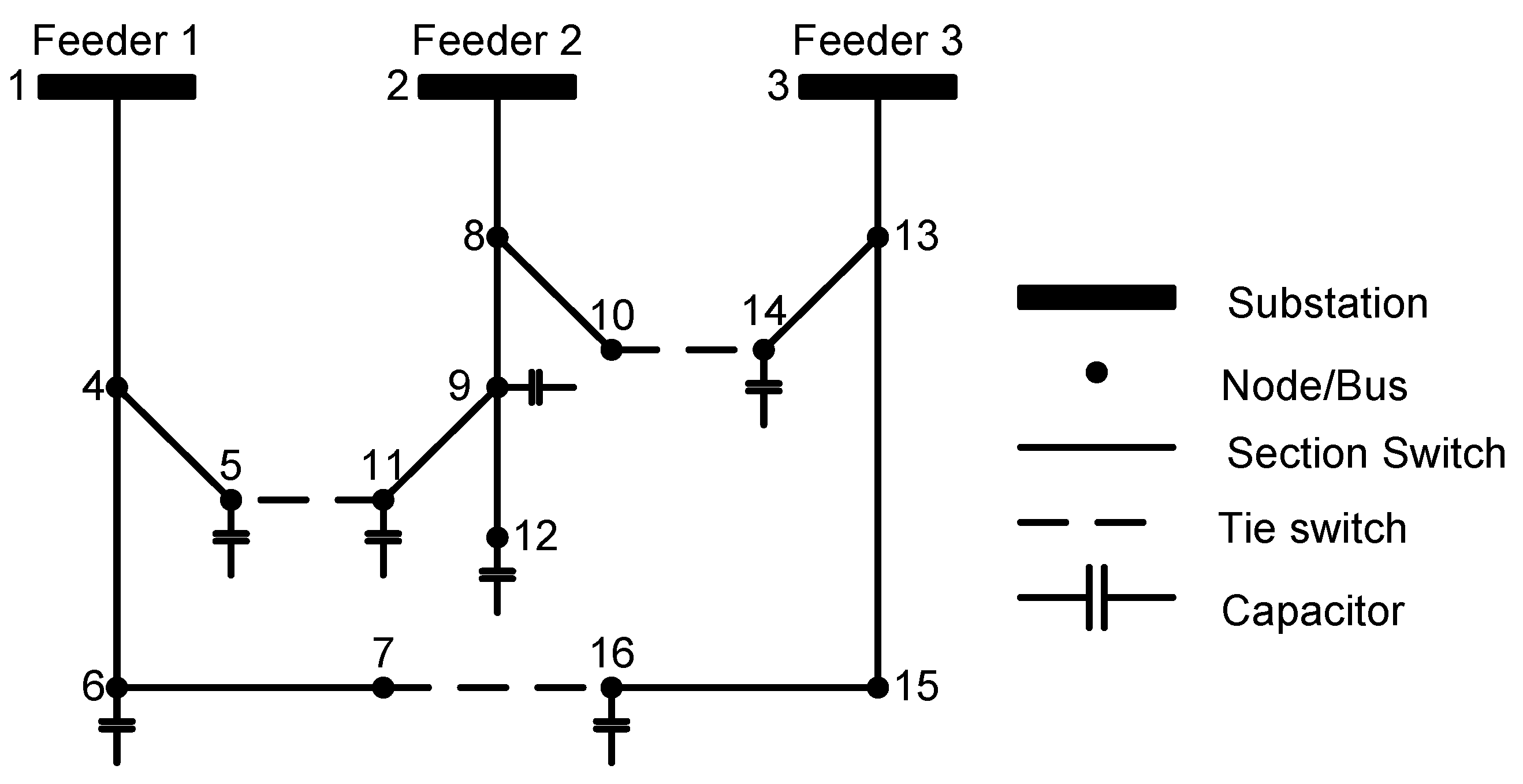
The research methodology consists of developing a DPSO method as described in Section 3 (Steps 1 to 15) to reduce real power loss and optimizing the load balancing index with higher capacity reserve in its branches and a network topology that is more resistant to overload. To demonstrate the methodology, three case studies of IEEE 16, 33, and 69 distribution systems are considered. One of the case studies (IEEE 16 bus) is described below. Figure 1 depicts a three-feeder, three-Tie switch, seven capacitors, and sixteen-node distribution network. Each solid line in this diagram represents a sectionalizing switch that is ordinarily closed, and each dashed line represents a tie switch that is normally open. If a malfunction upstream on feeder 1 considerably lowers its capacity, part of the loads linked to it must be transferred to the other two feeders. This reconfiguration must be done in such a way that the voltage limitations, line capacity, feeder capacity, and radiality constraints requirements are all met. Prolonging the life of the switching devices, this reconfiguration should need a limited number of switching operations.

2. Feeder Reconfiguration in a Distribution Network

The distribution network feeder reconfiguration problem has two objectives: to minimize real power loss and to maximize the load balancing index. The real power loss minimization problem is theoretically expressed as Equation (1). The total real power loss in a distribution system is expressed mathematically as the sum of the real component of the apparent power difference between the buses in the distribution system.

$${\mathrm{P}}_{\mathrm{loss}}={{\displaystyle \sum }}_{\begin{array}{c}\mathrm{j}=1\\ \mathrm{k}=1\\ \mathrm{j}\ne \mathrm{k}\end{array}}^{\mathrm{NB}}\mathrm{real}\left({\mathrm{V}}_{\mathrm{j}}\times {\mathrm{i}}_{\mathrm{jk}}{}^{*}-{\mathrm{V}}_{\mathrm{k}}\times {\mathrm{i}}_{\mathrm{jk}}{}^{*}\right) ,$$

(1)

where:

$\mathrm{j}$is the sending bus of line $\mathrm{j}-\mathrm{k}$,

$\mathrm{k}$is the receiving bus of line $\mathrm{j}-\mathrm{k}$,

${\mathrm{V}}_{\mathrm{j}},{ \mathrm{V}}_{\mathrm{k}}$are the sending and receiving end voltage of the line $\mathrm{j}-\mathrm{k}$, respectively,

${\mathrm{i}}_{\mathrm{jk}}{}^{*}$ is the conjugate of the current flow in line $\mathrm{j}-\mathrm{k}$,

${\mathrm{P}}_{\mathrm{loss}}$ is the total real power loss in the distribution system,

$\mathrm{NB}$ is the number of buses in the network, and

${\mathrm{V}}_{\mathrm{j}}\times {\mathrm{i}}_{\mathrm{jk}}{}^{*}={\mathrm{S}}_{\mathrm{j}\mathrm{k}}$ and ${\mathrm{V}}_{\mathrm{k}}\times {\mathrm{i}}_{\mathrm{jk}}{}^{*}={\mathrm{S}}_{\mathrm{k}\mathrm{j}}$.

The Load Balancing Index (LBI-sys) is mathematically expressed in Equation (2) (Baran and Wu, 1989). To keep the distribution network feeders as balanced as feasible, the load balancing index LBI-sys should be minimized.

$${\mathrm{LBI}}_{\mathrm{sys}}=\frac{1}{\mathrm{NL}}{{\displaystyle \sum }}_{\mathrm{l}=1}^{\mathrm{NL}}\frac{{\mathrm{S}}_{\mathrm{l}}}{{\mathrm{S}}_{\mathrm{l} \max }} ,$$

(2)

where:

$\mathrm{l}$ is the branch number of the line $\mathrm{j}-\mathrm{k}$,

${\mathrm{S}}_{\mathrm{l}}$ is the apparent power loss in the branch $\mathrm{l}$,

${\mathrm{S}}_{\mathrm{l} \max }$ is the power rating of branch $\mathrm{l}$,

${\mathrm{LBI}}_{\mathrm{sys}}$ is the load balance index of the network, and

$\mathrm{NL}$ is the number of branches in the distribution system.

Load balancing strives to optimize the use of network branches, to maximize branch capacity utilization, to avoid overloading a single branch, and to supply a load from other branches. A low load balancing index value suggests that the distribution system has more capacity reserve in its branches and that the network structure is more resistant to overload.

When the objectives of an optimization problem are incompatible, there is no single optimal solution but, rather, a set of solutions. Multi-objective optimization challenges can be mathematically expressed as shown in Equation (3).

$$\min \mathrm{f}\left(\mathrm{x}\right)=\left[{\mathrm{f}}_1\left(\mathrm{x}\right),{ \mathrm{f}}_2\left(\mathrm{x}\right), \dots ,{ \mathrm{f}}_{\mathrm{n}}\left(\mathrm{x}\right)\right],$$

(3)

subject to:

$${\mathrm{g}}_{\mathrm{j}}\left(\mathrm{x}\right)\le 0\hspace{1em}\hspace{1em} \mathrm{j}=1, 2, \dots , \mathrm{J} \hspace{1em}\hspace{1em}\left(\mathrm{inequality} \mathrm{constraint}\right),$$

$${\mathrm{h}}_{\mathrm{k}}\left(\mathrm{x}\right)=0\hspace{1em}\hspace{1em}\hspace{1em} \mathrm{k}=1, 2, \dots , \mathrm{K} \hspace{1em} \left(\mathrm{equality} \mathrm{constraint}\right),$$

$${\mathrm{x}}_{\mathrm{i}}{}^{\mathrm{L}}\le {\mathrm{x}}_{\mathrm{i}}\le {\mathrm{x}}_{\mathrm{i}}{}^{\mathrm{U}}\hspace{1em} \mathrm{i}=1, 2, \dots , \mathrm{I} \hspace{1em}\hspace{1em}\left(\mathrm{variables} \mathrm{limit}\right),$$

where:

$\mathrm{n}$is the number of objective functions,

${\mathrm{g}}_{\mathrm{j}}$and ${\mathrm{h}}_{\mathrm{k}}$are the inequality and equality constraints, respectively, and

$\mathrm{I}$, $\mathrm{J}$, and $\mathrm{K}$ are the number of decision variables, the number of inequality constraints, and the number of equality constraints, respectively,

Not all of the search space’s solutions are ideal. A set of optimal solutions is produced by a multi-objective optimization problem with competing objectives. As a result, the search space can be separated into two groups:

-

a set ${\mathrm{S}}_1$ of optimal solutions (non-dominated set) and

-

a set ${\mathrm{S}}_2$of non-optimal solutions (dominated set).

To discover the best solutions in the search space, the multi-objective optimization method employs the concept of dominance and non-dominance. Any two solutions in ${\mathrm{S}}_1$ are not dominated by each other, and any solution in ${\mathrm{S}}_1$ is dominated by at least one solution in ${\mathrm{S}}_1$.

Let us consider $\mathrm{u}=\left[{\mathrm{u}}_1,{ \mathrm{u}}_2, \dots ,{ \mathrm{u}}_{\mathrm{i}}\right]$and $\mathrm{v}=\left[{\mathrm{v}}_1,{ \mathrm{v}}_2, \dots ,{ \mathrm{v}}_{\mathrm{i}}\right]$, two solutions to the search space. $\mathrm{u}$ dominates $\mathrm{v}$ ($\mathrm{u}<\mathrm{v}$) if:

-

$\mathrm{u}$is no worse than $\mathrm{v}$ for all objectives, i.e., ${\mathrm{f}}_{\mathrm{i}}\left(\mathrm{u}\right)\le {\mathrm{f}}_{\mathrm{i}}\left(\mathrm{v}\right), \forall \mathrm{i}=1, 2, \dots , \mathrm{n}$, and

-

$\mathrm{u}$ is strictly better than $\mathrm{v}$ for at least one objective, i.e., ${\mathrm{f}}_{\mathrm{i}}\left(\mathrm{u}\right)<{\mathrm{f}}_{\mathrm{i}}\left(\mathrm{v}\right),$for at least one$\mathrm{i}\in \left\{1, 2, \dots , \mathrm{n}\right\}$.

Pareto-dominance is the notion discussed above. If there is no other solution $\mathrm{v}$ in the search space that is Pareto-optimal, then solution $\mathrm{u}$ is Pareto-optimal that ${\mathrm{f}}_{\mathrm{i}}\left(\mathrm{v}\right)<{\mathrm{f}}_{\mathrm{i}}\left(\mathrm{u}\right),$ for all the objectives of the problem. The set ${\mathrm{S}}_1$ of Pareto optimal (non-dominated) solutions is referred to as the Pareto-optimal set [14]. Equations (2) and (3), compute the load flow based on the optimal particle position to determine the personal best position in Step 5 of the developed DPSO algorithm.

3. Development of the Discrete Particle Swarm Optimization Method

Eberhart and Kennedy first proposed the Particle Swarm Optimization (PSO) technique in 1995. It is a stochastic search method that was inspired by the behavior of a flock of birds or a school of fish [15]. The binary PSO is an alternative to the canonical PSO. Kennedy and Eberhart [16] proposed it for the first time in 1997.

The following stages are used to develop the Discrete PSO-based solution technique for the multi-objective feeder reconfiguration problem:

Step 1: Read the distribution system network data, which includes the number of nodes, distribution lines, tie lines, bus type (Slack, PV, PQ), load data, generator data, and distribution line data.

Step 2: Set the binary PSO parameters, such as the acceleration coefficients c1 and c2; the minimum and maximum inertia weights (${\mathrm{w}}_{\min }$ and ${\mathrm{w}}_{\max }$); the particle velocity limits (${\mathrm{v}}_{\min }$and ${\mathrm{v}}_{\max }$); the number of particles (Np); the dimension of the search space (D); and the stopping criteria (maximum number of iterations ${\mathrm{t}}_{\max }$).

Step 3: Initialize the particle position, which is the binary coded representation of the distribution network’s section and tie-switches. The binary bit ones (1) and zeros (0) represent the section and tie switches, respectively. A particle represents a potential distribution network structure. A viable candidate solution is one that is practical (comply with the distribution network feeder reconfiguration constraints) topology of distribution networks.

The IEEE 16-bus distribution system is depicted in Figure 1, and its specifications are listed in

Table 1. The 16-bus distribution network is represented in binary (Bits).

Line No	1	2	3	4	5	6	7	8	9	10	11	12	13	14	15	16
Sending Bus	1	4	4	6	2	8	8	9	9	3	13	13	15	5	10	7
Receivingbus	4	5	6	7	8	9	10	11	12	13	14	15	16	11	14	16
Status	1	1	1	1	1	1	1	1	1	1	1	1	1	0	0	0

[17].

Table 1 contains the binary version of the 16-bus distribution system depicted in Figure 1. Lines 14, 15, and 16 of Table 1 indicate tie-switches with binary bit (status) zeros, and the remaining lines represent section switches with binary bit ones.

The location of a particle is a string of bits that represents the open or closed condition of the section and tie-switches in the distribution network. A conceivable particle in the 16-bus distribution system is symbolized by:

$${\mathrm{x}}_{\mathrm{i}}{}^{\mathrm{k}}=\left[1\hspace{1em}1\hspace{1em}1\hspace{1em}1\hspace{1em}1\hspace{1em}1\hspace{1em}1\hspace{1em}1\hspace{1em}1\hspace{1em}1\hspace{1em}1\hspace{1em}1\hspace{1em}1\hspace{1em}0\hspace{1em}0\hspace{1em}0\right],$$

where:

$\mathrm{i}$ is the particle number, and

$\mathrm{k}$ is the iteration number. $\mathrm{k}$is equal to $0$ for the initial particle position.

Step 4: Initialize the particle velocity, which reflects the likelihood that each bit in the particle’s position will change from open (0) to close (1) or from close (1) to open (0). Each particle in the search space moves at a distinct speed.

Equation (4) is used to compute the particle’s velocity.

$$\mathrm{velocity}\left(\mathrm{i},\mathrm{j}\right)={\mathrm{v}}_{\min }+\left({\mathrm{v}}_{\max }-{\mathrm{v}}_{\min }\right)\times \mathrm{rand},$$

(4)

where:

$\mathrm{i}$ is the particle number,

$\mathrm{j}$ is the index of the dimension of the search space,

$\mathrm{velocity}\left(\mathrm{i},\mathrm{j}\right)$ is the probability of the $\mathrm{j}$-bit of particle $\mathrm{i}$ to change its status from open to close or close to open,

${\mathrm{v}}_{\min }$ is the minimum velocity,

${\mathrm{v}}_{\max }$ is the maximum velocity, and

$\mathrm{rand}$ is a random number in the range $\left[0,1\right]$.

Step 5: Determine your personal best particle position. The original particle position is presumed to be the optimal particle position in this scenario. Then, using Equations (2) and (3), compute the load flow based on the optimal particle position and get the real power loss and load balancing index. A particle’s personal best position has two individual fitness values, which indicate the particle’s real power loss and the load balancing index. As a result, the fitness of a particular particle $\mathrm{i}$ is defined as follows:

$${\mathrm{fitness}}_{\mathrm{i}}=\left[\mathrm{fitness}{1}_{\mathrm{i}}, \mathrm{fitness}{2}_{\mathrm{i}}\right],$$

(5)

where:

${\mathrm{fitness}}_{\mathrm{i}}$ is the fitness of particle $\mathrm{i}$,

$\mathrm{fitness}1$ is the real power loss for the particle’s position, and

$\mathrm{fitness}2$ is the load balancing index for the particle’s position.

Step 6: From the set of particle best positions given in Step 5, determine the global best particle position. In this situation, the best particle position with the least amount of real power loss and the highest load balancing index value is the global best particle position.

Step 7: Compute the distribution network’s bus incidence matrix. The bus incidence matrix is used to determine whether or not a link exists between the two nodes. This aids in determining if the network topology is radial or not.

Begin the binary PSO iteration process by setting the iteration counter t to 1.

Step 8: After updating the bus incidence matrix for the proposed network topologies, check the topological constraints to see if all of the possible solutions match the topology criteria. This phase ensures that the real power loss and load balancing index are calculated only for distribution network topologies that are feasible.

Step 9: Using the Newton–Raphson load flow technique, determine the power flow in the distribution network. Then, using Equations (2) and (3), use the power flow results to determine the real power loss and load balancing index of each candidate network configuration.

Step 10: Update the particles’ personal bests in accordance with Equation (6).

$${\mathrm{Pbest}}_{\mathrm{i}}^{\mathrm{t}+1}=\{\begin{array}{cc}{\mathrm{x}}_{\mathrm{i}}^{\mathrm{t}+1},& \mathrm{if} \mathrm{fitness}{1}_{\mathrm{i}}^{\mathrm{t}+1}<{\mathrm{fitness}}_{\mathrm{Pbest}1\mathrm{i}}^{\mathrm{t}} \mathrm{and} \mathrm{fitness}{2}_{\mathrm{i}}^{\mathrm{t}+1}<{\mathrm{fitness}}_{\mathrm{Pbest}2\mathrm{i}}^{\mathrm{t}}\\ {\mathrm{Pbest}}_{\mathrm{i}}^{\mathrm{t}},& \mathrm{otherwise}\end{array},$$

(6)

where:

${\mathrm{Pbest}}_{\mathrm{i}}{}^{\mathrm{t}}$ is the personal best position of particle $\mathrm{i}$ at iteration $\mathrm{t}$,

${\mathrm{x}}_{\mathrm{i}}{}^{\mathrm{t}+1}$ is the position of particle $\mathrm{i}$ at iteration $\mathrm{t}+1$,

$\mathrm{fitness}{1}_{\mathrm{i}}{}^{\mathrm{t}+1}$ is the real power loss of particle $\mathrm{i}$ at iteration $\mathrm{t}+1$,

$\mathrm{fitness}{2}_{\mathrm{i}}{}^{\mathrm{t}+1}$ is the load balancing index of particle $\mathrm{i}$ at iteration $\mathrm{t}+1$,

${\mathrm{fitness}}_{\mathrm{Pbest}1}{{}_{\mathrm{i}}}^{\mathrm{t}}$ is the real power loss of ${\mathrm{Pbest}}_{\mathrm{i}}{}^{\mathrm{t}}$ at iteration $\mathrm{t}$, and

${\mathrm{fitness}}_{\mathrm{Pbest}2}{{}_{\mathrm{i}}}^{\mathrm{t}}$ is the load balancing index of ${\mathrm{Pbest}}_{\mathrm{i}}{}^{\mathrm{t}}$ at iteration $\mathrm{t}$.

Step 11: Update the global best in the swarm of particles as per Equation (7).

$${\mathrm{Gbest}}^{\mathrm{t}+1}=\{\begin{array}{cc}{\mathrm{Pbest}}_{\mathrm{i}}^{\mathrm{t}+1},& {\mathrm{if} \mathrm{fitness}}_{\mathrm{Pbest}1\mathrm{i}}^{\mathrm{t}+1}<{\mathrm{fitness}}_{\mathrm{Gbest}1}^{\mathrm{t}}{ \mathrm{and} \mathrm{fitness}}_{\mathrm{Pbest}2\mathrm{i}}^{\mathrm{t}+1}<{\mathrm{fitness}}_{\mathrm{Gbest}1}^{\mathrm{t}}\\ {\mathrm{Gbest}}^{\mathrm{t}},& \mathrm{otherwise}\end{array},$$

(7)

where:

${\mathrm{Gbest}}^{\mathrm{t}+1}$ is the global best solution of the swarm at iteration $\mathrm{t}+1$,

${\mathrm{fitness}}_{\mathrm{Gbest}1}{}^{\mathrm{t}}$ is the real power loss of $\mathrm{Gbest}$ at iteration $\mathrm{t}$, and

${\mathrm{fitness}}_{\mathrm{Gbest}2}{}^{\mathrm{t}}$ is the load balancing index of $\mathrm{Gbest}$ at iteration $\mathrm{t}$.

Step 12: Equation (9) is used to calculate the inertia weight, and Equation (8) is used to update the velocity of all particles.

$${\mathrm{v}}_{\mathrm{i}}{}^{\mathrm{k}+1}={\mathsf{\omega }\times \mathrm{v}}_{\mathrm{i}}{}^{\mathrm{k}}+\mathrm{c}1\times \mathrm{rand}1\times \left({\mathrm{Pbest}}_{\mathrm{i}}-{\mathrm{x}}_{\mathrm{i}}{}^{\mathrm{k}}\right)+\mathrm{c}2\times \mathrm{rand}2\times \left({\mathrm{Gbest}}_{\mathrm{i}}-{\mathrm{x}}_{\mathrm{i}}{}^{\mathrm{k}}\right),$$

(8)

where:

$\mathsf{\omega }$ is the inertia weight.

Equation (9) is used to compute the inertia weight:

$$\mathsf{\omega }={\mathsf{\omega }}_{\max }-\left(\frac{{\mathsf{\omega }}_{\max }-{\mathsf{\omega }}_{\min }}{{\mathrm{t}}_{\max }}\right)\times \mathrm{t} ,$$

(9)

where:

${\mathsf{\omega }}_{\max }$ is the maximum inertia weight,

${\mathsf{\omega }}_{\min }$ is the minimum inertia weight,

${\mathrm{t}}_{\max }$ is the maximum number of iterations, and

$\mathrm{t}$ is the iteration number.

Step 13: Update the position of the particles in accordance with Equation (10):

$${\mathrm{x}}_{\mathrm{i}}{}^{\mathrm{k}}=\{\begin{array}{c}1 \mathrm{if} \mathrm{r}<\mathrm{s}\mathrm{i}\mathrm{g}\left({\mathrm{v}}_{\mathrm{i}}{}^{\mathrm{k}}\right)\\ 0 \mathrm{i}\mathrm{f} \mathrm{r}\ge \mathrm{s}\mathrm{i}\mathrm{g}\left({\mathrm{v}}_{\mathrm{i}}{}^{\mathrm{k}}\right)\end{array},$$

(10)

where:

$\mathrm{r}$ is a uniformly distributed random number in the interval [0,1], and

$\mathrm{sig}$ is a sigmoid function defined by $\mathrm{sig}\left(\mathsf{\alpha }\right)=\frac{1}{1+{\mathrm{e}}^{-\mathsf{\alpha }}}$.

Step 14: Increase the binary PSO search process’s iteration count, and repeat steps 8 to 13 until the stopping condition (maximum number of iterations) is met.

Step 15: Print the outcomes of multi-objective optimization, such as the global best solution (optimal distribution network topology) and the accompanying fitness values (real power loss and load balancing index).

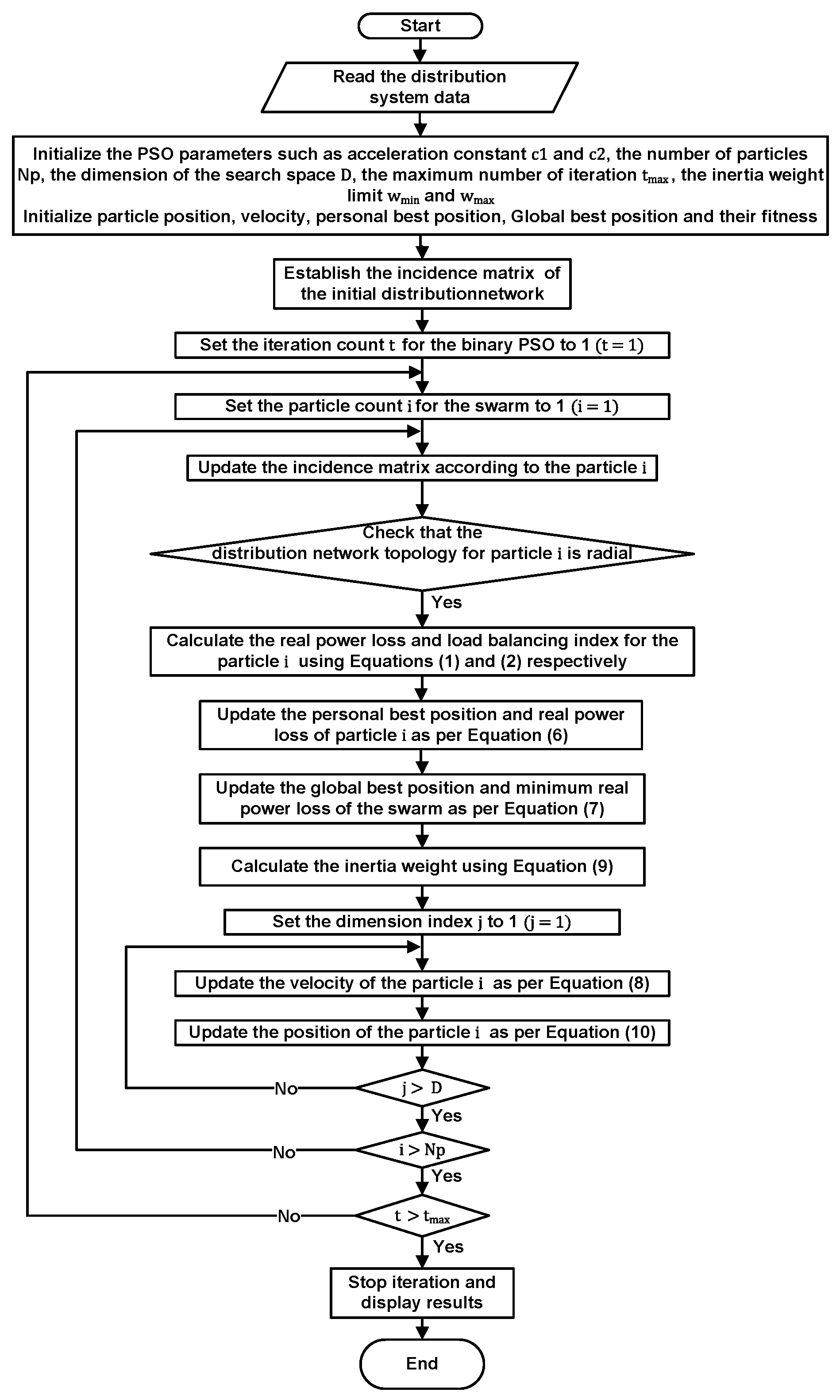
Equations (6) and (7) are used to update the personal best position and the global best position, respectively, to ensure that the final solution of the search process is not dominated by any other feasible solution in the search space. When the Binary PSO is utilized in practice, the particle velocity is limited to the interval [−4, 4] to avoid saturating the sigmoid function (Kennedy et al., 2001). Figure 2 depicts the flowchart for the BPSO solution algorithm for the multi-objective feeder reconfiguration problem.

4. The BPSO Solution Algorithm’s Results for the Multi-Objective Distribution Network Feeder Reconfiguration Problem

For three distribution systems, the developed multi-objective BPSO solution algorithm for the multi-objective distribution network feeder reconfiguration problem is examined. They are as follows:

-

IEEE 16 bus distribution system;

-

IEEE 33 bus distribution system; and

-

IEEE 69-bus distribution system.

Table 2. The simulation results of the 16-bus distribution system.

Algorithm		Developed BPSO Algorithm	ACO [18]	MINLP [19]	Refined GA [20]	Modified Tabu-Search [21]
Before reconfiguration	Tie switches	$14\hspace{1em}15\hspace{1em}16$	$14\hspace{1em}15\hspace{1em}16$	$14\hspace{1em}15\hspace{1em}16$	$14\hspace{1em}15\hspace{1em}16$	$14\hspace{1em}15\hspace{1em}16$
	Real power loss	$511.4029 \mathrm{kW}$	$511.4 \mathrm{kW}$	$511.44 \mathrm{kW}$	$511.4 \mathrm{kW}$	$511.4 \mathrm{kW}$
	Load Balancing index (LBI)	$2.9812\times {10}^{-3}$	−	−	−	−
	Minimum voltage	$0.9707 \mathrm{p.u.}$ $@ \mathrm{bus} 12$	$0.9707 \mathrm{p.u.}$ $@ \mathrm{bus} 12$	$0.9707 \mathrm{p.u.}$ $@ \mathrm{bus} 12$	$0.9707 \mathrm{p.u.}$ $@ \mathrm{bus} 12$	$0.9707 \mathrm{p.u.}$ $@ \mathrm{bus} 12$
After reconfiguration	Tie switches	$7\hspace{1em}8\hspace{1em}16$	$7\hspace{1em}8\hspace{1em}16$	$7\hspace{1em}8\hspace{1em}16$	$7\hspace{1em}8\hspace{1em}16$	$7 8 16$
	Real power loss	$466.0833 \mathrm{kW}$	$466.1 \mathrm{kW}$	$466.13 \mathrm{kW}$	$466.1 \mathrm{kW}$	$466.1 \mathrm{kW}$
	Real power loss reduction	$8.8618\%$	$8.858\%$	$8.856\%$	$8.858\%$	$8.858\%$
	Load Balancing index (LBI)	$2.7676\times {10}^{-3}$	−	−	−	−
	Load balance improvement	$7.166\%$	−	−	−	−
	Minimum voltage	$0.9693 \mathrm{p.u.}$	$0.9693 \mathrm{p.u.}$	$0.9693 \mathrm{p.u.}$	$0.9693 \mathrm{p.u.}$	$0.9693 \mathrm{p.u.}$
CPU Time		$0.36 \mathrm{s}$	−	−	−	−

,

Table 3. The simulation results of the 33-bus distribution system’s multi-objective feeder reconfiguration problem.

Algorithm		Developed BPSO Algorithm	Sequential Switch Opening Method [22]	Modified PSO [23]	HBMO [7]
Before reconfiguration	Tie switches	$33 34 35 36 37$	$33 34 35 36 37$	$33 34 35 36 37$	$33 34 35 36 37$
	Real power loss	$208.4322 \mathrm{kW}$	$202.05 \mathrm{kW}$	$202.6 \mathrm{kW}$	$208.15 \mathrm{kW}$
	Load Balancing Index (LBI)	$2.9812\times {10}^{-3}$	−	−	−
After reconfiguration	Tie switches	$7\hspace{1em}9\hspace{1em}14\hspace{1em}32\hspace{1em}37$	$7\hspace{1em}9\hspace{1em}14\hspace{1em}32\hspace{1em}37$	$7\hspace{1em}9\hspace{1em}14\hspace{1em}32\hspace{1em}37$	$7\hspace{1em}9\hspace{1em}14\hspace{1em}32\hspace{1em}37$
		$7\hspace{1em}9\hspace{1em}14\hspace{1em}28\hspace{1em}31$
		$7\hspace{1em}9\hspace{1em}14\hspace{1em}28\hspace{1em}32$
	Real power loss	$138.9105 \mathrm{kW}$	$139.21 \mathrm{kW}$	$139.5 \mathrm{kW}$	$139.53 \mathrm{kW}$
		$144.1694 \mathrm{kW}$
		$139.9645 \mathrm{kW}$
	Real power loss reduction	$33.3546\%$	$31.1012\%$	$31.1\%$	$31.14\%$
		$30.8315\%$
		$32.8489\%$
	Load Balancing Index (LBI)	$1.4503\times {10}^{-4}$	−	−	−
		$1.3487\times {10}^{-4}$
		$1.3751\times {10}^{-4}$
	Load balancing improvement	$29.2125\%$	−	−	−
		$34.1697\%$
		$32.88251\%$
	Minimum voltage	$0.9423 \mathrm{p.u.}$ $@ \mathrm{bus} 32$	$0.93796$ $@ \mathrm{bus} 32$	$0.9378 \mathrm{p.u.}$	$0.9378 \mathrm{p.u.}$
		$0.9239 \mathrm{p.u.}$ $@ \mathrm{bus} 32$
		$0.9413 \mathrm{p.u.}$ $@ \mathrm{bus}32$
CPU Time		~1.9 s	−	−	$~8 \mathrm{s}$

and Table 4 for the investigated distribution systems give a comparative examination of the distribution system before and after the feeder reconfiguration. The study is based on the real power loss, load balancing index, voltage profile, and change in distribution network structure.

4.1. Case Study 1: The IEEE 16-Bus Distribution System

The developed multi-objective BPSO method is utilized to determine the best network topology to minimize real power loss and load balancing index in a 16-bus distribution system. Table 2 compares the optimization outcomes for a 16-bus distribution system before and after feeder reconfiguration.

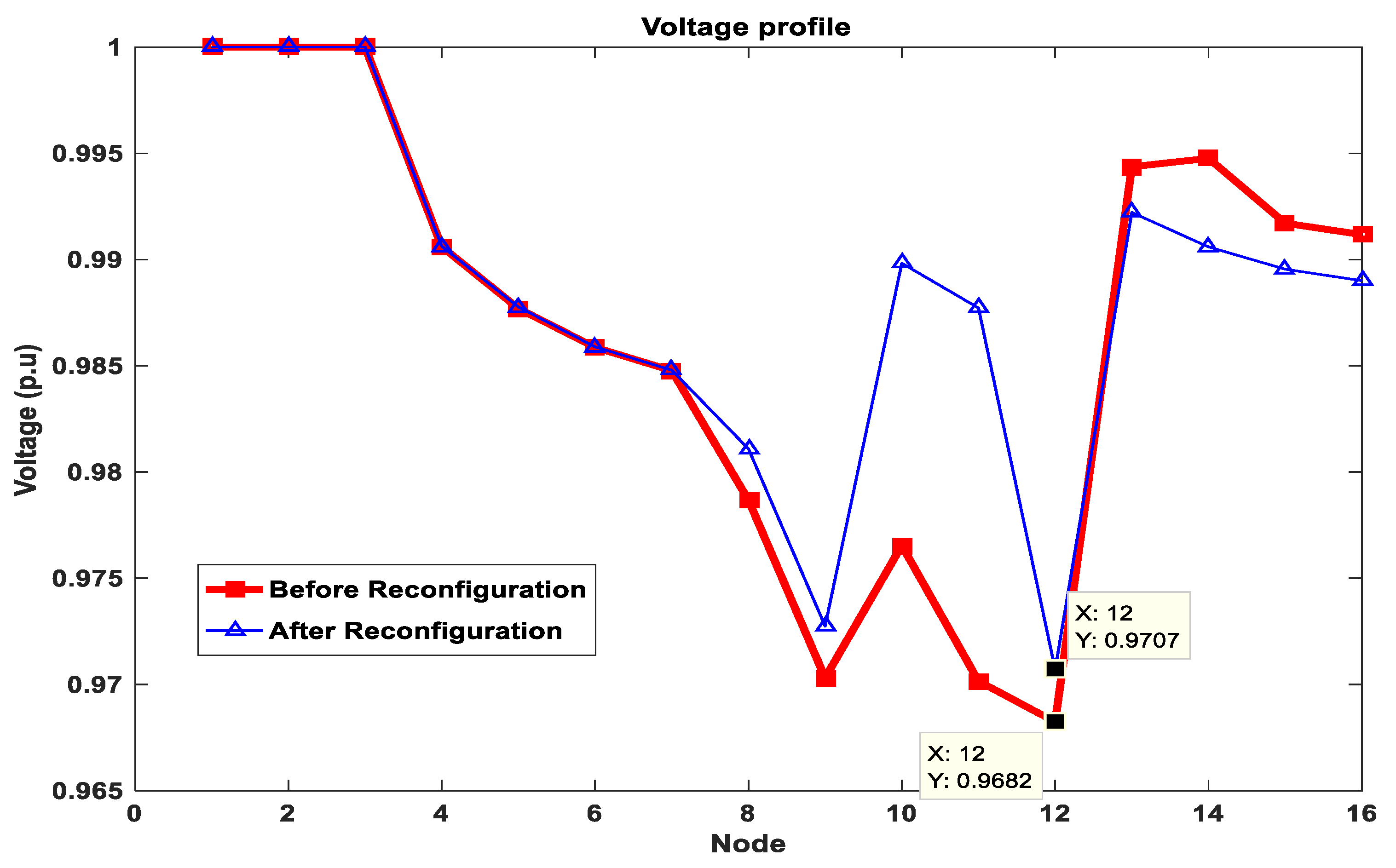
Before the feeder reconfiguration, the tie-lines are located at branch numbers 14, 15, and 16; however, after the feeder reconfiguration, the tie-lines are located at branch numbers 7, 8, and 16. This demonstrates that the created multi-objective BPSO algorithm successfully redesigned the distribution system and discovered its best network topology. The network architecture improvement reduced the real power loss and load balancing index of the 16-bus distribution system. Following the feeder reconfiguration, the distribution system’s real power loss is decreased to 468.3304 kW from 514.02932 kW, and the load balancing index is reduced to $2.7676\times {10}^{-3}$ from $2.9812\times {10}^{-3}$. In comparison to the initial distribution system solution, this optimization approach results in a real power loss reduction of roughly 8.89033 percent and an LBI improvement of 7.166 percent. As demonstrated in Figure 3, the adjustment in distribution network design improved the voltage profile. The minimum voltage at bus 12 before the feeder reconfiguration is 0.9682 p.u., and it improves to 0.9707 p.u. after the feeder reconfiguration.

4.2. Case Study 2: The IEEE 33-Bus Distribution System

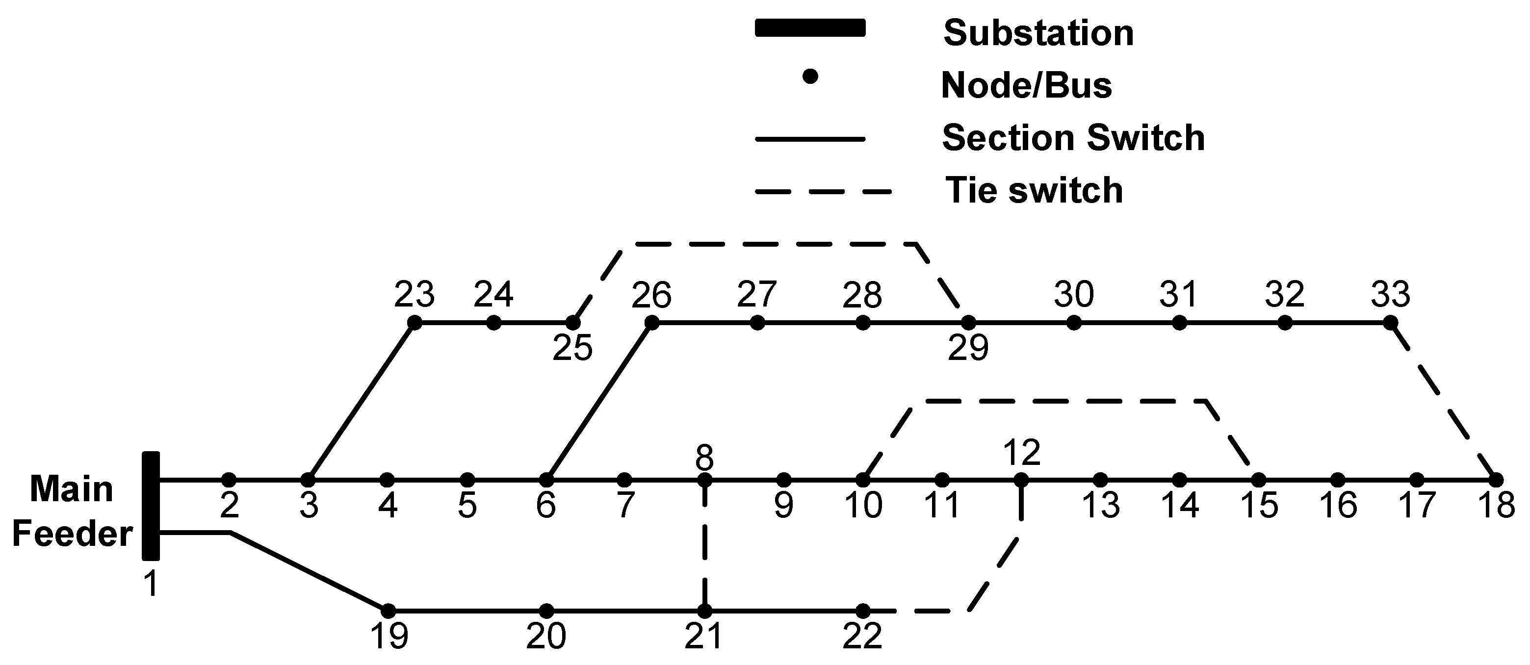
Figure 4 depicts the single line diagram of the 33-bus distribution system, and its specifications may be found in Baran and Wu (1989). Table 3 shows a comparison of the optimization outcomes of the 33-bus distribution system before and after feeder reconfiguration.

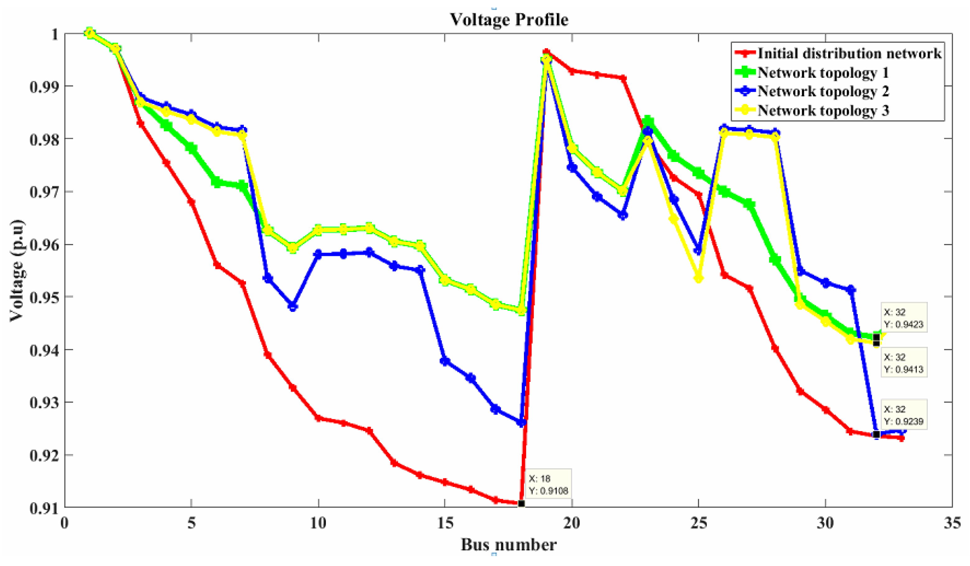
As a result, there are three Pareto-optimal or non-dominated network topology alternatives when using the devised multi-objective BPSO algorithm for optimal feeder reconfiguration of the 33-bus network. They are as follows:

-

Network topology 1: The tie switches for the 33-bus distribution system may be found at branches 7 (branch 7-8), 9 (branch 9–10), 14 (branch 14–15), 32 (branch 32–33), and 37 (branch 25–29). The real power loss for this network design is 138.9105 kW, and the load balancing index is $1.4503\times {10}^{-4}$. Compared to the baseline distribution system, this optimization method results in a real power loss reduction of roughly 33.3546 percent and an LBI improvement of 29.2125 percent. In the search space, network topology 1 has the lowest real power loss. As a result, network topology 1 outperforms all other proposed network topologies in terms of real power loss.

-

Network topology 2: The tie switches of the 33-bus distribution system are branches 7 (branch 7–8), 9 (branch 9–10), 14 (branch 14–15), 28 (branch 28–29), and 31 (branch 31–32). The real power loss for this network design is 144.1694 kW and the load balancing index is $1.3487\times {10}^{-4}$. Compared to the original distribution system, this optimization method results in an actual power loss reduction of roughly 30.8315 percent and an LBI improvement of 34.1697 percent. Network topology 2 has the lowest load balancing index in the search space. As a result, network topology 2 is non-dominant in the search space in terms of load balancing index.

-

Network topology 3: The tie switches of the 33-bus distribution system are branches 7 (branch 7–8), 9 (branch 9–10), 14 (branch 14–15), 28 (branch 28–29), and 32 (branch 32–33). The real power loss for this network design is 139.9645 kW and the load balancing index is $1.3751\times {10}^{-4}$. Compared to the baseline distribution system, this optimization method results in a real power loss reduction of roughly 32.8489 percent and an LBI improvement of 32.88251 percent.

The real power loss of network topology 3 (139.9645 kW) is more than that of network topology 1 (138.9105 kW), and the load balancing index of network topology 1 ($1.4503\times {10}^{-4}$) is greater than that of network topology 3. Similarly, the real power loss of network topology 2 (144.1694 kW) is more than that of network topology 3 (139.9645 kW), and the load balancing index of network topology 2 ($1.3751\times {10}^{-4}$) is lower than that of network topology 3. As a result, the solution network topologies 1, 2, and 3 are Pareto-optimal and non-dominated with regard to each other, according to the Pareto-optimality criterion described in Section 2.

However, as with most real-world situations, the solution to the multi-objective problem requires only one network topology. As a result, higher-level knowledge is necessary to divide the Pareto-optimal network topologies. The voltage profile is employed as the higher-level information in this scenario. Figure 5 depicts the voltage profiles of the non-dominated solutions. Figure 5 shows that network configuration 3 has a higher voltage profile than network topologies 1 and 2. As a result, despite the fact that network topology 3 has a lower minimum voltage (0.9413 p.u.) than network topology 1 (0.9423 p.u.), network topology 3 emerges as the recommended optimal solution of the multi-objective feeder reconfiguration problem for the 33-bus distribution system.

4.3. Case Study 3: The IEEE 69-Bus Distribution System

Figure 6 depicts a single line diagram of the 69-bus distribution system. The parameters of the 69-bus distribution network are given in [24].

Table 4 presents a comparison of the optimization outcomes of the 69-bus distribution system before and after feeder reconfiguration. The application of the multi-objective feeder reconfiguration method to the 69-bus distribution system yields a number of non-dominated solution network topologies.

Table 4. Simulation findings for the 69-bus distribution system’s multi-objective feeder reconfiguration problem.

Algorithm		Developed BPSO Algorithm		Harmony Search [25]	Selective PSO [26]
Before reconfiguration	Tie switches	$69 70 71 72 73$		$69 70 71 72 73$	$69 70 71 72 73$
	Real power loss	$224.9804 \mathrm{kW}$		$225 \mathrm{kW}$	$224.96 \mathrm{kW}$
	Load Balancing Index (LBI)	$2.0488\times {10}^{-4}$		−	−
After reconfiguration	Tie switches	$\mathrm{Set} 1$	$\mathrm{Set} 2$	$13\hspace{1em}18\hspace{1em}56\hspace{1em}61\hspace{1em}69$	$14\hspace{1em}56\hspace{1em}63\hspace{1em}69\hspace{1em}70$
		$14\hspace{1em}55\hspace{1em}61\hspace{1em}69\hspace{1em}70$ $14\hspace{1em}56\hspace{1em}61\hspace{1em}69\hspace{1em}70$ $14\hspace{1em}57\hspace{1em}61\hspace{1em}69\hspace{1em}70$ $14\hspace{1em}58\hspace{1em}61\hspace{1em}69\hspace{1em}70$	$12\hspace{1em}18\hspace{1em}56\hspace{1em}61\hspace{1em}69$ $12\hspace{1em}18\hspace{1em}57\hspace{1em}61\hspace{1em}69$ $12\hspace{1em}18\hspace{1em}58\hspace{1em}61\hspace{1em}69$ $12\hspace{1em}19\hspace{1em}55\hspace{1em}61\hspace{1em}69$ $12\hspace{1em}20\hspace{1em}55\hspace{1em}61\hspace{1em}69$ $12\hspace{1em}20\hspace{1em}57\hspace{1em}61\hspace{1em}69$
	Real power loss	$98.5952 \mathrm{kW}$	$101.2961 \mathrm{kW}$	$99.35 \mathrm{kW}$	$98.9824 \mathrm{kW}$
	Real power loss reduction	$56.1761\%$	$54.9756\%$	$55.85\%$	$~56\%$
	Load Balancing Index (LBI)	$1.5479\times {10}^{-4}$	$1.5295\times {10}^{-4}$	−	−
	Load balancing improvement	$35.6355\%$	$36.4006\%$	−	−
	Minimum voltage	$0.9495 \mathrm{p.u.}$ $@ \mathrm{bus} 61$	$0.9495 \mathrm{p.u.}$ $@ \mathrm{bus} 61$	$0.9428 \mathrm{p.u.}$ $@ \mathrm{bus} 63$	−
CPU Time		$~12 \mathrm{s}$	$~12 \mathrm{s}$	−	−

Table 4. Simulation findings for the 69-bus distribution system’s multi-objective feeder reconfiguration problem.

Algorithm		Developed BPSO Algorithm		Harmony Search [25]	Selective PSO [26]
Before reconfiguration	Tie switches	$69 70 71 72 73$		$69 70 71 72 73$	$69 70 71 72 73$
	Real power loss	$224.9804 \mathrm{kW}$		$225 \mathrm{kW}$	$224.96 \mathrm{kW}$
	Load Balancing Index (LBI)	$2.0488\times {10}^{-4}$		−	−
After reconfiguration	Tie switches	$\mathrm{Set} 1$	$\mathrm{Set} 2$	$13\hspace{1em}18\hspace{1em}56\hspace{1em}61\hspace{1em}69$	$14\hspace{1em}56\hspace{1em}63\hspace{1em}69\hspace{1em}70$
		$14\hspace{1em}55\hspace{1em}61\hspace{1em}69\hspace{1em}70$ $14\hspace{1em}56\hspace{1em}61\hspace{1em}69\hspace{1em}70$ $14\hspace{1em}57\hspace{1em}61\hspace{1em}69\hspace{1em}70$ $14\hspace{1em}58\hspace{1em}61\hspace{1em}69\hspace{1em}70$	$12\hspace{1em}18\hspace{1em}56\hspace{1em}61\hspace{1em}69$ $12\hspace{1em}18\hspace{1em}57\hspace{1em}61\hspace{1em}69$ $12\hspace{1em}18\hspace{1em}58\hspace{1em}61\hspace{1em}69$ $12\hspace{1em}19\hspace{1em}55\hspace{1em}61\hspace{1em}69$ $12\hspace{1em}20\hspace{1em}55\hspace{1em}61\hspace{1em}69$ $12\hspace{1em}20\hspace{1em}57\hspace{1em}61\hspace{1em}69$
	Real power loss	$98.5952 \mathrm{kW}$	$101.2961 \mathrm{kW}$	$99.35 \mathrm{kW}$	$98.9824 \mathrm{kW}$
	Real power loss reduction	$56.1761\%$	$54.9756\%$	$55.85\%$	$~56\%$
	Load Balancing Index (LBI)	$1.5479\times {10}^{-4}$	$1.5295\times {10}^{-4}$	−	−
	Load balancing improvement	$35.6355\%$	$36.4006\%$	−	−
	Minimum voltage	$0.9495 \mathrm{p.u.}$ $@ \mathrm{bus} 61$	$0.9495 \mathrm{p.u.}$ $@ \mathrm{bus} 61$	$0.9428 \mathrm{p.u.}$ $@ \mathrm{bus} 63$	−
CPU Time		$~12 \mathrm{s}$	$~12 \mathrm{s}$	−	−

The non-dominated solutions are divided into two categories:

-

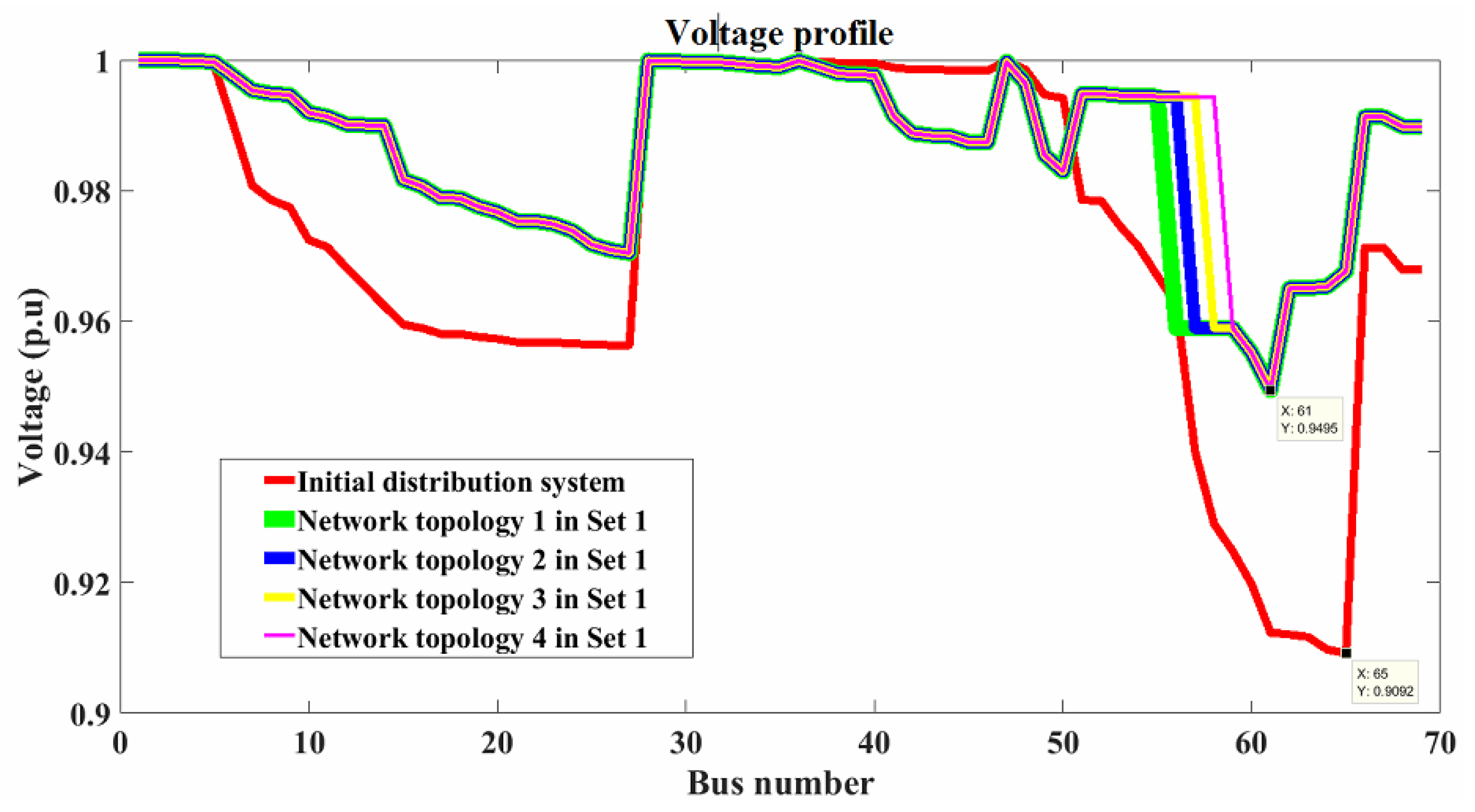
Set 1 is a collection of solution network topologies with a total power loss of 98.5952 kW and a load balancing index of $1.5479\times {10}^{-4}$. Compared to the initial distribution system, these optimization techniques result in an actual power loss reduction of roughly 56.1761 percent and an LBI improvement of 35.6355 percent.

-

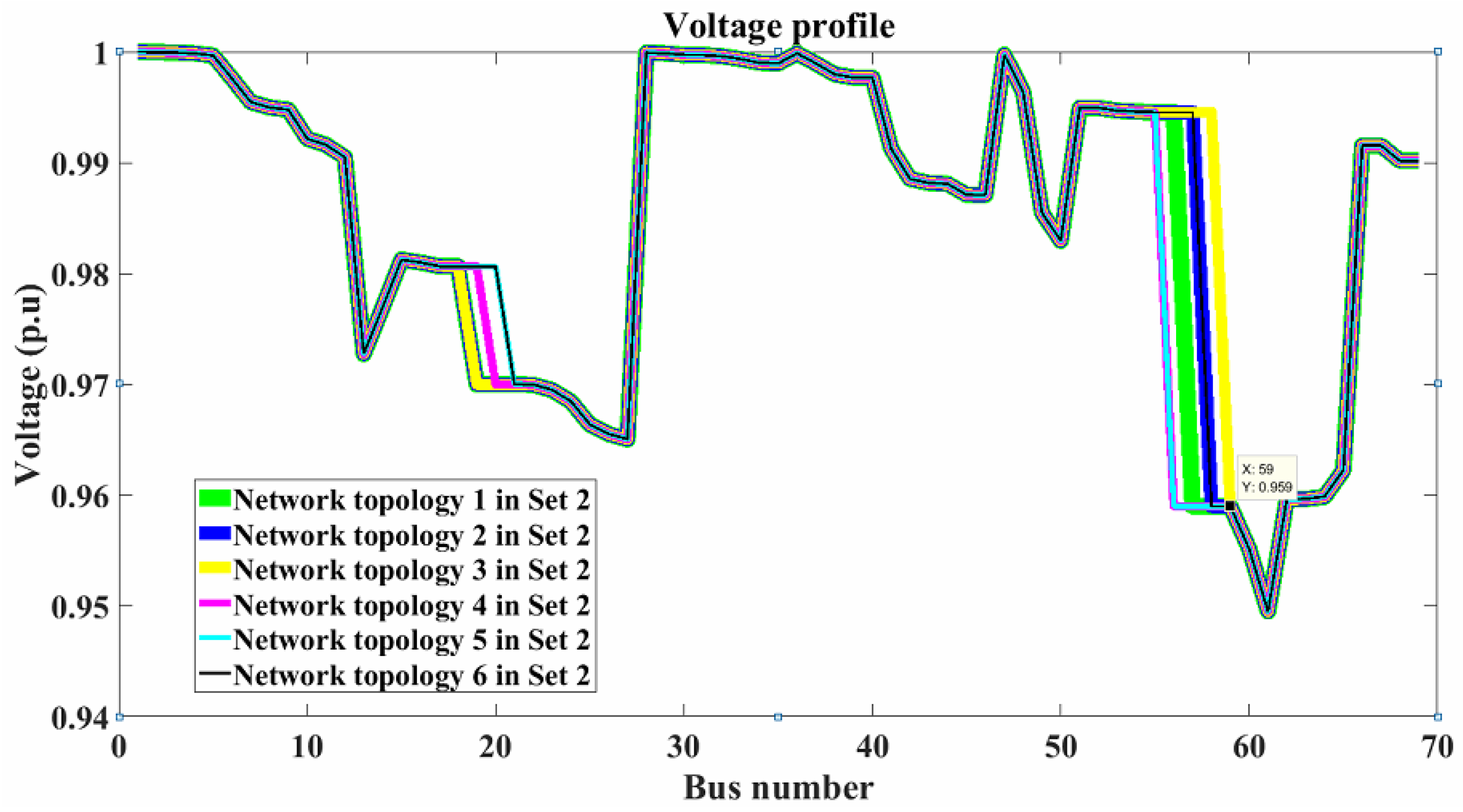
Set 2 is a collection of solution network topologies with a real power loss of 101.2961 kW and a load balancing index of $1.5295\times {10}^{-4}$. Compared to the initial distribution system, these optimization techniques result in an actual power loss reduction of roughly 54.9756 percent and an LBI improvement of 36.4006 percent.

Any solution network topology in Set 1 has a lower real power loss but a greater load balancing index than any solution network topology in Set 2. As a result, the solution network topologies in the two sets are Pareto-optimal in relation to one another. Given that the solution to the multi-objective problem requires just one network topology, the voltage profile is utilized to select the best optimal network topology from the two sets. Figure 7 and Figure 8 depict the voltage profiles of the network topologies in Sets 1 and 2. Figure 7 and Figure 8 show that the solution network topologies in Set 1 have a better voltage profile than those in Set 2. Furthermore, in Figure 7, the solution network architecture 4 from Set 1 has the best voltage profiles. As a result, the optimal solution of the multi-objective feeder reconfiguration problem for the 69-bus distribution system is solution network topology 4 from Set 1.

5. Discussion on the Comparison of the Developed BPSO Results with the Literature

It is difficult to compare the results of the developed multi-objective BPSO algorithm to the literature because no literature works have been discovered that consider distribution network feeder reconfiguration for real power loss minimization and load balancing as a multi-objective optimization problem. Refs. [27,28] developed various algorithms for solving the distribution network feeder reconfiguration problem for actual power loss minimization and load balancing. However, the authors saw the two aims as non-conflicting, and, as a result, the proposed algorithms were single-objective algorithms designed to minimize real power loss. Nonetheless, the produced BPSO results are compared to the literature in Table 2, Table 3 and Table 4 for the 16-bus, 33-bus, and 69-bus systems, respectively. The comparison study demonstrates that, when only the real power minimization aim is considered, the results of the developed BPSO algorithm are compatible with those of the literature, and the developed BPSO method achieves a greater real power loss reduction than the literature.

6. Conclusions

The purpose of this paper was to offer a novel Binary Particle Swarm Optimization algorithm solution to the multi-objective distribution network feeder reconfiguration problem. The goal of the multi-objective distribution network feeder reconfiguration problem was to minimize real power loss while also optimizing load balancing in the distribution network. To determine the best distribution system topology, the multi-objective feeder reconfiguration algorithm employs the Pareto-optimality principle. The performance of the developed BPSO algorithm was tested using the IEEE 16-bus, 33-bus, and 69-bus distribution systems. The simulation findings demonstrated:

-

For the analyzed 16-bus, 33-bus, and 69-bus distribution systems, the developed BPSO algorithm provides an optimal solution network topology to the multi-objective feeder reconfiguration problem.

-

The aims of real power loss minimization and load balancing are diametrically opposed. They may appear to be non-conflicting, depending on the loads, parameters, and distribution system design, as seen with the 16-bus distribution system.

Future research will evaluate the performance of the created BPSO algorithm in resolving distribution network feeder reconfiguration problems for a real-world utility network.

References

- Liu, C.; Lee, S.; Vu, K. Loss minimization of distribution feeders: Optimality and algorithms. IEEE Trans. Power Deliv. 1989, 4, 1281–1289. [Google Scholar] [CrossRef]
- Krishnamurthy, S.; Tzoneva, R.; Apostolov, A. Method for a Parallel Solution of a Combined Economic Emission Dispatch Problem. Electr. Power Compon. Syst. 2017, 45, 393–409. [Google Scholar] [CrossRef]
- Nguyen, T.T.; Nguyen, T.T. An improved cuckoo search algorithm for the problem of electric distribution network reconfiguration. Appl. Soft Comput. 2019, 84, 105720. [Google Scholar] [CrossRef]
- Enacheanu, B.; Bienia, W.; Devaux, O.; Caire, R.; Raison, B.; HadjSaid, N. Radial network reconfiguration using Genetic Algorithm based on the Matroid theory. IEEE Trans. Power Syst. 2008, 23, 186–195. [Google Scholar] [CrossRef]
- Jin, X.; Zhao, J.; Sun, Y.; Li, K.; Zhang, B. Distribution network reconfiguration for load balancing using binary particle swarm optimization. In Proceedings of the 2004 International Conference on Power System Technology (PowerCon 2004), Singapore, 21–24 November 2004; IEEE: Singapore, 2004; pp. 507–510. [Google Scholar]
- Hu, Z.; He, X.; Gao, Y.; Liu, D. Distribution network reconfiguration based on ant colony system algorithm. In Proceedings of the 2008 3rd IEEE Conference on Industrial Electronics and Applications, Singapore, 3–5 June 2008; pp. 2470–2474. [Google Scholar]
- Niknam, T. An efficient multi-objective HBMO algorithm for distribution feeder reconfiguration. Expert Syst. Appl. 2011, 38, 2878–2887. [Google Scholar] [CrossRef]
- Gebru, Y.; Bitew, D.; Aberie, H.; Gizaw, K. Performance enhancement of radial distribution system using simultaneous network reconfiguration and switched capacitor bank placement. Cogent Eng. 2021, 8, 1897929. [Google Scholar] [CrossRef]
- ElDesouky, A.; Reyad, E.; Mahmoud, G. Implementation of boolean PSO for service restoration using distribution network reconfiguration simultaneously with distributed energy resources and capacitor banks. Int. J. Renew. Energy Res. 2020, 10, 354–365. [Google Scholar]
- Wu, W.; Tsai, M. Feeder Reconfiguration Using Binary Coding Particle Swarm Optimization. Int. J. Control Autom. Syst. 2008, 6, 488–494. [Google Scholar]
- Muhammad, M.A.; Mokhlis, H.; Naidu, K.; Amin, A.; Franco, J.F.; Othman, M. Distribution Network Planning Enhancement via Network Reconfiguration and DG Integration Using Dataset Approach and Water Cycle Algorithm. J. Mod. Power Syst. Clean Energy 2020, 8, 86–93. [Google Scholar] [CrossRef]
- Helmi, A.M.; Carli, R.; Dotoli, M.; Ramadan, H.S. Efficient and Sustainable Reconfiguration of Distribution Networks via Metaheuristic Optimization. IEEE Trans. Autom. Sci. Eng. 2021, 19, 82–98. [Google Scholar] [CrossRef]
- Djiepkop, N. Feeder Reconfiguration Scheme with Integration of Renewable Energy Sources Using a Particle Swarm Optimisation Method. Master’s Thesis, Electrical, Cape Peninsula University of Technology, Cape Town, South Africa, 2018. [Google Scholar]
- Caramia, M.; Dell’Olmo, P. Multi-Objective Management in Freight Logistics: Increasing Capacity, Service Level and Safety with Optimization Algorithms; Springer: London, UK, 2014. [Google Scholar]
- Eberhart, R.; Kennedy, J. A new optimizer using particle swarm theory. In Proceedings of the MHS’95, the Sixth International Symposium on Micro Machine and Human Science, Nagoya, Japan, 4–6 October 1995; Institute of Electrical and Electronics Engineers (IEEE): New York, NY, USA, 1995; pp. 39–43. [Google Scholar]
- Kennedy, J.; Eberhart, R.C. A discrete binary version of the particle swarm algorithm. In Proceedings of the Computational Cybernetics and Simulation 1997 IEEE International Conference on Systems, Man, and Cybernetics, Orlando, FL, USA, 12–15 October 1997; Volume 5, pp. 4104–4108. [Google Scholar]
- Civanlar, S.; Grainger, J.; Yin, H.; Lee, S. Distribution feeder reconfiguration for loss reduction. IEEE Trans. Power Deliv. 1988, 3, 1217–1223. [Google Scholar] [CrossRef]
- Su, C.-T.; Chang, C.-F.; Chiou, J.-P. Distribution network reconfiguration for loss reduction by ant colony search algorithm. Electr. Power Syst. Res. 2005, 75, 190–199. [Google Scholar] [CrossRef]
- de Oliveira, L.W.; de Oliveira, E.J.; Gomes, F.V.; Silva, I.C.; Marcato, A.L.; Resende, P.V. Artificial Immune Systems applied to the reconfiguration of electrical power distribution networks for energy loss minimization. Int. J. Electr. Power Energy Syst. 2014, 56, 64–74. [Google Scholar] [CrossRef]
- Zhu, J. Optimal reconfiguration of electrical distribution network using the refined genetic algorithm. Electr. Power Syst. Res. 2002, 62, 37–42. [Google Scholar] [CrossRef]
- Abdelaziz, A.Y.; Mohamed, F.M.; Mekhamer, S.F.; Badr, M.A.L. Distribution system reconfiguration using a modified Tabu Search algorithm. Electr. Power Syst. Res. 2010, 80, 943–953. [Google Scholar] [CrossRef]
- Singh, S.P.; Raju, G.S.; Rao, G.K.; Afsari, M. A heuristic method for feeder reconfiguration and service restoration in distribution networks. Int. J. Electr. Power Energy Syst. 2009, 31, 309–314. [Google Scholar] [CrossRef]
- Abdelaziz, A.Y.; Mohammed, F.M.; Mekhamer, S.F.; Badr, M.A.L. Distribution Systems Reconfiguration using a modified particle swarm optimization algorithm. Electr. Power Syst. Res. 2009, 79, 1521–1530. [Google Scholar] [CrossRef]
- Savier, J.S.; Das, D. Impact of Network Reconfiguration on Loss Allocation of Radial Distribution Systems. IEEE Trans. Power Deliv. 2007, 22, 2473–2480. [Google Scholar] [CrossRef]
- Rao, R.S.; Ravindra, K.; Satish, K.; Narasimham, S.V.L. Power Loss Minimization in Distribution System Using Network Reconfiguration in the Presence of Distributed Generation. IEEE Trans. Power Syst. 2013, 28, 317–325. [Google Scholar] [CrossRef]
- Khalil, T.; Gorpinich, A. Reconfiguration for Loss Reduction of Distribution Systems Using Selective Particle Swarm Optimization. Int. J. Multidiscip. Sci. Eng. 2012, 3, 16–21. [Google Scholar]
- Baloch, Z. A new nonlinear constructive method for loss reduction and load balancing in radial distribution network reconfiguration. Eur. Sci. J. 2013, 9, 93–98. [Google Scholar]
- Baran, M.E.; Wu, F.F. Network reconfiguration in distribution systems for loss reduction and load balancing. IEEE Trans. Power Deliv. 1989, 4, 1401–1407. [Google Scholar] [CrossRef]
Figure 1.
The IEEE 16-bus distribution system.
Figure 2.
The developed Discrete PSO algorithm for the multi-objective distribution network feeder reconfiguration problem.
Figure 3.
The voltage profile of the 16-bus network before and after feeder reconfiguration.
Figure 4.
The 33-bus distribution system.
Figure 5.
The optimal network topologies’ voltage profiles for the 33-bus distribution system.
Figure 6.
The 69-bus distribution system.
Figure 7.
Voltage profiles of optimum network topologies for the 69-bus distribution system in Set 1.
Figure 8.
Voltage profiles of optimum network topologies for the 69-bus distribution system in Set 2.