
Hybrid Finite Element Method to Thermo-Elastic Interactions in a Piezo-Thermo-Elastic Medium under a Fractional Time Derivative Model


Nonlinear Analysis and Applied Mathematics Research Group (NAAM), Department of Mathematics, King Abdulaziz University, Jeddah 21589, Saudi Arabia
Mathematics 2022, 10(4), 650; https://0-doi-org.brum.beds.ac.uk/10.3390/math10040650
Submission received: 27 January 2022
/
Revised: 11 February 2022
/
Accepted: 15 February 2022
/
Published: 19 February 2022
(This article belongs to the Special Issue Analytical and Computational Mechanics of Advanced Materials and Functional Structures)
Abstract
:In this work, the effect of the fractional time derivative on the piezo-thermo-elastic medium is studied, using the hybrid Laplace transform and finite element methods (LFEM). The generalized fractional piezoelectric–thermoelastic basic equations for piezo-thermo-elastic medium are formulated. The Laplace transforms are used for the time derivatives, and the finite element method is used to discretize for the space derivatives. The inversions process is performed using the Stehfest numerical technique. The finite element approach is used to obtain the solutions of complex coupled formulations of this problem. The effects of fractional time derivative and thermal relaxation time on piezoelectric–thermoelastic mediums are studied. It can be seen from the distribution that the thermal-induced displacement, the temperature and the stress of the medium increase at a high fractional parameter.
1. Introduction
Recently, the problem of heat transfer in piezoelastic medium has been investigated by many researchers. Piezoelectricity undergoes mechanical stress when applied to solid samples, e.g., crystals, ceramics, and biomaterial such as bone, DNA, and other proteins. Piezoelectricity is comprehended as a linearly electro-mechanical interaction of a mechanical nature, and an electric case in crystal materials with no symmetrical obverse. Piezoelectricity is a changeful process, in that material exhibits a direct piezoelectric effect (the inner generation of electric charges produced due to mechanical forces), and it also exhibits reversible piezoelectricity (the inner generation of mechanical strain produced due to the electric field). Piezoelectricity can be investigated from lead zirconate titanate crystals when their static structure is distorted by approximately 0.1% of the original dimension. On the contrary, applying an exterior electric field on the same crystals will change 0.1% of their static dimension. Reverse piezoelectricity can be used to produce ultrasonic waves of sound. The piezoelectric effect is used in a large area of applications, for example, producing and detecting sound, high voltages, electronic frequency generation, micro-balances, to drive an ultrasonic nozzle, or the ultra-fine centering of an optical assembly. Moreover, it is the base of many scientific instruments with atomic resolution. Generalized thermoelastic theories have been proposed to overcome the limitations of classical coupling thermo-elasticity [1], in which heat travels at an infinite velocity. These models introduce time lags into the diffusion-types parabolic basic formulation of classical coupled thermo-elasticity, and transform them into wave-types hyperbolic equations. We observe that this finite wave-types heat propagation speed offers a more physically accommodating behavior [2,3]. Two of the most popular models are the Lord–Shulman model (LS model) [4] and the Green and Lindsay model (GL model) [5]. In the Lord and Shulman theory, the Fourier thermal conduction law is modulated by introducing a thermal delay time in the line of the Maxwell Cattaneo law. The Green and Lindsay model uses two thermal-delay time parameters and introduces the rate of temperature change into the stress–strain (Duhamel–Neumann relationship) and strain–entropy relationships. Other generalized thermoelastic models in the literature include the theory of Green–Naghdi (G-N) [6,7], which proposed another three generalized thermoelastic theories by modifying the energy equation, subsequently labelled by G-N I, G-N II and G-N III. Marin [8] studied the domain of influence theory for micro-stretch elastic material. Othman et al. [9] studied the novel models of a plane wave of two-temperature fiber-reinforced thermo-elastic material under the effect of gravity with three-phase-lag models. Marin [10] presented a partition of energy in micro-stretch thermoelastic bodies. Many works concerning the phenomenon of wave propagations in piezoelectric structure have been carried out by Cheng and Sun [10]. He et al. [11] used the Laplace transformation and its numerical inversions to study the generalized thermo-piezoelectric problem under one relaxation time due to moving heating sources. Akbarzadeh et al. [12] investigated the thermo-piezoelectric analysis of function-graded piezoelectric mediums. Ma and He [13] investigated the dynamics responses of a generalized piezo-electric-thermoelasticity problem under the fractional time derivative of the thermoelastic model. Saeed and Abbas [14] studied the effect of the nonlocal thermo-elastic model in thermo-elastic nanoscale materials. Guha and Singh [15] studied the reflections/transmissions of plane waves in composite half-spaces reinforced with rotating piezothermal elasticity fibers, initially stressed and imperfectly linked. Ragab et al. [16] studied the thermo-elastic piezo-electric fixed rod exposed to axial moving heating sources under DPL model. Biswas [17] studied the surface wave in piezo-thermo-elastic’s transverse isotropic layer lying over piezo-thermo-elastic’s transverse isotropic plane. Yang et al. [18] investigated the analysis of a composite piezoelectric semi-conductor cylindrical shell under the thermal loading. Singh, et al. [19] studied the shear wave in a piezo-fiber-reinforced poroelastic composites structure with sandwiched a functionally graded buffer layer: this is the power series approach. Serpilli et al. [20] disccused the higher order interface condition for piezoelectrics’ spherical hollow composite: these are asymptotic approaches and transfer matrix homogenization methods. Most deformation problems can be analytically solved using Laplace–Fourier transformation techniques, but finding the inversions of these approaches is quite difficult. To obviate these complications, the finite element scheme is chosen for time-domain problems. The procedure to solve problems related to deformations by the finite element method is presented. It is a powerful technique, improved for the numerical solution of complex problems in structural mechanics. Abbas and Kumar [21] studied the deformation of micropolar thermoelastic planes due to the heat source by the finite element method. Abbas et al. [22] used the finite element scheme to study the responses of heating resource in a transversely isotropic thermoelasticity plane with mass diffusions. Over recent decades, many problems have been solved by generalized thermoelastic theories, as in [23,24,25,26,27,28,29,30,31].
In this work, I propose to investigate the effects of the thermal relaxation time and the fractional time derivative in piezoelectric–thermoelastic materials. The finite element method is used to solve the complex coupled equations of this problem. The variations of the variables considered are obtained and presented graphically.
2. Mathematical Model
The piezo-electric-thermo-elastic basic equations for linear thermo-piezo-electric material in the absence of body forces and free charges are expressed as [32]:
Motion equations:
The heat conduction equation [33]:
Stress–strain–temperature and electric field relations:
Strain–displacement relations:
where is the displacement vector component, is the strain tensor component, is the electric field vector component, is the component of electric displacement, is the density of mass, is the elastic constants, is the piezoelectric constants, is the thermal modulus, is the specific heat at constant deformation, is the coefficient of thermal conductivity, is the electric potential function, is the pyroelectric constant, is the initial reference temperature, is the fractional-order parameter such that , is the time, is the temperature increment, , is the absolute temperature, is the thermal relaxation time, and is the dielectric constant. As in [34], take into consideration that:
where is the fraction of Riemann–Liouville integral introduced as a natural generalization of the m-times repeated well-known integral in written in the form of convolution type:
where is the Gamma function and is Lebesgue’s integrable function. In the case where is continuous absolutely, then:
The different parameter values with wide ranges cover both conductivities, for normal conductivity and for low conductivity. We can consider the dynamic responses of thermo-piezoelectric rods with finite length . Let the piezo-electric rods polarization directions be parallel with the axial directions. The problem can be handled as one dimension and the one dimension is assumed to be aligned along the x-axis. For this case, we suppose that the components of displacement can be given by:
For this case, the basic equations can be reduced to:
To simplify the derivation traditionally, the non-dimensional quantities can be introduced by:
where and . By using these non-dimensional parameters (15), the above formulations can be rewritten as (the dashes have been neglected for convenience):
where , , , .
3. Applications
The initial conditions are expressed as:
while the boundary conditions can be presented by:
where is the time step function and is a constant.
4. Laplace Transforms
The transforms of Laplace for any function can be defined by:
where is the parameter of Laplace. Therefore, by using the definitions (22) and the initial conditions (20), the formulations (16)–(19) and the boundary conditions (21) can be given as:
5. Finite Element Method
The main goal of this work is to obtain a finite element method for the modal analysis of piezoelectric–thermoelastic material. One of the most operational and effective methods of verifying the accuracy of the results of a finite element analysis is to compare them with the results of other researchers: in this study, the benchmark results. The finite element procedures consist of two steps: the first step is the space discretization by standard procedures of weak formulations as in [21,35]. The non-dimension weak formulations for the basic formulations are introduced. The sets of independent test function, to consist of temperature the displacement and the electric potential are specified. The basic formulations are multiplied by independent test function and after that integrated over the locatives domain using the boundary conditions of the problem. Thus, the corresponding nodal values for the electric potential, the temperature and the displacement can be expressed as follows:
where points to the shape functions and points to the node numbers per element. As parts of Galerkin’s standard procedure of the finite element method, the shape functions and test functions are the same. Thus,
Now, the finite element weak formulations of Equations (21)–(24) can be written by the following:
The second step for the final solution of the physical quantity distribution, a numerically reversal method was adopted depending on Stehfest [36]. In this method, the inverse of the Laplace transforms is approximated by the relation:
where is given by the following equation:
6. Numerical Results and Discussions
In this part, the material properties of the thermo-piezo-elastic material vide [13] has been picked for the reason of numerical simulations, given as:
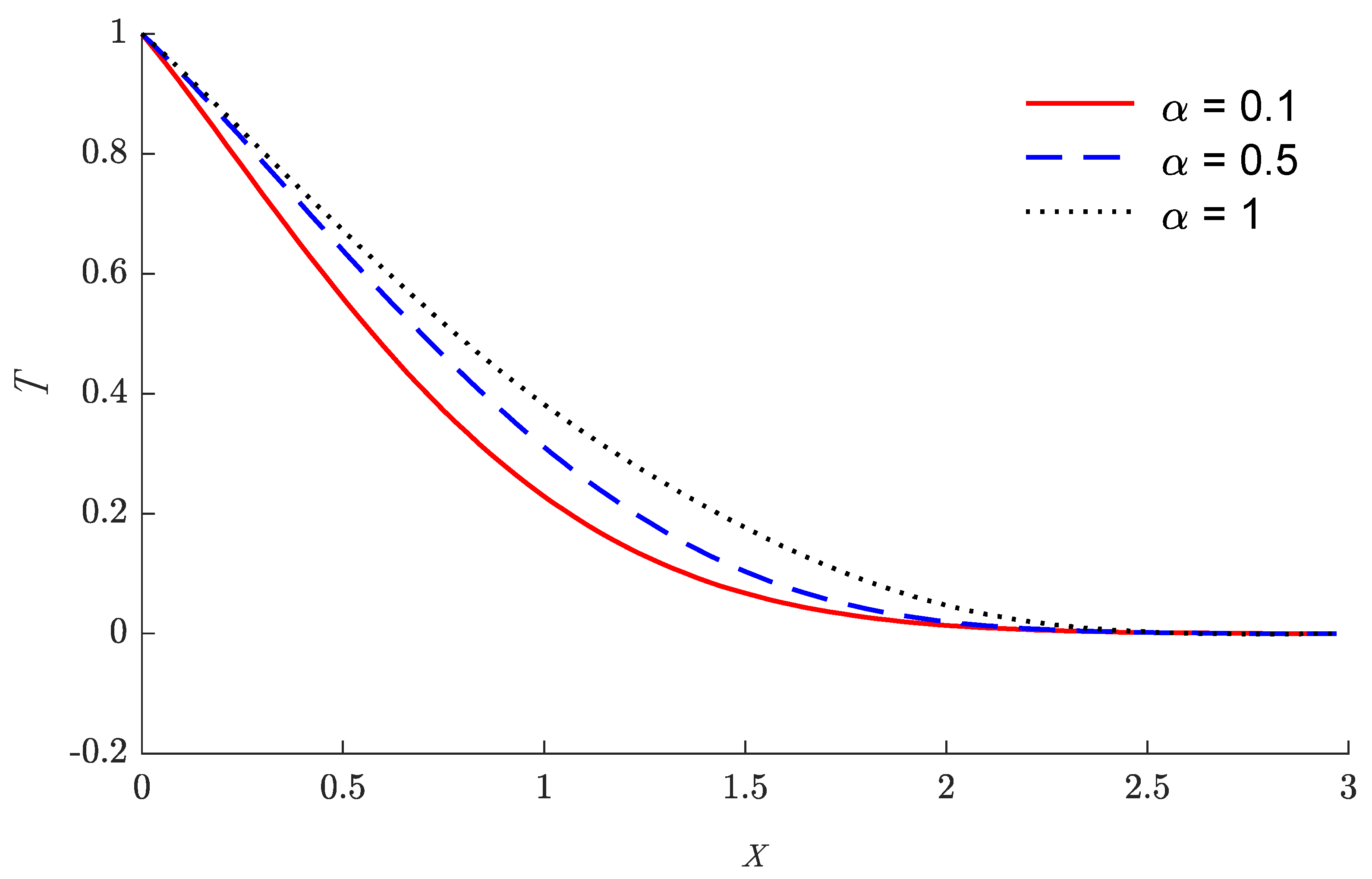
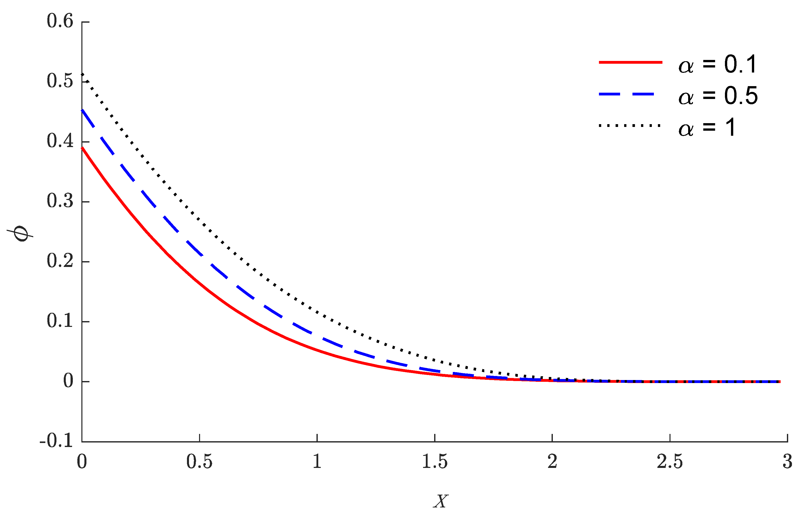
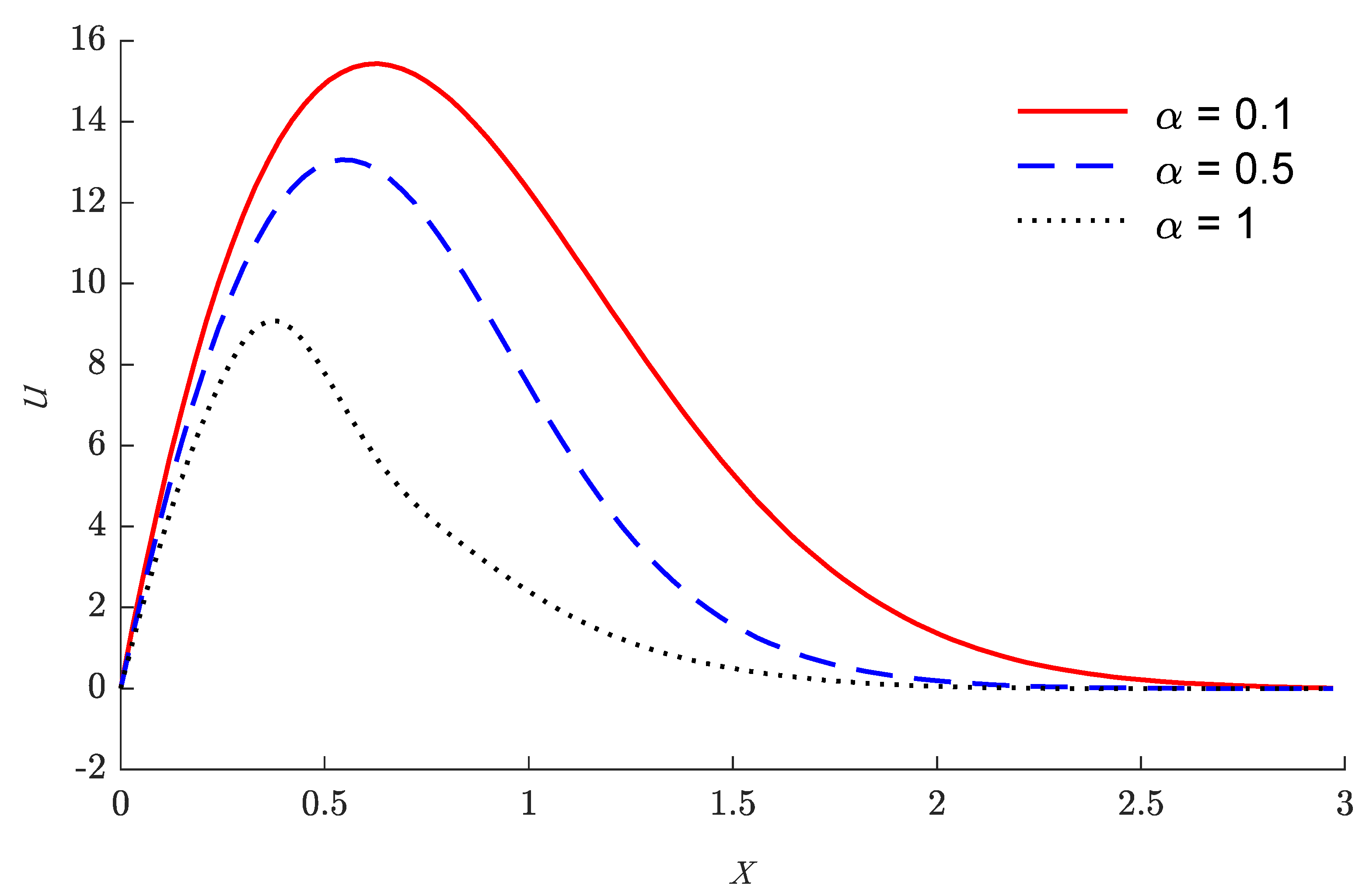
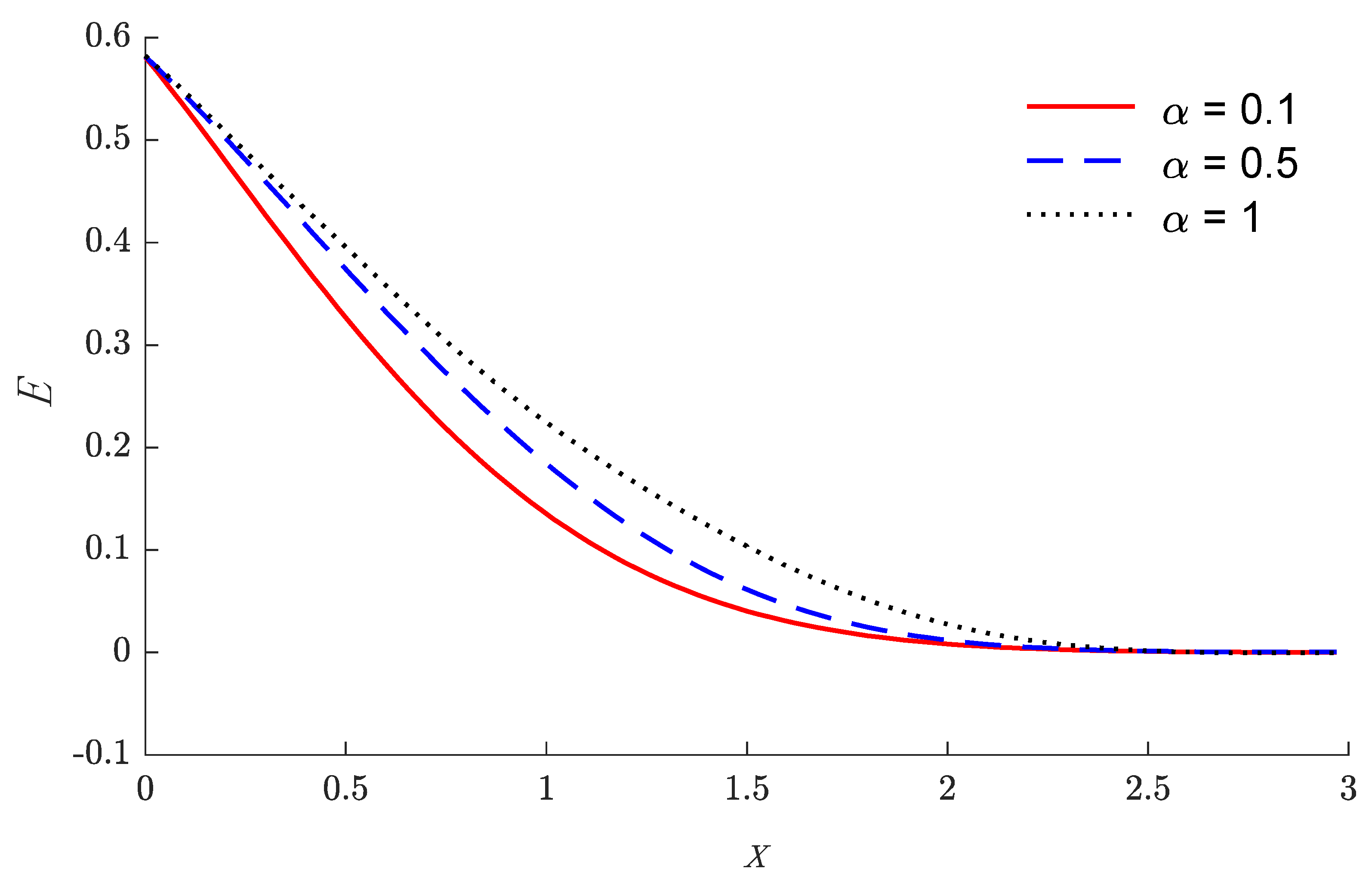
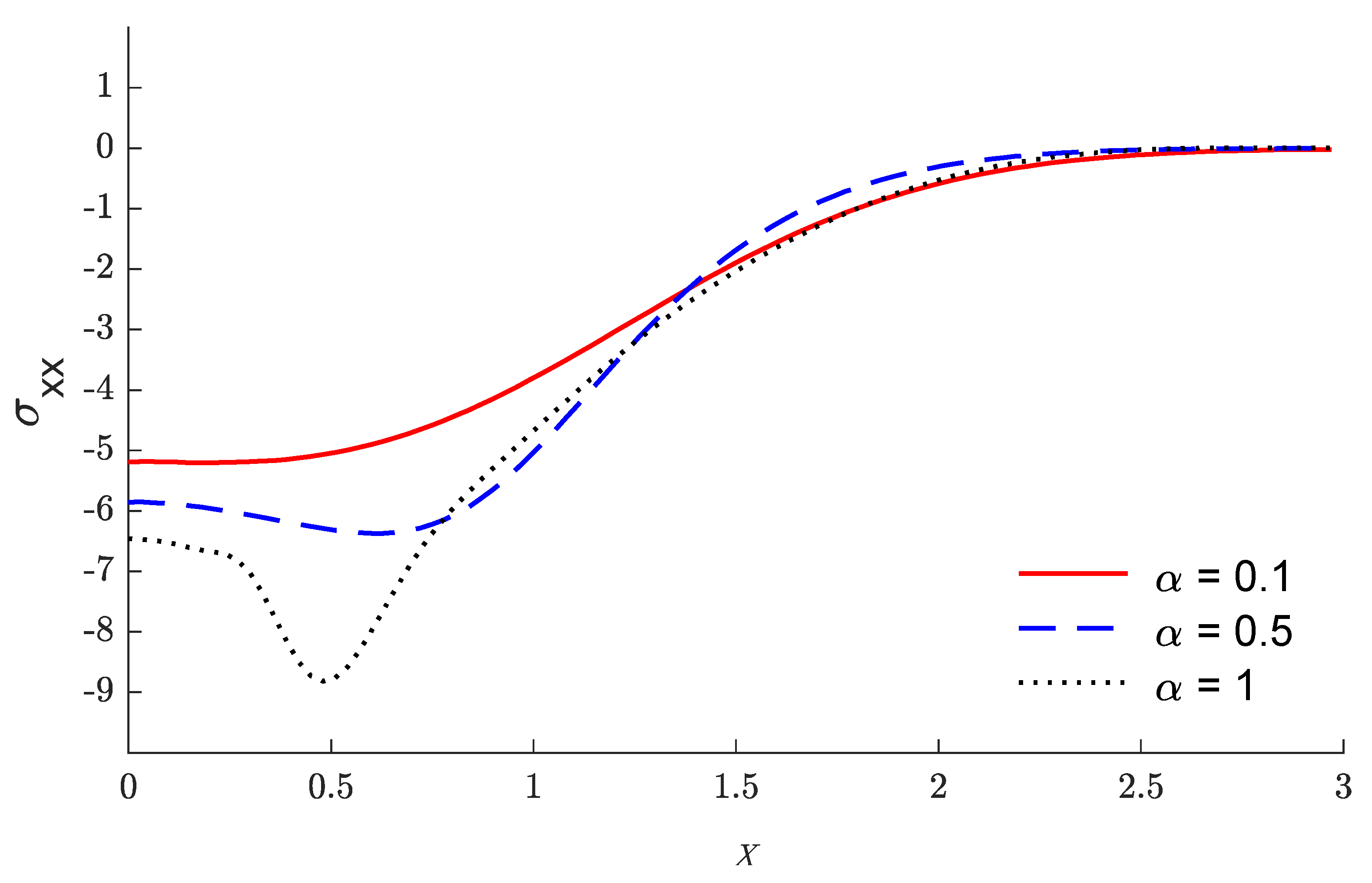
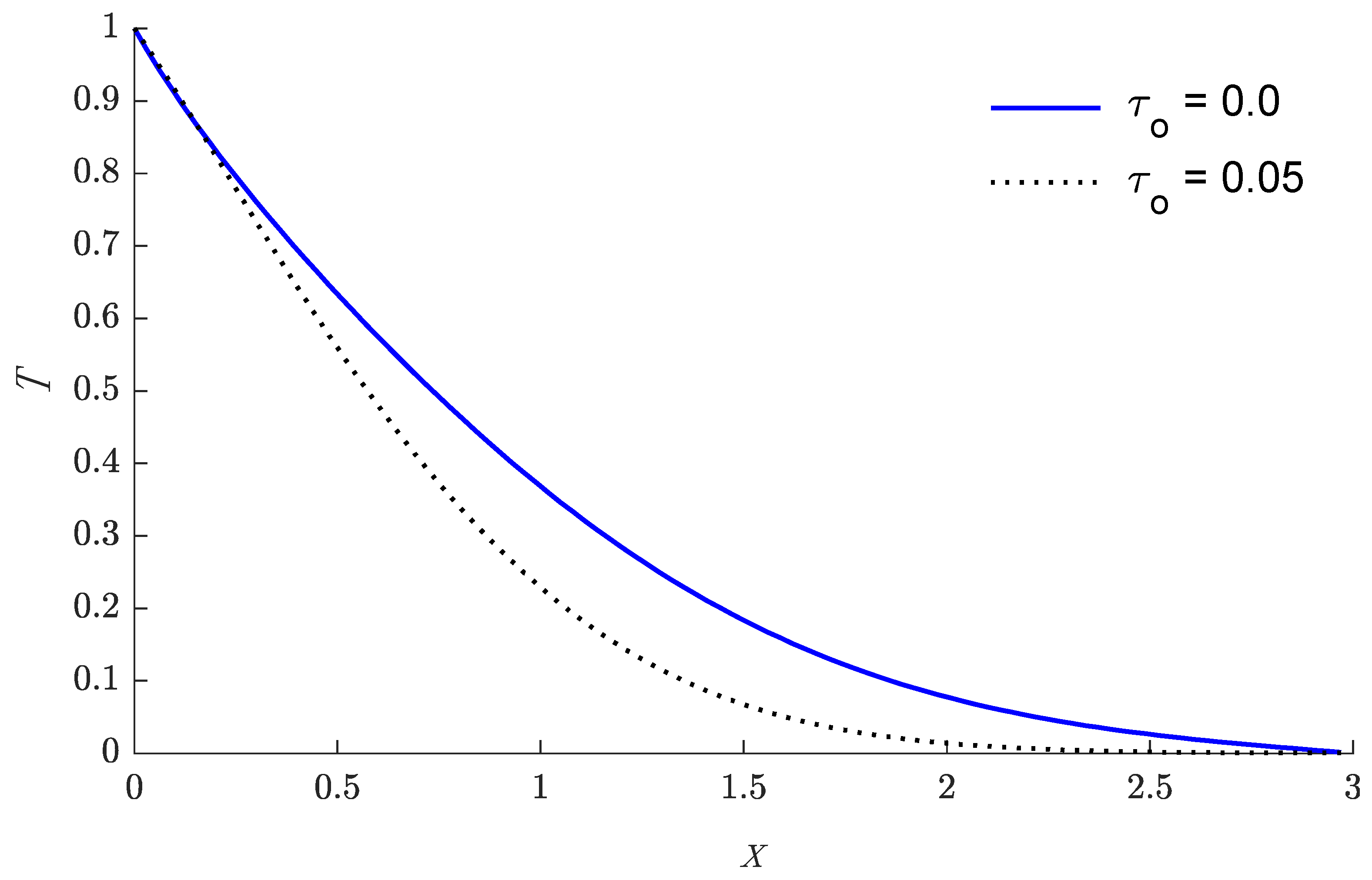
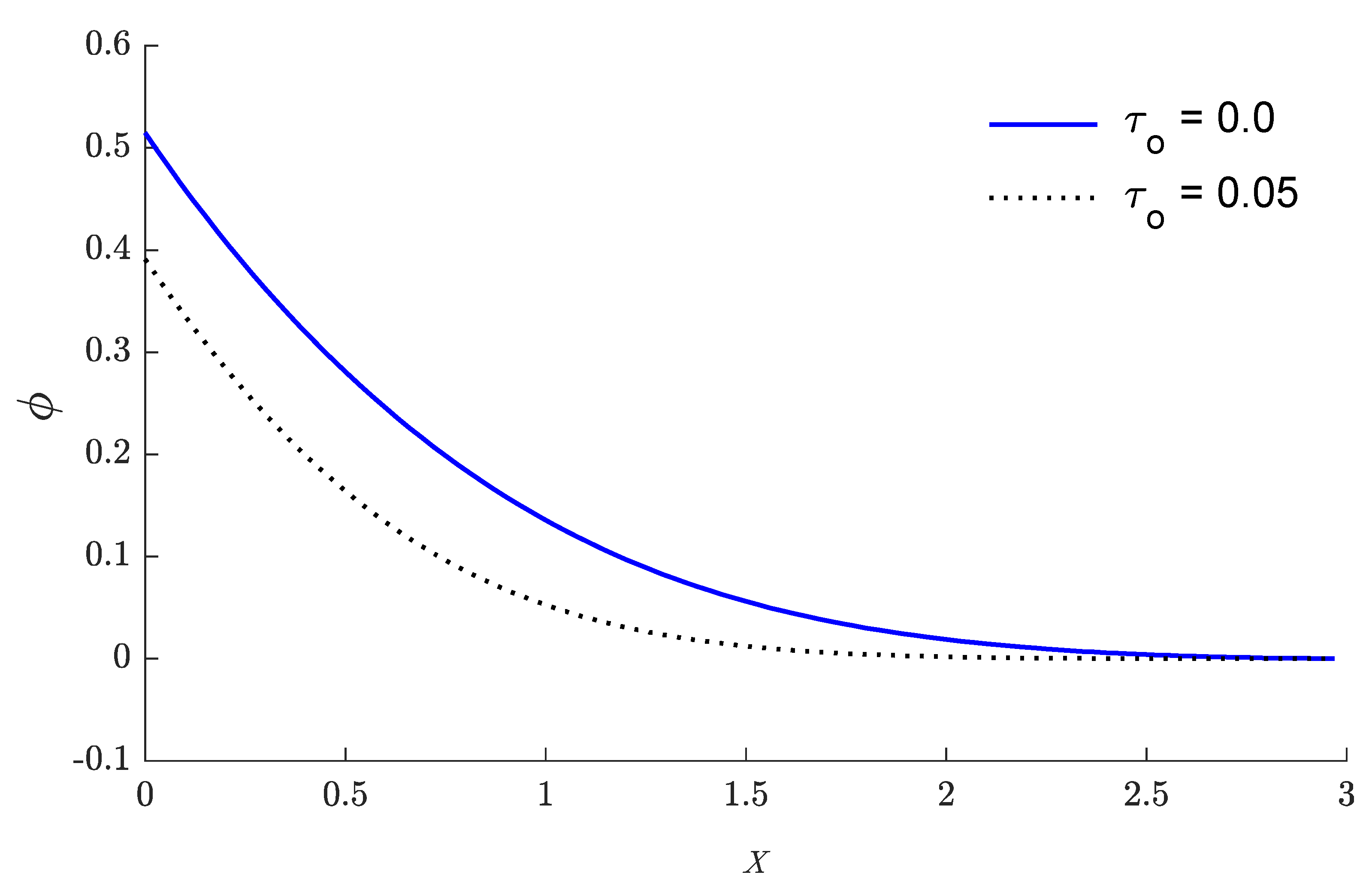
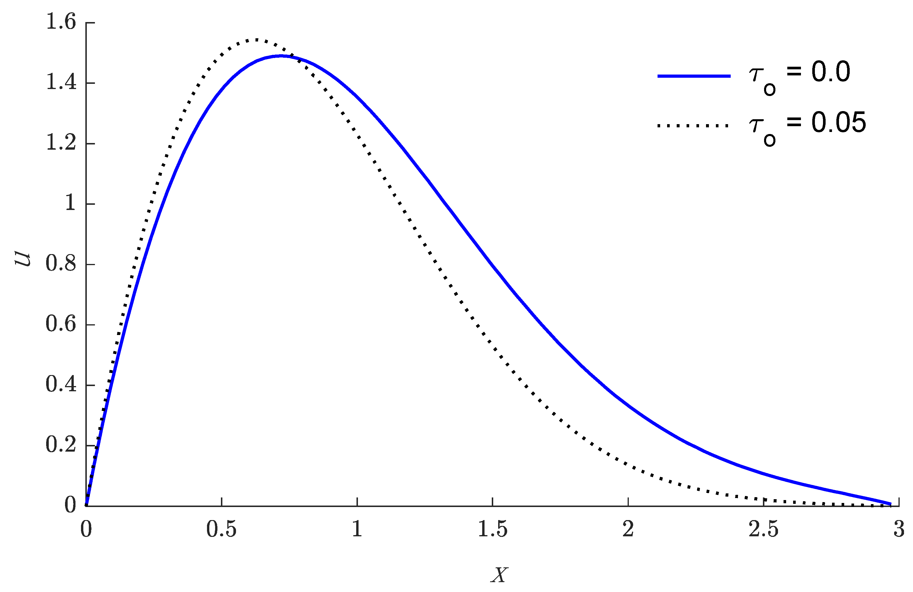
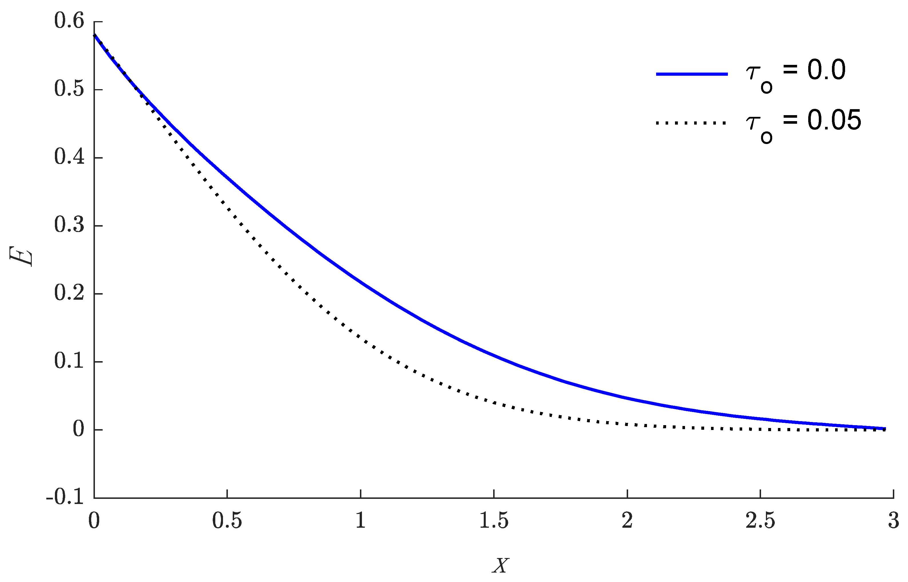
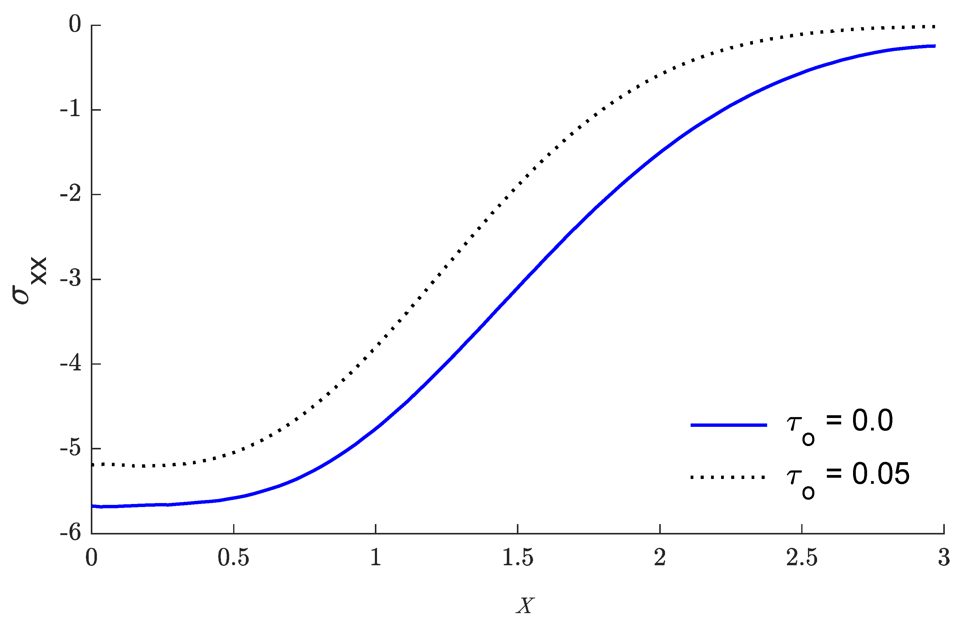
On the basis of the above dataset, in the context of the fractional-order thermoelastic model, the nature of the governing equations, in essence, is characterized by the fractional-order parameter . In the calculations, to study how the fractional-order parameter , as well as the thermal relaxation time, influences the variations of the considered variables, three different values for , (i.e.,) and with and with thermal relaxation time for , (i.e.,) are taken at time . The obtained results are illustrated in Figure 1, Figure 2, Figure 3, Figure 4, Figure 5, Figure 6, Figure 7, Figure 8, Figure 9 and Figure 10. Figure 1, Figure 2, Figure 3, Figure 4 and Figure 5 explain the physical quantities calculated numerically along the distance for three values of fractional-order parameter with thermal relaxation time . Figure 6, Figure 7, Figure 8, Figure 9 and Figure 10 explain the physical quantities calculated numerically along the distance , with and without thermal relaxation time, when the fractional-order parameter . Numerical calculations are carried out for the displacement, the temperature, electric potential, the electric field and the stress variations along the distance in the context of the fractional thermoelastic model with one thermal relaxation time. Figure 1 and Figure 6 demonstrate the variation of temperature along the distance. It is noticed that the temperature of the solid phase begins by its maximum value at and gradually reduces with the increasing of the distanceuntil zeros beyond a wave front for the thermoelastic model satisfies the boundary conditions of the problem. Figure 2 and Figure 7 show the variation of the electric potential as a function of the distance. It is observed that the electric potential has maximum values on and reduces with the rising of the distance to come to zero according to the values of fractional-order parameter and the thermal relaxation time . The variations of displacement through the distance are shown in Figure 3 and Figure 8. It is clear that the displacement begins from zero, which satisfies the boundary conditions of the problem after rising up to maximum values at a specific location within easy reach of the surface. Figure 4 and Figure 9 show the variations of the electric field with respect to the distance . It is clear that it starts from maximum values, after that it decreases with the rising of the distance to come to zero. Figure 5 and Figure 10 show the effects of the of fractional-order parameter and the thermal relaxation time in the stress with respect to the distance. As expected, it clear that the fractional-order parameter and the thermal relaxation time have the great effect on the values of all physical quantities.
Figure 1.
The temperature distributions via the distance for three values of fractional parameter.

When :
Figure 2.
The electric potential distribution via the distance for three values of fractional parameters.
Figure 2.
The electric potential distribution via the distance for three values of fractional parameters.

When :
Figure 3.
The displacement distributions via the distance for three values of fractional parameters.
Figure 3.
The displacement distributions via the distance for three values of fractional parameters.

When :
Figure 4.
The electric field distributions via the distance for three values of fractional parameters.
Figure 4.
The electric field distributions via the distance for three values of fractional parameters.

When :
Figure 5.
The stress distribution via the distance for three values of fractional parameters.

When :
Figure 6.
The temperature distributions via the distance with and without thermal relaxation time.

When :
Figure 7.
The electric potential distribution via the distance with and without thermal relaxation time.
Figure 7.
The electric potential distribution via the distance with and without thermal relaxation time.

When :
Figure 8.
The displacement distribution via the distance with and without thermal relaxation time.

When :
Figure 9.
The electric field distribution via the distance with and without thermal relaxation time.
Figure 9.
The electric field distribution via the distance with and without thermal relaxation time.

When :
Figure 10.
The stress distribution via the distance with and without thermal relaxation time.

When .
7. Conclusions
In this work, the responses of thermoelastic–piezoelectric materials exposed to thermal loading are studied using the model of thermoelasticity with thermal relaxation time. The coupled governing equations of thermoelasticity and piezoelectricity are presented. It is expected that the present finite element method can be applied to generalized piezo-thermo-elastic problems. Based on this, a rigorous hybrid finite element procedure is developed and has been demonstrated as a highly accurate means in dealing with the fractional time derivative in the piezo-thermo-elastic medium. The achievement of this work can be further extended to solve two-dimensional and three-dimensional cases and will be presented in a subsequent report.
Funding
This project was funded by the Deanship of Scientific Research (DSR) at King Abdulaziz University, Jeddah, under grant no. (G: 242-130-1442). The authors, therefore, acknowledge with thanks DSR for technical and financial support.
Informed Consent Statement
Not applicable.
Data Availability Statement
Not applicable.
Conflicts of Interest
The authors declare no conflict of interest.
References
- Biot, M.A. Thermoelasticity and irreversible thermodynamics. J. Appl. Phys. 1956, 27, 240–253. [Google Scholar] [CrossRef]
- Kaminski, W. Hyperbolic heat conduction equation for materials with a nonhomogeneous inner structure. J. Heat Transf. 1990, 112, 555–560. [Google Scholar] [CrossRef]
- Tzou, D.Y. Experimental support for the lagging behavior in heat propagation. J. Thermophys. Heat Transf. 1995, 9, 686–693. [Google Scholar] [CrossRef]
- Lord, H.W.; Shulman, Y. A generalized dynamical theory of thermoelasticity. J. Mech. Phys. Solids 1967, 15, 299–309. [Google Scholar] [CrossRef]
- Green, A.E.; Lindsay, K.A. Thermoelasticity. J. Elast. 1972, 2, 1–7. [Google Scholar] [CrossRef]
- Green, A.E.; Naghdi, P.M. Thermoelasticity without energy dissipation. J. Elast. 1993, 31, 189–208. [Google Scholar] [CrossRef]
- Green, A.; Naghdi, P. A re-examination of the basic postulates of thermomechanics. Proc. R. Soc. Lond. Ser. A Math. Phys. Sci. 1991, 432, 171–194. [Google Scholar]
- Marin, M. A domain of influence theorem for microstretch elastic materials. Nonlinear Anal. Real World Appl. 2010, 11, 3446–3452. [Google Scholar] [CrossRef]
- Marin, M. A partition of energy in thermoelasticity of microstretch bodies. Nonlinear Anal. Real World Appl. 2010, 11, 2436–2447. [Google Scholar] [CrossRef]
- Cheng, N.; Sun, C. Wave propagation in two-layered piezoelectric plates. J. Acoust. Soc. Am. 1975, 57, 632–638. [Google Scholar] [CrossRef]
- He, T.; Cao, L.; Li, S. Dynamic response of a piezoelectric rod with thermal relaxation. J. Sound Vib. 2007, 306, 897–907. [Google Scholar] [CrossRef]
- Akbarzadeh, A.H.; Babaei, M.H.; Chen, Z.T. Thermopiezoelectric analysis of a functionally graded piezoelectric medium. Int. J. Appl. Mech. 2011, 3, 47–68. [Google Scholar] [CrossRef]
- Ma, Y.; He, T. Dynamic response of a generalized piezoelectric-thermoelastic problem under fractional order theory of thermoelasticity. Mech. Adv. Mater. Struct. 2016, 23, 1173–1180. [Google Scholar] [CrossRef]
- Saeed, T.; Abbas, I. Effects of the Nonlocal Thermoelastic Model in a Thermoelastic Nanoscale Material. Mathematics 2022, 10, 284. [Google Scholar] [CrossRef]
- Guha, S.; Singh, A.K. Plane wave reflection/transmission in imperfectly bonded initially stressed rotating piezothermoelastic fiber-reinforced composite half-spaces. Eur. J. Mech. A/Solids 2021, 88, 104242. [Google Scholar] [CrossRef]
- Ragab, M.; Abo-Dahab, S.; Abouelregal, A.E.; Kilany, A. A thermoelastic piezoelectric fixed rod exposed to an axial moving heat source via a dual-phase-lag model. Complexity 2021, 2021, 5547566. [Google Scholar] [CrossRef]
- Biswas, S. Surface waves in piezothermoelastic transversely isotropic layer lying over piezothermoelastic transversely isotropic half-space. Acta Mech. 2021, 232, 373–387. [Google Scholar] [CrossRef]
- Yang, Z.; Sun, L.; Zhang, C.; Zhang, C.; Gao, C. Analysis of a composite piezoelectric semiconductor cylindrical shell under the thermal loading. Mech. Mater. 2022, 164, 104153. [Google Scholar] [CrossRef]
- Singh, S.; Singh, A.; Guha, S. Shear waves in a Piezo-Fiber-Reinforced-Poroelastic composite structure with sandwiched Functionally Graded Buffer Layer: Power Series approach. Eur. J. Mech. A/Solids 2022, 92, 104470. [Google Scholar] [CrossRef]
- Serpilli, M.; Rizzoni, R.; Dumont, S.; Lebon, F. Higher order interface conditions for piezoelectric spherical hollow composites: Asymptotic approach and transfer matrix homogenization method. Compos. Struct. 2022, 279, 114760. [Google Scholar] [CrossRef]
- Abbas, I.A.; Kumar, R. Deformation due to thermal source in micropolar generalized thermoelastic half-space by finite element method. J. Comput. Theor. Nanosci. 2014, 11, 185–190. [Google Scholar] [CrossRef]
- Abbas, I.A.; Kumar, R.; Chawla, V. Response of thermal source in a transversely isotropic thermoelastic half-space with mass diffusion by using a finite element method. Chin. Phys. B 2012, 21, 084601. [Google Scholar] [CrossRef]
- Palani, G.; Abbas, I. Free convection MHD flow with thermal radiation from an impulsively started vertical plate. Nonlinear Anal. Model. Control 2009, 14, 73–84. [Google Scholar] [CrossRef] [Green Version]
- Abbas, I.A.; El-Amin, M.; Salama, A. Effect of thermal dispersion on free convection in a fluid saturated porous medium. Int. J. Heat Fluid Flow 2009, 30, 229–236. [Google Scholar] [CrossRef]
- Abbas, I.A.; Marin, M. Analytical Solutions of a Two-Dimensional Generalized Thermoelastic Diffusions Problem Due to Laser Pulse. Iran. J. Sci. Technol. Trans. Mech. Eng. 2018, 42, 57–71. [Google Scholar] [CrossRef]
- Saeed, T.; Abbas, I.; Marin, M. A GL Model on Thermo-Elastic Interaction in a Poroelastic Material Using Finite Element Method. Symmetry 2020, 12, 488. [Google Scholar] [CrossRef] [Green Version]
- Kumar, R.; Gupta, V.; Abbas, I.A. Plane deformation due to thermal source in fractional order thermoelastic media. J. Comput. Theor. Nanosci. 2013, 10, 2520–2525. [Google Scholar] [CrossRef]
- Hobiny, A.; Abbas, I.A. Analytical solutions of photo-thermo-elastic waves in a non-homogenous semiconducting material. Results Phys. 2018, 10, 385–390. [Google Scholar] [CrossRef]
- Abo-Dahab, S.M.; Abbas, I.A. LS model on thermal shock problem of generalized magneto-thermoelasticity for an infinitely long annular cylinder with variable thermal conductivity. Appl. Math. Model. 2011, 35, 3759–3768. [Google Scholar] [CrossRef]
- Marin, M.; Othman, M.I.A.; Seadawy, A.R.; Carstea, C. A domain of influence in the Moore–Gibson–Thompson theory of dipolar bodies. J. Taibah Univ. Sci. 2020, 14, 653–660. [Google Scholar] [CrossRef]
- Alotaibi, H.; Abo-Dahab, S.; Abdlrahim, H.; Kilany, A. Fractional calculus of thermoelastic p-waves reflection under influence of gravity and electromagnetic fields. Fractals 2020, 28, 2040037. [Google Scholar] [CrossRef]
- Sharma, J.; Walia, V.; Gupta, S. Reflection of piezothermoelastic waves from the charge and stress free boundary of a transversely isotropic half space. Int. J. Eng. Sci. 2008, 46, 131–146. [Google Scholar] [CrossRef]
- Ezzat, M.A. Thermoelectric MHD non-Newtonian fluid with fractional derivative heat transfer. Phys. B Condens. Matter 2010, 405, 4188–4194. [Google Scholar] [CrossRef]
- Ezzat, M.; Ezzat, S. Fractional thermoelasticity applications for porous asphaltic materials. Pet. Sci. 2016, 13, 550–560. [Google Scholar] [CrossRef] [Green Version]
- Mohamed, R.; Abbas, I.A.; Abo-Dahab, S. Finite element analysis of hydromagnetic flow and heat transfer of a heat generation fluid over a surface embedded in a non-Darcian porous medium in the presence of chemical reaction. Commun. Nonlinear Sci. Numer. Simul. 2009, 14, 1385–1395. [Google Scholar] [CrossRef]
- Stehfest, H. Algorithm 368: Numerical inversion of Laplace transforms [D5]. Commun. ACM 1970, 13, 47–49. [Google Scholar] [CrossRef]
Publisher’s Note: MDPI stays neutral with regard to jurisdictional claims in published maps and institutional affiliations. |
© 2022 by the author. Licensee MDPI, Basel, Switzerland. This article is an open access article distributed under the terms and conditions of the Creative Commons Attribution (CC BY) license (https://creativecommons.org/licenses/by/4.0/).
Share and Cite
MDPI and ACS Style
Saeed, T. Hybrid Finite Element Method to Thermo-Elastic Interactions in a Piezo-Thermo-Elastic Medium under a Fractional Time Derivative Model. Mathematics 2022, 10, 650. https://0-doi-org.brum.beds.ac.uk/10.3390/math10040650
AMA Style
Saeed T. Hybrid Finite Element Method to Thermo-Elastic Interactions in a Piezo-Thermo-Elastic Medium under a Fractional Time Derivative Model. Mathematics. 2022; 10(4):650. https://0-doi-org.brum.beds.ac.uk/10.3390/math10040650
Chicago/Turabian StyleSaeed, Tareq. 2022. "Hybrid Finite Element Method to Thermo-Elastic Interactions in a Piezo-Thermo-Elastic Medium under a Fractional Time Derivative Model" Mathematics 10, no. 4: 650. https://0-doi-org.brum.beds.ac.uk/10.3390/math10040650
Note that from the first issue of 2016, this journal uses article numbers instead of page numbers. See further details here.