Single-Image Super-Resolution Neural Network via Hybrid Multi-Scale Features

Abstract

In this paper, we propose an end-to-end single-image super-resolution neural network by leveraging hybrid multi-scale features of images. Different from most existing convolutional neural network (CNN) based solutions, our proposed network depends on the observation that image features extracted by CNN contain hybrid multi-scale features: both multi-scale local texture features and global structural features. By effectively exploiting these multi-scale and local-global features, our network involves far fewer parameters, leading to a large decrease in memory usage and computation during inference. Our network benefits from three key modules: (1) an efficient and lightweight feature extraction module (EFblock); (2) a hybrid multi-scale feature enhancement module (HMblock); and (3) a reconstruction–restoration module (DRblock). Experiments on five popular benchmarks demonstrate that our super-resolution approach achieves better performance with fewer parameters and less memory consumption, compared to more than 20 SOTAs. In summary, we propose a novel multi-scale super-resolution neural network (HMSF), which is more lightweight, has fewer parameters, and requires less execution time, but has better performance than the state-of-the-art methods. Compared to SOTAs, this method is more practical and better suited to run on constrained devices, such as PCs and mobile devices, without the need for a high-performance server.

1. Introduction

Single-image super-resolution (SISR) seeks to reconstruct a high-resolution image with the high-frequency information (meaning the details) restored from its low-resolution counterpart [1]. SISR offers many practical applications, such as video monitoring, remote sensing, video coding and medical imaging. On the one hand, SISR reduces the cost of obtaining high-resolution images, allowing researchers to acquire HR images, using personal computers instead of sophisticated and expensive optical imaging equipment. On the one hand, SISR reduces the cost of obtaining high-resolution images, allowing researchers to acquire HR images, using personal computers instead of sophisticated and expensive optical imaging equipment. On the other hand, SISR reduces the cost of information transmission, i.e., high-resolution images can be obtained by decoding the transmitted low-resolution image information using SISR. Many efforts have been made to deal with such a challenging yet ill-posed problem, due to the unknown high-resolution version of a low-resolution image.

Many traditional methods [2,3,4] have been proposed to obtain high resolution (HR) images from their low resolution (LR) versions by establishing a mapping relationship between LR images and HR images. These methods are fast, lightweight and effective, which make them preferable as basic tools in SISR tasks [5]. However, there is a shared and inherent problem in applying them: the tedious parameter adjustment. Obtaining desired results relies on continually tweaking parameters to accommodate various inputs. This inconvenience has an adverse impact on both efficiency and the user experience.

In recent years, there have been considerable efforts made with convolutional neural networks—CNN-based SISR methods—by EDSR [6], DRRN [7], LapSRN [8], MemNet [9], CARN [10], IDN [11], MADNet [12], MRFN [13], and DRFN [14]. Such pioneering methods [15,16], despite having made use of only a few convolution layers, have validated that CNN exhibits better performance than do many traditional SISR methods. Subsequent efforts have focused mainly on improving the network structure by increasing its depth and width. Doing so can result in better performance with more trainable parameters to establish a more stable mapping relationship between LR and HR images. Extensive studies (e.g., [17]) with very deep neural networks [13] have shown that a deeper network [18] will have better performance than a shallower one [15,16]. However, there are many parameters to optimize for deep neural networks; furthermore, the training process consumes massive amounts of data to avoid overfitting. A common drawback is that such efforts have considered only the deepening of the network, while not sufficiently leveraging various extracted features.

Reducing the number of both the parameters and calculations is important in actual application scenarios. For example, it would be difficult to execute a model on mobile devices if the model were to require so much memory; also, it would provide an unfriendly user experience, due to the slow execution speed. To achieve better performance via a lightweight model, we define the hybrid multi-scale features in SISR as local multi-scale features and global multi-scale features, containing the thickness of texture features and structural features from detail to structure. We use the feature map obtained by interpolation as the basic frame of SISR. After the extraction of features by the efficient lightweight residual feature extraction module, the local multi-scale and global multi-scale enhancement modules and reconstruction modules are enhanced and fused, and the Charbonnier loss function is used for training. Finally, the mapping relationship between the LR and HR images is established, and the result is the SR image. We focus on fewer parameters to obtain good enhancement effects. Unlike other networks that only use convolutional layers to extract features, ours makes use of an efficient and lightweight feature extraction module, EFblock, to extract features from LR images, then inputs the features into the hybrid multi-scale enhancement module HMblock, which includes the local multi-scale feature extraction module called RF as well as a global feature enhancement module. After the hybrid multi-scale features are extracted and enhanced, through the reconstruction and fusion module DRBlock, the features are restored to the up-sampled LR image to obtain the SR image. In terms of mixed multi-scale features, the deeper convolutional neural network module is sufficient to extract the structural features of the image, while the shallower convolutional neural network module can extract the texture features of the image. The residual connection can compensate for feature extraction loss of the global characteristics in the process. In terms of local multi-scale features, different receptive field sizes of the convolution kernel can extract texture features of different thicknesses. Therefore, we study the dependence and complementation solution between the depth and the size of the convolution kernel receiving field between the structural features and the texture features. In summary, the main contributions of this article are as follows:

• We propose a novel efficient and lightweight feature extraction module, called EFblock. It uses both grouped convolution and point convolution, and introduces both a global and local residual connection to improve the integrity of the feature extraction. Although EFblock has fewer parameters and less computation, it exhibits better performance than existing CNN-based methods.
• We formulate the concept of hybrid multi-scale features, qualitatively dividing multi-scale features into local multi-scale and global multi-scale features; unlike other other multi-scale based solutions, ours uses only shallow local multi-scale features. This shallow local multi-scale extraction block mainly extracts texture features, while the deep convolutional layer extracts skeleton and structural features; together, they constitute hybrid multi-scale features.
• Existing multi-scale based methods have a large number of parameters and are not flexible enough. They only focus on regular receptive areas and cannot fully extract multi-scale information. To solve this problem, we propose a bottleneck stack structure RF to extract the local multi-scale texture feature. Different from other schemes that only use different sizes of convolution kernels [19] or stacked 3 × 3 convolution kernels [13], we flexibly utilize a dilated convolution [20], and also obtain different sizes of receptive fields by controlling the dilation rate, as well as adding deformable convolution [21] to further yield irregular receptive areas. Because of the use of the bottleneck structure, the RF module not only yields multi-scale receptive fields, but also greatly reduces the number of parameters and the burden of calculation.

2. Related Works

In the early days, the task of SISR was defined as a mathematical mapping problem [2,3,4]. Some of them used regression to restore the image [4], some of them used random forest to tackle the problem [2], and some of them [22] used decision-making theory [23,24] to restore the LR images. Recently, deep learning was successful in many computer vision tasks, including SISR. Based on the needs of practical applications, lightweight models are currently the focus of attention. Here, we will summarize the SISR methods based on deep learning, while focusing on lightweight SISR methods.

2.1. Deep CNN-Based SISR

Like other computer vision tasks, SISR has made significant progress through deep convolutional neural networks. Dong et al. first proposed SRCNN [15] based on shallow CNNs. That method involves up-samples of images through bicubic interpolation. With three convolutional layers—as well as patch extraction and representation, plus nonlinear mapping and image reconstruction—the network was established. Later, that team proposed FSRCNN [16], while Shi et al. proposed ESPCN [25]. Meanwhile, Lai et al. proposed a Laplacian pyramid super-resolution network [8], which takes low-resolution images as input and gradually reconstructs the sub-band residuals of high-resolution images. Tai et al. used a persistent memory network (MemNet) [9] by using a very deep network. Tian et al. proposed a coarse-to-fine CNN method [26] that, from the perspective of low-frequency features and high-frequency features, adds heterogeneous convolutions and refinement blocks to extract and process high-frequency and low-frequency features separately. Wei et al. [27] used cascading dense connections to extract features of different fineness from different depth convolutional layers. Jin et al. adopted a framework [28] to flexibly adjust the architecture of the network, adapting different kinds of images. DRCN [29] used a deeply recursive convolutional network to improve performance without introducing new parameters for additional convolutions. DRRN [7] improved DRCN by using residual networks. Lim et al. proposed an enhanced deep residual network (EDSR) [6]. Liu et al. [30] proposed an improved version of U-Net based on a multi-level wavelet. Li et al. [31] proposed exploiting self-attention and facial semantics to obtain a super-resolution face image. Most studies of SISR achieved better performance by deepening the network or by adding the residual connection. However, deep depths make these methods difficult to train, while more parameters not only cause excessive memory consumption during inference, but also slow down the execution speed. Therefore, we introduce a lightweight and efficient SISR model.

In terms of lightweight models, Hui et al. proposed IDN [11] by knowledge distillation to distill and extract features of each layer of the network and learn the complementary relationship among them to reduce parameters. CARN [10] used a lightweight cascaded residual network; the local and global levels use cascading mechanisms to integrate features from different scale layers in order to receive more information. However, that method still involves 1.5 M parameters, and consumes too much memory. Ahn et al. [32] proposed a lightweight residual network that uses grouped convolution to reduce the number of parameters, as well as weight classification to enhance the effect of super-resolution. Yao et al. proposed GLADSR [33] with dense connections. Tian et al. proposed LESRCNN [34], using dense cross-layer connections and advanced sub-pixel convolution to reconstruct images. Lan et al. proposed MADNet [12], which contains many kinds of networks. He et al. [13] introduced a multi-scale residual network.

Existing lightweight SISR methods can compress the number of parameters and calculations, but doing so results in loss of performance. In contrast, our method can achieve better super-resolution performance despite a small number of parameters and reduced memory consumption.

2.2. Lightweight Neural Networks

Many recent super-resolution methods have focused on the lightweight nature of neural networks. We also focus on these features. Many lightweight network structures have been proposed, including dense networks [10,34], which use dense connections or residual connections to fully reuse functions. These methods are an efficient improvement for deep neural networks, but are inadequate for lightweight networks. Therefore, we need to pay more attention to efficient lightweight network skeletons. In subsequent works, researchers have proposed several derivative versions, with the introduction of cross-layer connections within the network, reusing functions to achieve better performance. Iandola et al. proposed SqueezeNet [35], using a squeeze layer and a convolution layer with a kernel size of 1 × 1 to convolve the feature map of the previous layer, thereby reducing the dimensionality of the feature map. Shufflenet V1 [36] and V2 [37] flexibly used pointwise grouped convolution and channel shuffle to achieve efficient classification effects on ImageNet [38]. MobileNet [39] constructed an effective network by applying—in a subsequent version—the deep separable convolution introduced by Sifre et al. MobileNet-V2 [40] also made use of methods, such as grouped convolution and point convolution, and introduced an attention mechanism. The design of the MobileNet-V3 [41] network utilized the NAS (network architecture search [42]) algorithm to search for a very efficient network structure. In contrast, the EFblock that we propose uses global and local residual connections, deep separable convolution, grouped convolution and point convolution. Our method comprehensively considers the needs of light weight and super-resolution, and extracts features efficiently with a small number of parameters.

2.3. Multi-Scale Feature Extraction

Multi-scale feature extraction is widely used in computer vision tasks, such as in semantic segmentation, image restoration and image super-resolution. The most basic feature is that filters with different convolution kernel sizes can extract features of different fineness. Szegedy et al. proposed a multi-scale module [19] called the Inception module. It uses convolution filters with different convolution kernel sizes to extract features in parallel, enabling the network to obtain different sizes of receptive fields, then extracting different characteristics of fineness. In a subsequent version, the authors processed batch normalization in Inception-V2 [43], which accelerates the training of the network. In Inception-V3 [44], the authors added a new optimizer and asymmetric convolution. Recently, the application of multi-scale convolutional layers was widely demonstrated in tasks such as deblurring and denoising. He et al. [13] introduced a multi-scale residual network with image features to significantly improve the performance of the image super-resolution. However, these methods focus only on local multi-scale features, ignoring the concept of a global scale. There is room for further improvement to realize the multi-scale network structure. As discussed above, we propose a hybrid multi-scale that, broadly, can be defined as local multi-scale and global multi-scale: the “local multi-scale” refers to the texture feature, and the “global multi-scale” refers to the structure feature. We experimented with this idea; the specific experimental details are introduced later.

3. Methodology

We propose a hybrid multi-scale feature neural network (HMSF). In this section, we first introduce the overall structure of HMSF and analyze the detailed information of each component. Next, we focus on analyzing our hybrid multi-scale enhancement module, HMblock.

3.1. Network Structure

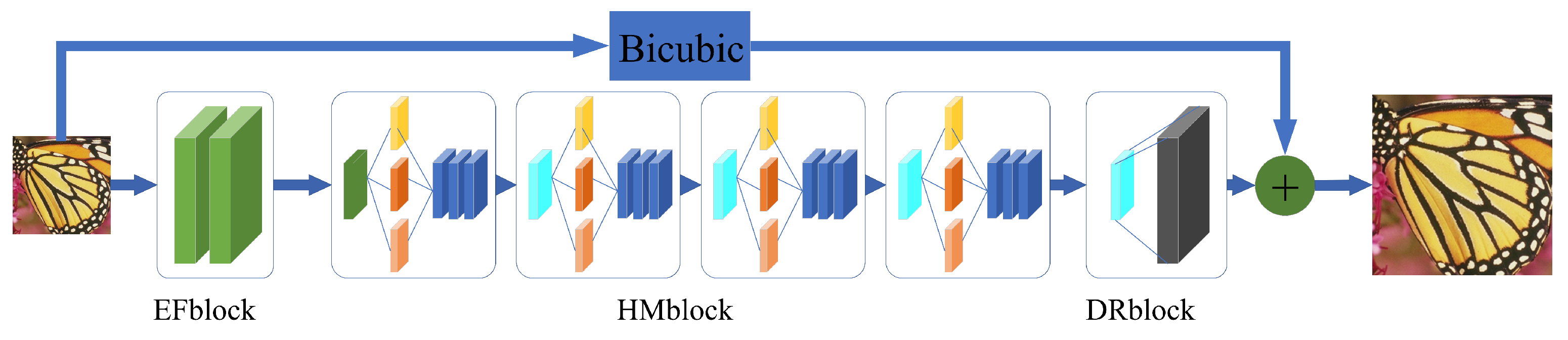
The proposed method consists of three main parts (see Figure 1): an efficient feature extraction module, EFblock; a global and local multi-scale enhancement module, HMblock; and an image reconstruction module, DRBlock.

3.1.1. EFblock

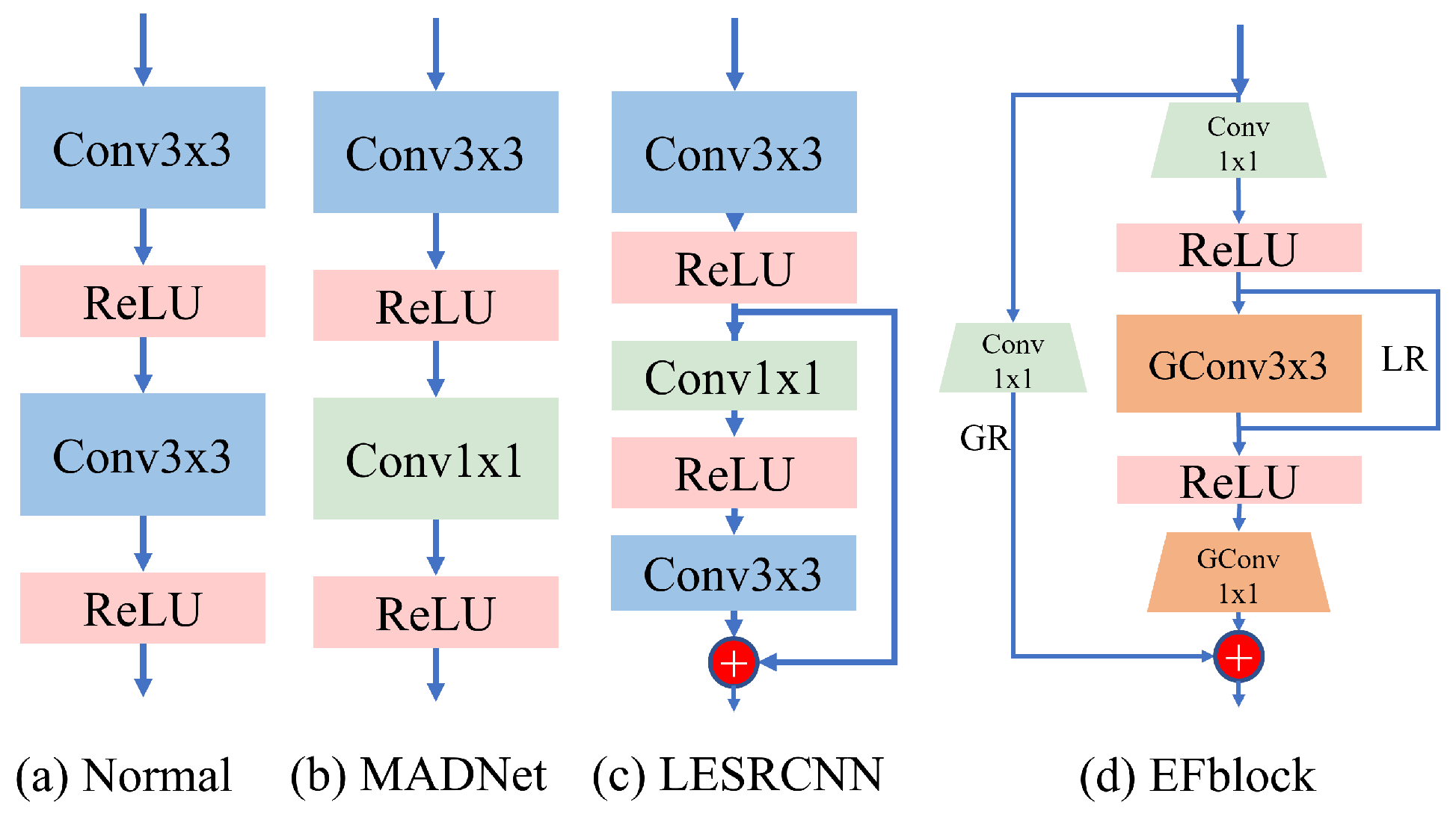
As shown in Figure 2, many lightweight super-resolution methods use either a scale of 3 × 3 convolutional layers or 1 × 1 convolutional layers to extract features. We believe that the features extracted in this way are inefficient because adding a 3 × 3 convolutional layer increases many parameters. In light of that dilemma, and inspired by other efficient networks [35,36,41], we designed a lightweight and efficient feature extraction module, EFblock. Its performance is stronger than the standard convolution, and its parameters and calculations are relatively small. We first use a point convolution layer to upgrade the original image to the size that needs to be processed, then use grouped convolution, where, to extract features, the input size is equal to the output size. Finally, grouped point convolution is used to promote the feature to the dimension of the output. This combination of grouped convolution and point convolution can effectively reduce parameters and calculations.

As shown in

Table 1. Comparing EFblock and standard convolution layers from parameter and calculation number, and number of activation functions.

Method	Layer	Dimension	Total Param. Total Madd	Activation
Conv3 × 3 block	Conv1	3-32	19 K	2
	Conv2	32-64	4.4 G
EFblock	Block1	3-32-64	16 K	6
	Block2	64-64-64	3.7 G

, our proposed EFblock is compared with the standard convolutional module. If we use the standard 3 × 3 convolution, there are about 19,000 parameters. If we use EFblock, the number of parameters is reduced to about 16,000. In terms of the number of calculations, we use multi-adds as the evaluation standard; the standard convolution module is 4.4 G, and EFblock is 3.7 G, thereby reducing the number of both parameters and calculations. With the dimensional changes, we find that EFblock has more activation functions, making feature extraction more nonlinear and stronger in characterization. We next consider the global residual connection and the local residual connection. We believe that, in the process of extracting image features, global information will be lost. Therefore, we use global residual connection to compensate for the loss of information, and use point convolution to match the input dimension with the compensation dimension. Between the grouped convolution, we add a local residual connection to compensate for the lack of feature correlation between channels caused by too many groups.

The overall expression of EFblock is as follows. $F_i$ is the feature output by the i-th layer module; PGconv represents the grouped point convolution; Pconv represents the point convolution; and Gconv represents the grouped convolution. GR and LR represent global and local residual connections, respectively.

$$F_i=\mathit{PGConv}\left[\mathit{Gconv}\left[\mathit{PConv}\left[F_{i-1}\right]\right]+\mathit{LR}\right]+\mathit{GR}$$

(1)

If the two residuals cannot be directly connected to the required dimension, point convolution is needed to increase or decrease the dimension:

$$\mathit{LR}=\mathit{PConv}\left[F_{i-1}\right]\left(C_{out}={C_{in}}_{\mathrm{Gconv}}\right)$$

(2)

$$\mathit{GR}=\mathit{PConv}\left[F_{i-1}\right]\left(C_{out}={C_{out}}_{\mathrm{Gconv}}\right)$$

(3)

3.1.2. HMblock

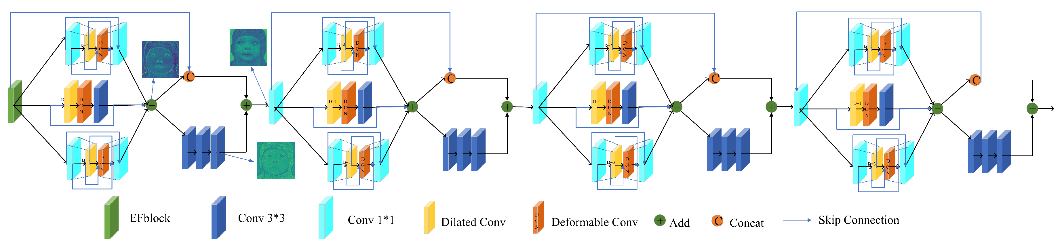
HMblock is the core part of the method. In this module, we define global and local multi-scale features: local texture features and global structural features. As shown in Figure 3, HMblock is divided into shallow multi-scale texture feature extraction blocks as well as deep structure feature extraction blocks. When the number of convolutional layers is shallow, the feature information extracted by the network is rich, and will include the internal texture and external contour of the object in the picture. As the number of convolutional layers becomes deeper and deeper, the network will ignore some detailed textures, saving only the important skeletons in the picture. Of course, the texture feature also contains some structural information, but the information is too rich, and the texture and structure are messy and difficult to distinguish.

The role of HMblock is to merge together texture features that already contain various information with the original structural features, so that the reconstructed SR image possesses an accurate structure and rich texture features. When extracting texture features, we consider multi-scale texture features. Usually, we use convolutional layers with different convolution kernel sizes. The inception [19] module uses 3 × 3, 5 × 5, and 7 × 7 convolutional layers to achieve multi-scale features. Instead of using convolutional layers with different convolution kernel sizes, we construct a bottleneck structure, and use dilated convolution to obtain different sizes of the receptive fields. If we use standard discrete convolutional layers, with ⊗ as the operator of convolution, and defining a discrete function $\mathit{O}ϵ{\mathbb{Z}}^2$ and a discrete convolution kernel $\mathit{P}ϵ{\mathbb{Z}}^2$, the expression can be given as

$$(O\otimes P)\left(i\right)=\sum _{s+t=i}O\left(s\right)P\left(t\right)$$

(4)

When using a standard convolutional layer, the size of the receptive field depends on the size of the convolution kernel. Some methods such as MRFN [13], which uses repeated stacking of 3 × 3 convolutional layers to obtain a large receptive field, will lead to a large increase in the number of parameters and calculations. To minimize that problem, we use dilated convolution and a control dilation factor r to control the size of the receptive field. The operation of dilated convolution can be stated as

$$\left(O{\otimes }_{r}P\right)\left(i\right)=\sum _{s+rt=i}O\left(s\right)P\left(t\right)$$

(5)

The dilated convolution [20] operator of dilation r can be referred to as ${\otimes }_r$. Figure 4 shows that, by using dilation factors of 1 and 2 and 3, we can obtain the receptive fields of 3 × 3, 5 × 5 and 7 × 7.

The features of scenes and objects in natural images are often irregular. In the RF module, even though multi-scale receptive fields have been obtained, the ability to learn irregular features remains inadequate.

For the model to further learn irregular features, we use deformable convolution [21] with offset:

$$\left(O{\otimes }_{d}P\right)\left(i\right)=\sum _{s+t+\mathsf{\Delta }{x}_n=i}O\left(s\right)P\left(t\right)$$

(6)

$\mathsf{\Delta }{x}_n$ is a learnable offset, and should be processed by bilinear interpolation to match the features. We flexibly use residual connection to avoid the checkerboard effect, and compensate for the information lost due to the enlargement of the receptive field. Before and after the RF module, we have added a global residual connection; furthermore, in the middle layer of RF5 and RF7, we have added two local residual connections.

Table 2. Comparing different local multi-scale implementation methods.

Method	RF	Parameter	Madd	Receptive Field
HMblock-${}_{\mathit{inc}}$ [19]	Different conv kernel sizes	0.865 M	138 G	3, 5, 7
HMblock-${}_{\mathit{mrf}}$ [13]	Only stack 3 × 3 conv	0.747 M	111 G	3, 5, 7
HMblock	Bottleneck + Dilated + Deformable	0.523 M	59 G	[3, 5, 7] × Deformable

shows that the number of parameters of the multi-scale method is greatly reduced, compared to Inception style [19] and MRFN style [13].

In the super-resolution task, the structural similarity between the SR image and the HR image is very important, since problems such as distortion and deformation often crop up during processing. After obtaining multi-scale texture features, we consider structural features. Many existing methods [13] quit increasing the depth of this module after extracting the multi-scale texture features. However, doing so is not enough; although texture features contain structural features, the amount of information remains too large—with a gap between texture details and structural details. Without an obvious boundary, the contour of the reconstructed image remains blurred and too smooth. Our idea is to use a deeper convolutional layer to extract the structural features contained in the multi-scale texture features, and merge them again to strengthen the structure outline and fix the texture details to an accurate position.

As shown in Figure 3, we input the features into three multi-scale blocks RF, and connect them with the residual to compensate for the loss of global information:

$$F_{[i,\mathit{T}]}=\sum _{r=3,5,7}(R{F}_r\left[F_{[i-1]}\right]+Re{s}_r)$$

(7)

After obtaining the local multi-scale texture features, we further extract the corresponding structural features through three deeper convolutional layers. We use the local residual connection to register the texture features to the corresponding positions of the structural features. We do not directly add the texture and structural features; instead, we first add a global residual connection link to the texture feature, then use concat to stack the texture feature and the global residual feature, finally adding the structural feature:

$$F_i=F_{[i,\mathit{S}]}+\mathit{Concat}\left[F_{[i,\mathit{T}]},F_{i-1}\right]$$

(8)

Finally, we use a point convolutional layer to fuse the texture features and structural features. Table 2 shows the characteristics of our HMblock compared to other super-resolution core modules. We have used a variety of methods to reduce the number of parameters and made improvements in terms of hybrid multi-scale features.

Table 3. Comparison of different image enhancement blocks: “LMS” means “local multi-scale”, “GMS” means “global multi-scale”, and “HMS” means “hybrid multi-scale”.

Block	LMS	GMS	HMS
CARN	×	×	×
MRF (MRFN)	√	×	×
LESRCNN	×	×	×
HMblock (Ours)	√	√	√

shows the differences between HMSF and other methods used for multi-scale feature extraction.

3.1.3. DRblock

The last module is DRBlock. This module includes a 1 × 1 convolution for dimensionality reduction integration, as well as a PixelShuffle [25] layer for upsampling. DRBlock inputs an H × W low-resolution input image, and through a sub-pixel operation turns it into a high-resolution image of $rH$ × $rW$. However, the realization process is not achieved by directly generating the high-resolution image through interpolation; instead, the process yields $r^2$, the dimensional feature map, through convolution. Then the high-resolution image is obtained through periodic shuffling, where r is the upsampling factor, which is the magnification of the image. The 1 × 1 convolution we used before yields the feature map to be sampled with matching dimensions. After upsampling, we add together the feature map that meets the resolution with the low-resolution enlarged image obtained by bicubic linear interpolation to obtain the super-resolution image.

3.2. Loss Function

We considered using two loss functions to evaluate the difference between the true-value HR and the model-predicted-and-reconstructed SR image. The first loss function is $L2$, which is the mean-squared error (MSE), expressed as follows:

$${\mathcal{L}}_{\mathrm{MSE}}(\widehat{I},I)=\frac{1}{\mathrm{hwc}\sum {\left({\widehat{I}}_{i,j,k}-I_{i,j,k}\right)}^2}$$

(9)

However, the L2 loss function is difficult to use under the influence of noise; its correlation with human visual perception is insufficient, and the potential multi-modal distribution from low-resolution LR to high-resolution HR is not to be found. Oftentimes, the reconstructed image is too smooth. Unlike L2, the L1 loss function is widely used in many super-resolution tasks; many experiments have shown that it improves the effect of super-resolution. Therefore, we have considered using the Charbonnier loss function, which is an improved form of the L1 loss function [8]. To prevent over-fitting, it adds a regular term $\epsilon$ with $1\times {10}^{-3}$ at the end:

$${\mathcal{L}}_{\mathrm{Charbonnier}}(\widehat{I},I)=\frac{1}{\mathrm{hwc}}\sum _{i,j,k}\sqrt{{\left({\widehat{I}}_{i,j,k}-I_{i,j,k}\right)}^2+{ϵ}^2}$$

(10)

We have used the L2 and Charbonnier loss functions to train our model. Experimental results show that the Charbonnier loss function can achieve better training results.

4. Experiments

4.1. Datasets

4.1.1. Training Datasets

In line with state-of-the-art methods [6,10,12,34,45,46,47], we utilized the DIV2K dataset [48] to train our image super-resolution network. DIV2K is a high-quality image dataset, containing 800 training images, 100 testing images and 100 validation images.

4.1.2. Testing Datasets

In keeping with most existing methods, we also evaluated the effectiveness of the developed network on the following benchmark datasets: Set5 [49], Set14 [50], BSD100 [51], Urban100 [52] and Manga109 [53]. Among these datasets, BSD100, Set5, and Set14 consist of images with natural scenes; Urban100 contains urban scenes; and Manga109 consists of Japanese manga pictures with rich colors. As usual, we used bicubic interpolation to downsample the image to obtain the LR/HR image pair. By convention, we converted the picture from RGB format to YCbCr format, evaluated only the Y channel, and used bicubic interpolation to upsample the color components.

4.2. Implementation Details

To obtain the image pairs required for training, we first used a bicubic interpolation to downsample the original HR image by scales of M ($M=2,3,4$) to obtain the LR image. We then cropped the LR to the size of L × L to obtain a set of sub-images of the L × L image. To match it, we cropped the HR image to the size of $ML$ × $ML$ to obtain the HR sub-image set. For example, under the 2× task, we set the sub-image size of LR to 24 × 24, the sub-image size of HR to 48 × 48, and the step size of the cropped sliding window to 24 pixels. Meanwhile, we applied the same three data augmentation operations [10,12] on the data for training the network; the three operations included (1) turning the picture horizontally, with mirroring up and down; (2) rotating the picture 90 degrees, 180 degrees and 270 degrees; and (3) scaling the image to 0.6, 0.7, 0.8 and 0.9 times the original size. During training, we used the Charbonnier loss [8]; set the learning rate to be $4\times {10}^{-4}$; and used the Adam optimizer [54] to optimize the training with ${\beta }_1$ = 0.9 and ${\beta }_2$ = 0.999. To make the network converge faster, we simply initialized the parameters by using Kaiming [55] initialization. Our method was implemented by using Pytorch with NVIDIA RTX 2080ti GPUs, at a cost of about 24 h to train HMSF 2×, using 4 GPUs.

4.3. Analysis

4.3.1. Study of EFblock

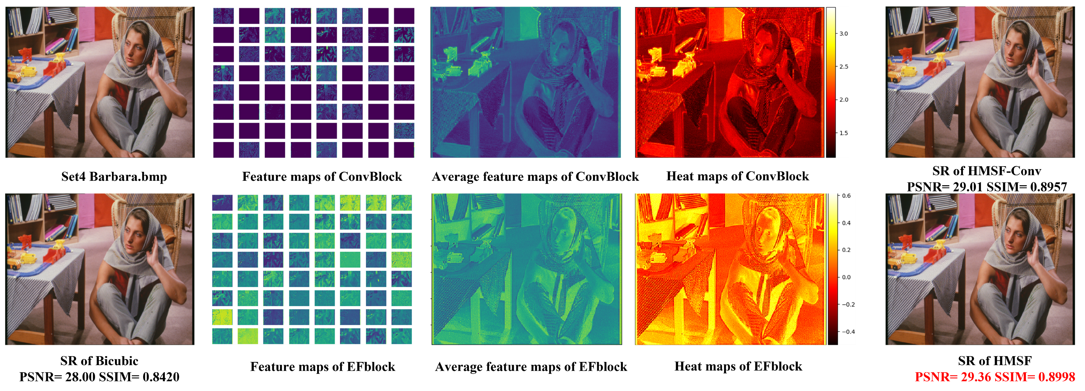
EFblock is an efficient feature extraction block. Compared with the convolution block that consists of two standard 3 × 3 convolutional layers, its parameter number is reduced, but the performance is improved. We designed an ablation experiment by replacing the EFblock with a two-layer 3 × 3 convolutional block similar to that in other methods, similarly aiming to obtain 64-channel features.

Figure 5 shows all 64-dimensional features as well as the heat map of the features, the average features, and the SR image result extracted by Convblock and EFblock when Barbara.bmp in Set14, 2×, is processed. From the total features, it can be seen that the color extracted by the Convblock is dark, and many features are almost black. This shows that these feature maps are not effective; in contrast, the EFblock feature maps include almost all effective knowledge. The heat map makes clear that the features extracted by EFblock are richer, especially the details; furthermore, the color contrast, such as for the several items on the desk, is sharper. The final HMSF-EFblock also yields higher PSNR and SSIM values for Barbara.bmp.

Table 4. The ablation experiment results of EFblock, local multi-scale learning and global multi-scale learning were evaluated on three common datasets of 2× with PSNR/SSIM. Red text means the best performance.

Methods	Parameters	EFB	NST	NMT	Set14	B100	Manga109
HMSF-${}_{\mathit{CONV}}$	732 K	×	√	√	33.77/0.9192	32.27/0.9008	38.87/0.9776
HMSF-${}_{\mathit{NMT}}$	610 K	√	×	√	33.72/0.9186	32.25/0.9007	38.87/0.9776
HMSF-${}_{\mathit{NST}}$	462 K	√	√	×	33.55/0.9170	32.17/0.8996	38.41/0.9768
HMSF	729 K	√	√	√	33.81/0.9194	32.28/0.9009	38.94/0.9778

shows the use of Convblock and EFblock to train the HMSF model. We used 2× three general datasets for testing. The number of parameters of HMSF-EFblock is 3000 less than that of HMSF using Convblock, with fewer multi-adds, too. HMSF-EFblock excels in all three datasets, especially in Manga109 and Set14. The ablation experiment shows that, compared with Convblock, the efficient and lightweight feature-extraction module EFblock has the advantages of a small number of parameters and calculations, while performing quite well.

4.3.2. Study of Local Multi-Scale Learning

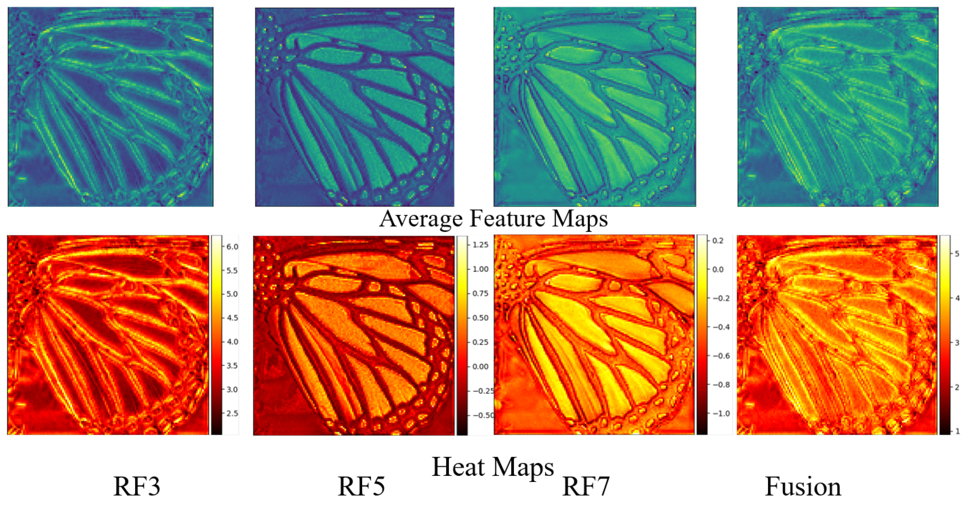
Local multi-scale is mainly used for texture features. Convolutional layers with different receptive fields can extract texture features with different thicknesses and precision. Figure 6 shows the feature maps and heat maps extracted from the RF series of multi-scale modules with different receptive field sizes. It can be seen that, as the receptive field increases, the extracted texture features become more and more concise, from fine details to image contours. The fusion image shows the fusion result of texture features with different levels of fineness: both fine features and rough contours.

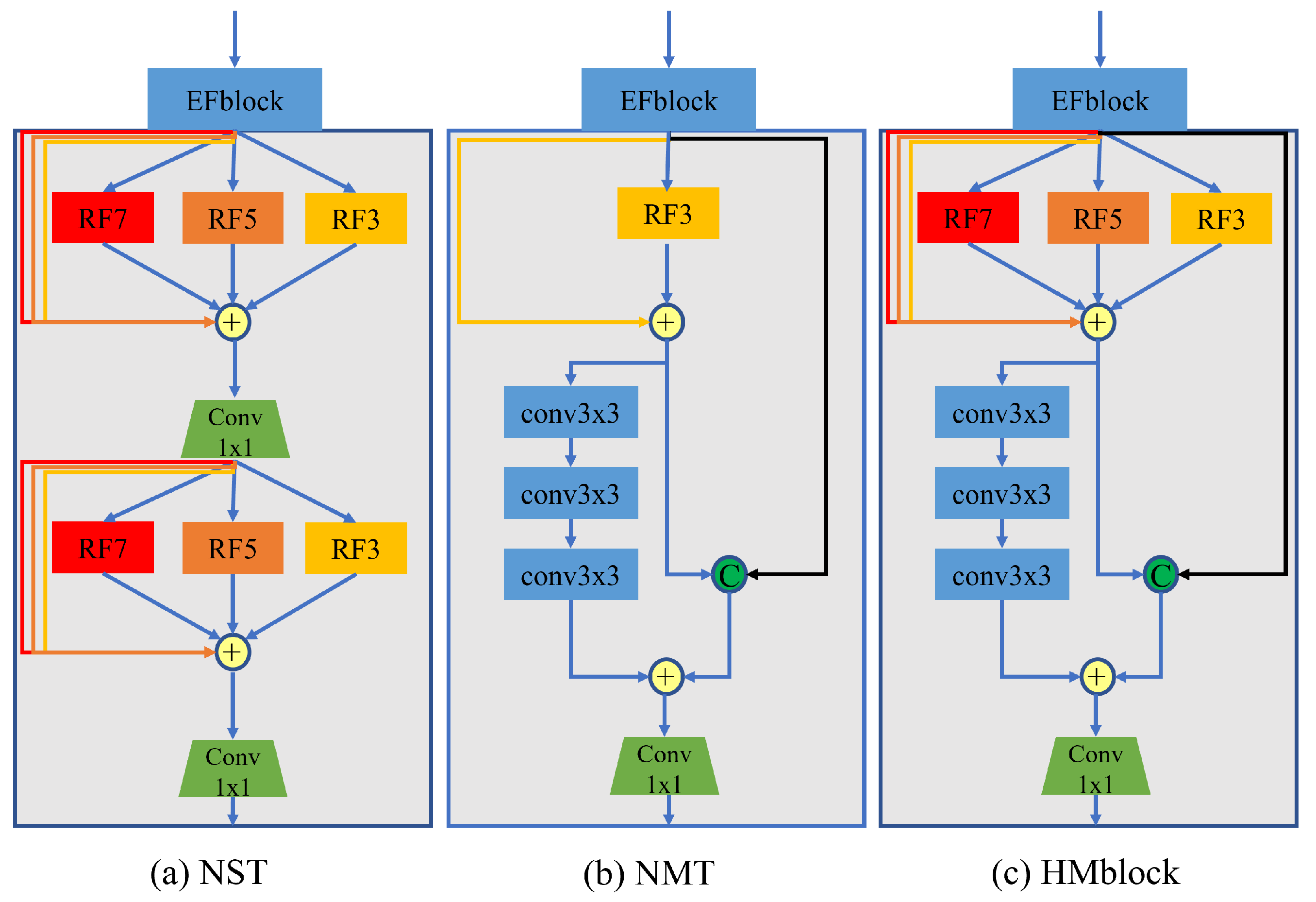
NMT and HMblock in Figure 7 represent the differences between local single-scale and multi-scale texture-extraction structures. We kept the local and global residual connections, and adjusted only the number of local multi-scale modules, RF. The HMSF-NMT in Table 4 represents a model that uses a local single-scale structure during texture extraction. Although the parameters and calculations of the local single-scale structural model are slightly reduced, the performance is greatly reduced, and each test dataset declines. Among them, the decline in Urban100 is the most obvious. Experiments show that local multi-scale texture features are very important for reconstructing local details of the image.

4.3.3. Study of Irregular Convolution

We propose an RF module that uses two types of irregular convolution, dilated convolution and deformable convolution, to obtain different sizes of the receptive field. We view these two irregular convolutions as a whole module; the dilated convolution aims to reach the receptive field, while the deformable convolution aims to extract the irregular feature. To compare our approach with the use of regular convolution, we designed an ablation experiment with five sub experiments: (a) presents the HMSF that, using regular convolutions, has different sizes of kernels (i.e., 3 × 3, 5 × 5, 7 × 7) to obtain different receptive fields; (b) means using stack regular convolution 3 × 3 to achieve the same size of receptive fields; and (c,d) means replacing two types of irregular convolution with regular convolution 3 × 3 in HMblock. Note that DI means dilated convolution, and DE means deformable convolution.

Table 5. The ablation experiment of the use of RC/DI/DE (regular/dilated/deformable convolution). Red text means the best performance.

HMSF	Parameters	Scale	Set14		B100		Manga 109
			PSNR	SSIM	PSNR	SSIM	PSNR	SSIM
(a) RC_based	762 K	2	33.60	0.9174	32.19	0.8999	38.75	0.9772
(b) RC_RC_based	695 K	2	33.71	0.9159	32.25	0.9005	38.77	0.9775
(c) DI_RC_based	675 K	2	33.71	0.9179	32.25	0.9006	38.79	0.9775
(d) RC_DE_based	729 K	2	33.70	0.9158	32.24	0.9005	38.74	0.9775
(e) DI_DE_based	729 K	2	33.81	0.9194	32.28	0.9009	38.94	0.9777

shows a performance comparison between five types of HMSF. It is obvious that, with the factor 2 ×, the comparison between (d) and (e) prove the advance of the use of dilated convolution (DI) by achieving performance improvement on three datasets; on the other hand, it can be seen that using deformable convolution (DE) can achieve better performance through comparing (c) and (e). Moreover, compared to (e) and the traditional RC-based multi-scale method (a), the use of two types of irregular convolutions not only can greatly reduce the number of parameters, but also improve performance and achieve a better PSNR/SSIM on all three datasets.

4.3.4. Study of Global Multi-Scale Learning

Besides local multi-scale texture features, the method also proposes relative global multi-scale structure features. These two scale features constitute global multi-scale features. The two feature maps at the bottom of Figure 3 represent the average feature maps of global multi-scale texture features as well as structural features. The texture features are dark and retain the fine texture features of the baby, hat and other items, while the structural feature only retains the definite outline and the main features of the face and facial organs. The output of the final fusion feature map is texture, accurately registering and reconstructing features and structural features, while yielding effective features with rich thickness, texture and an accurate structure. We conducted ablation experiments on global multi-scale structural features. The NST in Figure 7 indicates that only the local multi-scale texture feature extraction structure was used; the structure feature was not extracted. The trained model is named HMSF-NST. Table 4 shows the greatly reduced performance of HMSF-NST with the global multi-scale structure feature removed; in each dataset, there was significant performance degradation.

4.3.5. Study of Loss Function

Table 6. The performance of models trained with different loss functions.

Loss Function	Scale	Set5	B100
		PSNR (dB)/SSIM	PSNR (dB)/SSIM
L2	2×	38.04/0.9606	32.24/0.9006
Charbonnier (L1)	2×	38.10/0.9609	32.28/0.9009

shows the performance of our model trained with three loss functions, using a factor of 2×, and evaluating it using Set14 and Urban100. Among them, the model trained by Charbonnier loss has better performance than the L2 loss.

4.4. Comparisons with State-of-the-Arts

As shown in

Table 7. Quantitative comparisons (PSNR (DB)/SSIM for 2×, 3× and 4×) of SOTA SR models. Red/blue text means the best/second-best performance.

Model	Scale	Param	Set5	Set14	B100	Urban100	Manga109
SRCNN [15]	2	57 K	36.66/0.9542	32.42/0.9063	31.36/0.8879	29.50/0.8946	35.60/0.9663
FSRCNN [16]	2	12 K	37.00/0.9558	32.63/0.9088	31.53/0.8920	29.88/0.9020	36.67/0.9710
VDSR [17]	2	665 K	37.53/0.9587	3303/0.9124	31.90/0.8960	30.76/0.9140	37.22/0.9750
DRCN [29]	2	1774 K	37.63/0.9588	33.04/0.9118	31.85/0.8942	30.75/0.9133	37.55/0.9732
LapSRN [8]	2	813 K	37.52/0.9590	33.08/0.9130	31.80/0.8950	30.41/0.9100	37.27/0.9740
DRRN [7]	2	297 K	37.74/0.9591	33.23/0.9136	32.05/0.8973	31.23/0.9188	37.88/0.9749
MemNet [9]	2	677 K	37.78/0.9597	33.28/0.9142	32.08/0.8978	31.31/0.9195	37.72/0.9740
EDSRbase [6]	2	1370 K	37.99/0.9604	33.57/0.9175	32.16/0.8994	31.98/0.9272	38.54/0.9769
SRMDNF [56]	2	1513 K	37.79/0.9600	33.32/0.9150	32.05/0.8980	31.33/0.9200	38.07/0.9761
IDN [11]	2	796 K	37.83/0.9600	33.30/0.9148	32.08/0.8985	31.27/0.9196	38.01/0.9749
CARN [10]	2	1592 K	37.76/0.9590	33.52/0.9166	32.09/0.8978	31.92/0.9256	/
DRFN [14]	2	-	37.11/0.9595	33.29/0.9142	32.02/0.8979	31.08/0.9179	/
MADNet [12]	2	878 K	37.85/0.9600	33.39/0.9161	32.05/0.8981	17.59/0.9234	/
LESRCNN [34]	2	626 K	37.65/0.9586	33.32/0.9148	31.95/0.8964	31.45/0.9206	/
CFSRCNN [26]	2	1200 K	37.79/0.9591	33.51/0.9165	32.11/0.8988	32.07/0.9273	/
MRFN [13]	2	-	37.98/0.9611	33.41/0.9159	32.14/0.8997	31.45/0.9221	/
GLADSR [33]	2	812 K	37.99/0.9608	33.63/0.9179	32.16/0.8996	32.16/0.9283	/
HMSF	2	729 K	38.10/0.9609	33.81/0.9194	32.28/0.9009	32.52/0.9322	38.94/0.9777
SRCNN [15]	3	57 K	32.66/0.9089	29.30/0.8215	28.41/0.7863	26.24/0.7989	30.48/0.9117
FSRCNN [16]	3	12 K	33.16/0.9140	29.43/0.8242	28.53/0.79l0	26.43/0.8080	31.10/0.9210
VDSR [17]	3	665 K	33.67/0.9210	29.54/0.8277	28.55/0.7945	26.48/0.8175	32.01/0.9340
DRCN [29]	3	1774 K	33.85/0.9215	29.89/0.8317	28.81/0.7954	27.16/0.8311	32.24/0.9343
LapSRN [8]	3	813 K	33.82/0.9227	29.87/0.8320	28.82/0.7980	27.07/0.8280	32.21/0.9350
DRRN [7]	3	297 K	34.03/0.9244	29.96/0.8349	28.95/0.8004	27.53/0.8378	32.71/0.9379
MemNet [9]	3	677 K	34.09/0.9248	30.00/0.8350	28.96/0.8001	27.56/0.8376	32.71/0.9381
EDSRbase [6]	3	1555 K	34.37/0.9270	30.28/0.8417	29.09/0.8052	28.15/0.8527	33.45/0.9439
SRMDNF [56]	3	1530 K	34.12/0.9254	30.04/0.8370	28.97/0.8030	27.57/0.8400	33.00/0.9403
IDN [11]	3	796 K	34.11/0.9253	29.99/0.8354	28.95/0.8013	27.42/0.8359	32.71/0.9381
CARN [10]	3	1592 K	34.29/0.9255	30.29/0.8407	29.06/0.8034	28.06/0.8493	/
DRFN [14]	3	-	34.01/0.9234	30.06/0.8366	28.93/0.8010	27.43/0.8359	/
MADNet [12]	3	930 K	34.14/0.9251	30.20/0.8395	28.98/0.8023	27.78/0.8439	/
LESRCNN [34]	3	811 K	33.93/0.9231	30.12/0.8380	28.91/0.8005	27.70/0.8415	/
CFSRCNN [26]	3	1200 K	34.34/0.9256	30.27/0.8410	29.03/0.8035	28.04/0.8496	/
MRFN [13]	3	-	34.21/0.9267	30.03/0.8363	28.99/0.8029	27.53/0.8389	/
GLADSR [33]	3	821 K	34.41/0.9272	30.37/0.8418	29.08/0.8050	28.24/0.8537	/
HMSF	3	730 K	34.49/0.9280	30.42/0.8438	29.15/0.8065	28.33/0.8566	33.71/0.9453
SRCNN [15]	4	57 K	30.48/0.8628	27.50/0.7513	26.90/0.7101	24.52/0.7221	27.58/0.8555
FSRCNN [16]	4	12 K	30.73/0.8601	27.71/0.7488	26.98/0.7029	24.62/0.7272	27.90/0.8610
VDSR [17]	4	665 K	31.35/0.8830	28.02/0.7680	27.29/0.7267	25.18/0.7540	28.83/0.8870
DRCN [29]	4	1774 K	31.56/0.8810	28.15/0.7627	27.24/0.7150	25.15/0.7530	28.93/0.8854
LapSRN [8]	4	813 K	31.54/0.8850	28.19/0.7720	27.32/0.7270	25.21/0.7560	29.09/0.8900
DRRN [7]	4	297 K	31.68/0.8888	28.21/0.7720	27.38/0.7284	25.44/0.7638	29.45/0.8946
MemNet [9]	4	677 K	31.74/0.8893	28.26/0.7723	27.40/0.7281	25.50/0.7630	29.42/0.8942
EDSRbase [6]	4	1518 K	32.09/0.8938	28.58/0.7813	27.57/0.7357	26.04/0.7849	30.35/0.9067
SRMDNF [56]	4	1555 K	31.96/0.8930	28.35/0.7770	27.49/0.7340	25.68/0.7730	30.09/0.9024
IDN [11]	4	796 K	31.82/0.8903	28.25/0.7730	27.41/0.7297	25.41/0.7632	29.41/0.8942
CARN [10]	4	1592 K	32.13/0.8937	28.60/0.7806	27.58/0.7349	26.07/0.7837	/
DRFN [14]	4	-	31.55/0.8861	28.30/0.7737	27.39/0.7293	26.45/0.7629	/
MADNet [12]	4	1002 K	32.01/0.8925	28.45/0.7781	28.47/0.7327	25.77/0.7751	/
LESRCNN [34]	4	774 K	31.88/0.8903	28.44/0.7772	27.45/0.7313	25.77/0.7732	/
CFSRCNN [26]	4	1200 K	32.06/0.8920	28.57/0.7800	27.53/0.7333	26.03/0.7824	/
MRFN [13]	4	-	31.90/0.8916	28.31/0.7746	27.43/0.7309	25.46/0.7654	/
GLADSR [33]	4	826 K	32.14/0.8940	28.62/0.7813	27.59/0.7361	26.12/0.7851	/
HMSF	4	731 K	32.15/0.8947	28.61/0.7821	27.61/0.7372	26.15/0.7887	30.52/0.9082

, we compare our proposed HMSF with several state-of-the-art lightweight SR methods, including SRCNN [15], FSRCNN [16], VDSR [17], DRCN [29], LapSRN [8], DRRN [7], IDN [11], CARN [10] and MRFN [13], from 2014 to 2020, with a total of 18 methods. We compare our proposed HMSF on five common datasets, using two common quality evaluation indicators: PSNR and SSIM. To further evaluate the model parameters, memory usage, and multi-adds (Madds), we compare several methods to obtain 1280 × 720 pictures as the benchmark to calculate the above indicators.

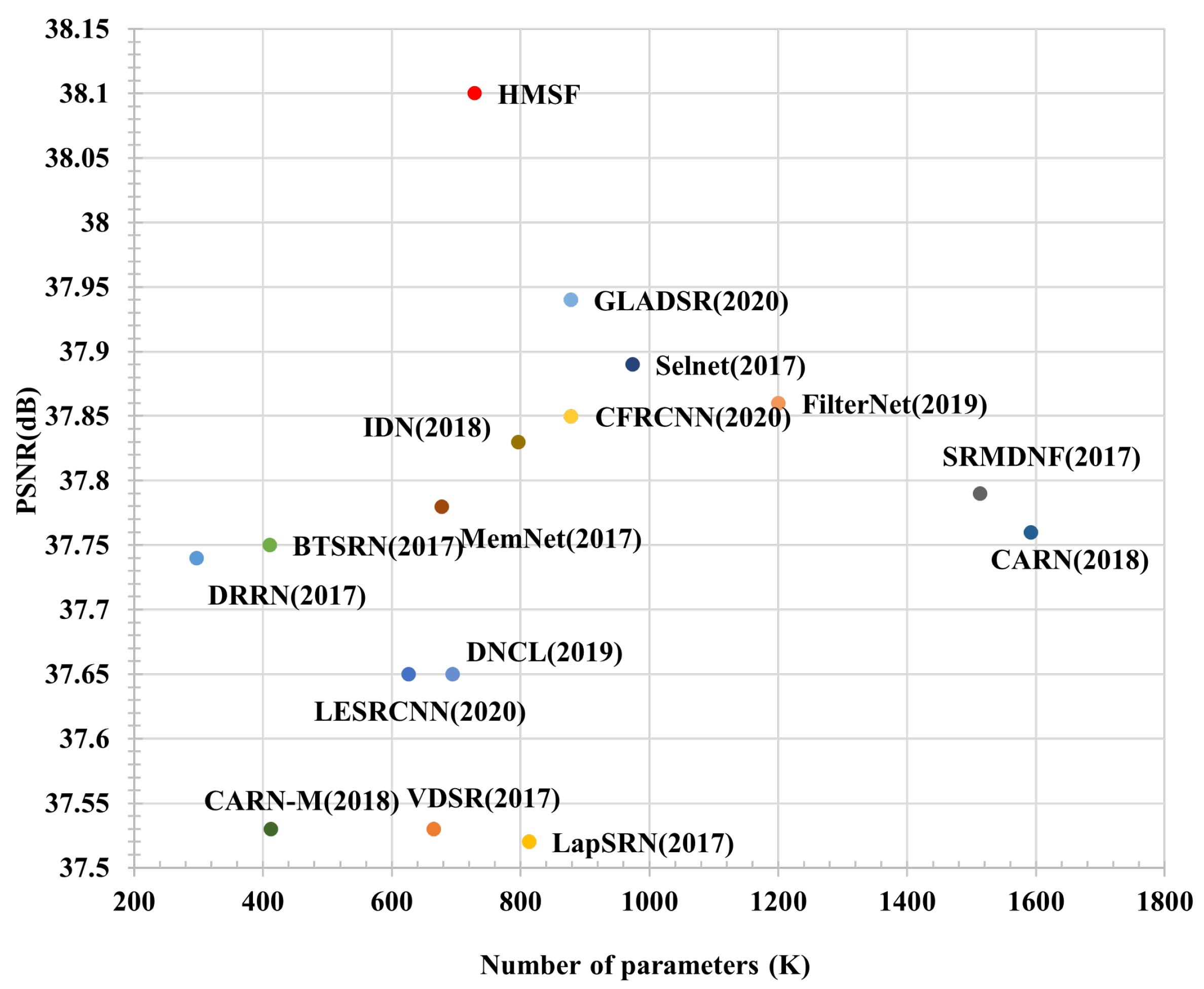
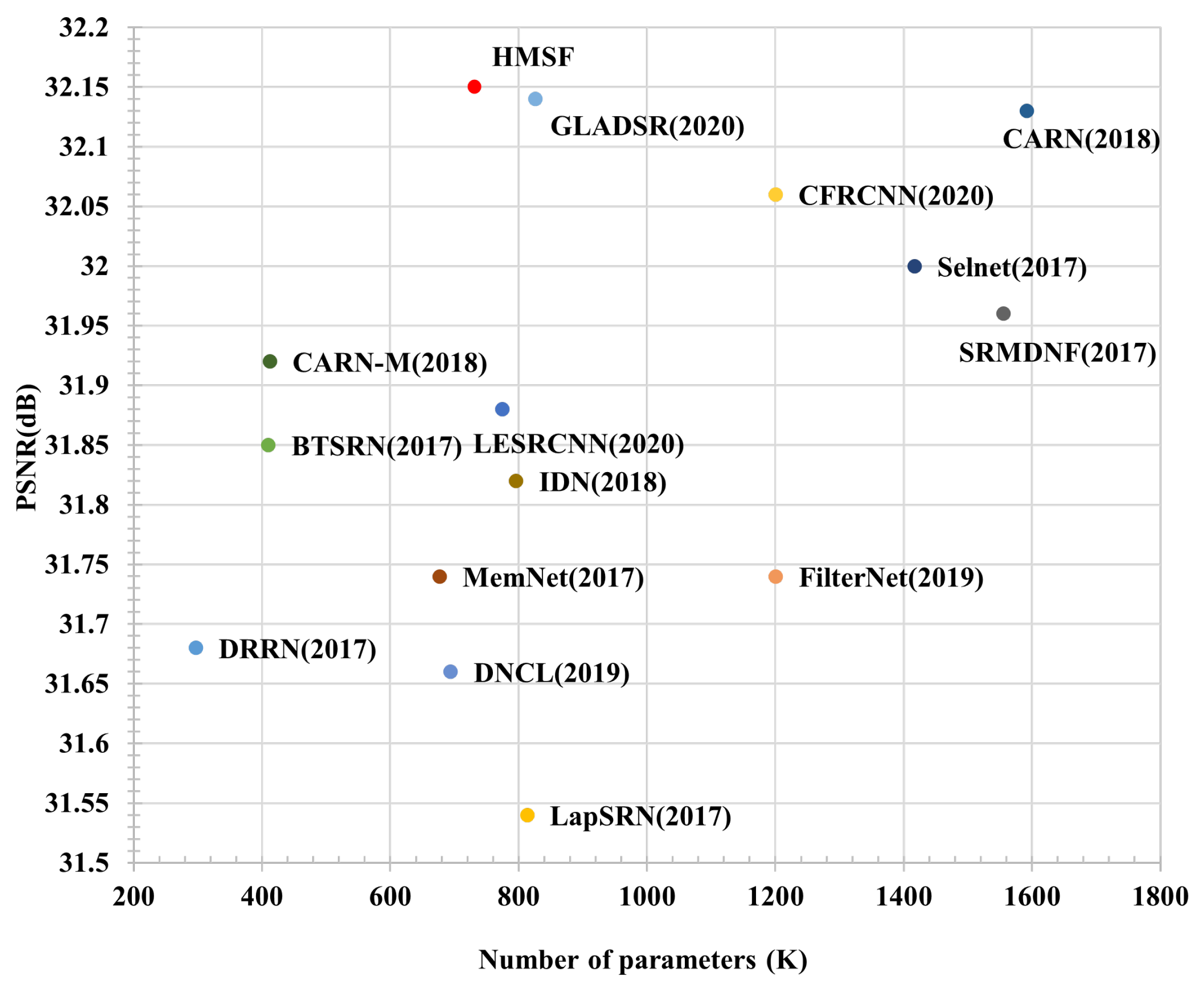
As shown in Figure 8 and Figure 9, compared with some recent methods, ours requires fewer parameters, but performs excellently. Further experiments show that our method bests the existing methods in terms of model size and memory consumption, and exceeds the state-of-the-art method in terms of performance.

Table 8. Comparison of parameters and feature extraction layers of several methods with 2×.

Methods	SRCNN [15]	VDSR [17]	LapSRN [8]	CARN [10]	IDN [11]	MRFN [13]	HMSF
Parameters	57 K	665 K	813 K	1592 K	796 K	-	729 K
Feature Extraction	Conv Layers	Conv Layers	Conv Layers	Conv Layers	Conv Layers	Conv Layers	EFblock
Global Multi-Scale	×	×	×	×	√	×	√
Local Multi-Scale	×	×	√	×	×	√	√
Hybrid Multi-Scale	×	×	×	×	×	×	√

shows the difference between our method and others.

Since our proposed method is based on the idea of hybrid multi-scale features, our method has only two items—Set5 × 2 and Set14 × 4—ranking second among all PSNR and SSIM comparison items, while other items show the best performance. Our method can make the SR image more similar to the original structure and texture of the ground truth image, as well as producing similar results in terms of brightness, contrast, and structure. In the 2× stage, some models come close to ours: EDSR-baseline, MRFN and GLDSR. When compared with the EDSR-baseline, however, we lead in PSNR and SSIM on all datasets, although the parameter number of the EDSR-baseline is about twice that of ours. In comparison with MRFN, Set5’s SSIM is only slightly behind, by 0.003. However, we are far ahead in other aspects, especially in the Set14 and Urban100 datasets. In the Urban100 dataset, our method exceeds the GLADSR on PSNR by 0.36. The Urban100 dataset contains many urban scenes; the texture of houses and streets in the pictures is complex, but the structure is very regular. Because our method focuses on hybrid features-extraction and fusion of texture features and structural features, ours can be better applied to complex scenes. Experimental data also show that our method has advantages. Figure 10 shows a visual comparison. In Urban100’s img067.png image, there are many windows. These windows are structured, which means that their texture features are not rich, although the structure is very prominent. Among the six visualization methods, only ours understands the structural features and produces the least blur. The other methods have many gray areas between panes. As can be seen in another picture, ppt3.bmp from Set14, our method can better restore the letters on the picture, particularly with less blur.

In the 3× stage, our method performs best on PSNR and SSIM. In contrast, other methods, such as MADNet and SRMDNF, perform less well as the image size increases, necessitating a considerable increase in the number of parameters. For example, the parameter number of MADNet exceeds one million at 4×: too much, perhaps, to execute well on devices with limited memory. With our method, on the other hand, the number of parameters always remains at about 730,000—not increasing excessively as the super-resolution ratio changes. For comparison purposes, we selected some images from B100 that contain natural scenes. As shown in Figure 11 in the image ‘14037.png’, our HMSF restores terrestrial details best; moreover, in the image ‘108005.png’, our method excels by restoring the stripe of the tiger more accurately.

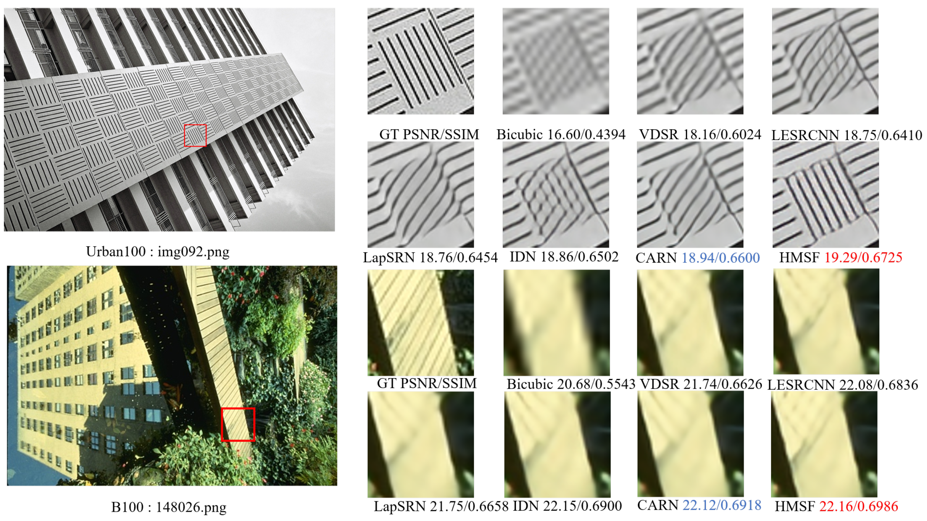
In the 4× stage, our method performs at just a slight disadvantage on Set14. However, methods with performance similar to ours, such as GLADSR, have more parameters, exceeding the number in our method by 95,000. MADNet’s number is also much larger than ours. Figure 12 shows a visual comparison. We chose Urban100’s ‘Img092.png’. In this picture, there are both structured features and rich textures. We notice that, among all six compared methods, almost all of the others reconstruct the numerical texture into an oblique texture. Doing so creates a serious problem, even changing the key structure of the picture. Our method benefits from the fusion of hybrid multi-scale features to better restore the original texture and structure of the graph. The superiority of our method can be seen in yet another picture: ‘148026.png’ in B100. The bridge stripes in this picture, although very rich in texture details, are very subtle and difficult to restore. Only our method can restore more detail this well.

We also compared the models from the perspective of memory usage. With ours, the small number of parameters is a major advantage, directly affecting the memory consumption of the model inference. To keep the comparison fair, we ensured that all methods were experimented with using the same Pytorch platform. As shown in

Table 9. Using memory consumption as the evaluation criterion—in a comparison of five open-source methods with 4× scale—our method has the best performance and smallest memory consumption. Red text means the best performance.

Methods	Scale	Parameters	Set5	Set14	B100	Urban100
			PSNR/SSIM	PSNR/SSIM	PSNR/SSIM	PSNR/SSIM
			Memory	Memory	Memory	Memory
DRRN	4	301 K	31.68/0.8888	28.21/0.7720	27.38/0.7284	25.44/0.7638
			1071 M	1845 M	859 M	8211 M
CARN	4	1592 K	32.13/0.8937	28.60/0.7806	27.58/0.7349	26.07/0.7837
			803 M	983 M	695 M	2697 M
EDSR-baseline	4	1518 K	32.09/0.8938	28.58/0.7813	27.57/0.7357	26.04/0.7849
			727 M	921 M	659 M	2497 M
LESRCNN	4	774 K	31.88/0.8903	28.44/0.7772	27.45/0.7313	25.77/0.7732
			1149 M	1805 M	903 M	7307 M
HMSF	4	731 K	32.15/0.8947	28.61/0.7821	27.61/0.7372	26.15/0.7887
			652 M	729 M	611 M	1854 M

, we used four datasets for evaluation at a scale of 4×, and recorded memory consumption during inference. We selected several open-source representative methods: (1) DRRN, with the number of parameters much smaller than ours; (2) CARN, with the number of parameters much larger than ours; and (3) EDSR-baseline and LESRCNN, with a number of parameters similar to ours. It can be seen that DRRN, despite its small number of parameters, required very large memory consumption, reaching 8211 MB on the Urban100 dataset—too much for most personal computers. Several other methods performed satisfactorily, but consumed more than 2 GB of memory on the Urban100 dataset, more than can be supported by personal computers and mobile devices. Our method consumed the least memory for each dataset, but achieved satisfactory performance, especially on the Urban100 dataset; our memory consumption was about 800 MB lower than CARN’s, while our PSNR was 0.08 higher, and our SSIM was 0.005 higher. As shown in Figure 13, compared with four SOTAs, the proposed model achieves the best performance with less memory consumption in Urban100 4×.

We further add the comparisons between multi-scale-based SOTAs [12,13,57,58]. Among them, Wang et al. proposed a traditional theory-based multi-scale method that uses multi-scale dictionary training to construct the mapping of SR and LR. On the other hand, MADNet, MRFN, and the method proposed by Du et al. consider regular convolutions with different kernel sizes to obtain multi-scale receptive fields.

Table 10. Quantitative comparisons (PSNR (DB)/SSIM for 3×) of SOTA multi-scale-based SR models. Red text means the best performance.

Method	Multi-Scale Implementation	Scale	Set5	Set14
Wang et al. [57]	Multi-Scale Dictionary	3	33.40/0.9200	29.51/0.8300
Du et al. [58]	Regular Convolution	3	33.44/0.9185	29.59/0.9290
MADNet [12]	Regular Convolution	3	34.14/0.9250	30.20/0.8390
MRFN [13]	Regular Convolution	3	34.21/0.9260	30.03/0.8360
HMSF (ours)	Dilated + Deformable Convolution	3	34.49/0.9280	30.42/0.8438

shows that the CNN-based methods achieve better performance than the traditional theory-based method. What is more, our HMSF is based on dilated convolutions and deformable convolutions, which leads to a more powerful ability to learn multi-scale features and achieves better performance in both Set5 and Set14 than other methods based on regular convolutions.

In addition, we compared several open-source methods with similar parameters.

Table 11. Multi-adds compared between six similar methods at 4× scale. Madds evaluated the number of multiplications and additions of the model, and evaluated the combination of parameters and Madds. Red text means the best performance.

Methods	Scale	Parameters	Madds	Set14	B100	Urban100
				PSNR/SSIM	PSNR/SSIM	PSNR/SSIM
LapSRN	4	813 K	149 G	28.19/0.7720	27.32/0.7270	25.21/0.7560
MemNet	4	677 K	2662 G	28.26/0,7723	27.40/0.7281	25.50/0.7630
CARN	4	1592 K	90 G	28.60/0.7806	27.58/0.7349	26.07/0.7837
MADNet	4	1002 K	54 G	28.45/0.7781	27.47/0.7327	25.77/0.7751
LESRCNN	4	774 K	241 G	28.44/0.7772	27.45/0.7313	25.77/0.7732
HMSF	4	731 K	122 G	28.61/0.7821	27.61/0.7372	26.15/0.7887

shows a comparison of our multi-adds with the performance of several methods with similar parameters. Generally speaking, the number of parameters affects memory usage during execution, to a certain extent. Multi-adds can reflect execution speed. We can see that CARN, the second method listed in the table, had slightly fewer multi-adds, but its number of parameters was greatly increased, with performance much lower than ours. Although MemNet had fewer parameters, its number of multi-adds was excessive: tens of times more than those of other methods. For LESRCNN, the number of parameters and multi-adds was slightly larger than ours, but its performance was poor. In general, our method requires moderate parameters and calculations, but provides satisfactory performance. For example, our number of parameters was 861,000 fewer than that of CARN. While our number of multi-adds was increased by only 32 G, the performance of our method exceeded that of CARN on all three datasets, especially on Urban100, for which the PSNR was increased by 0.08.

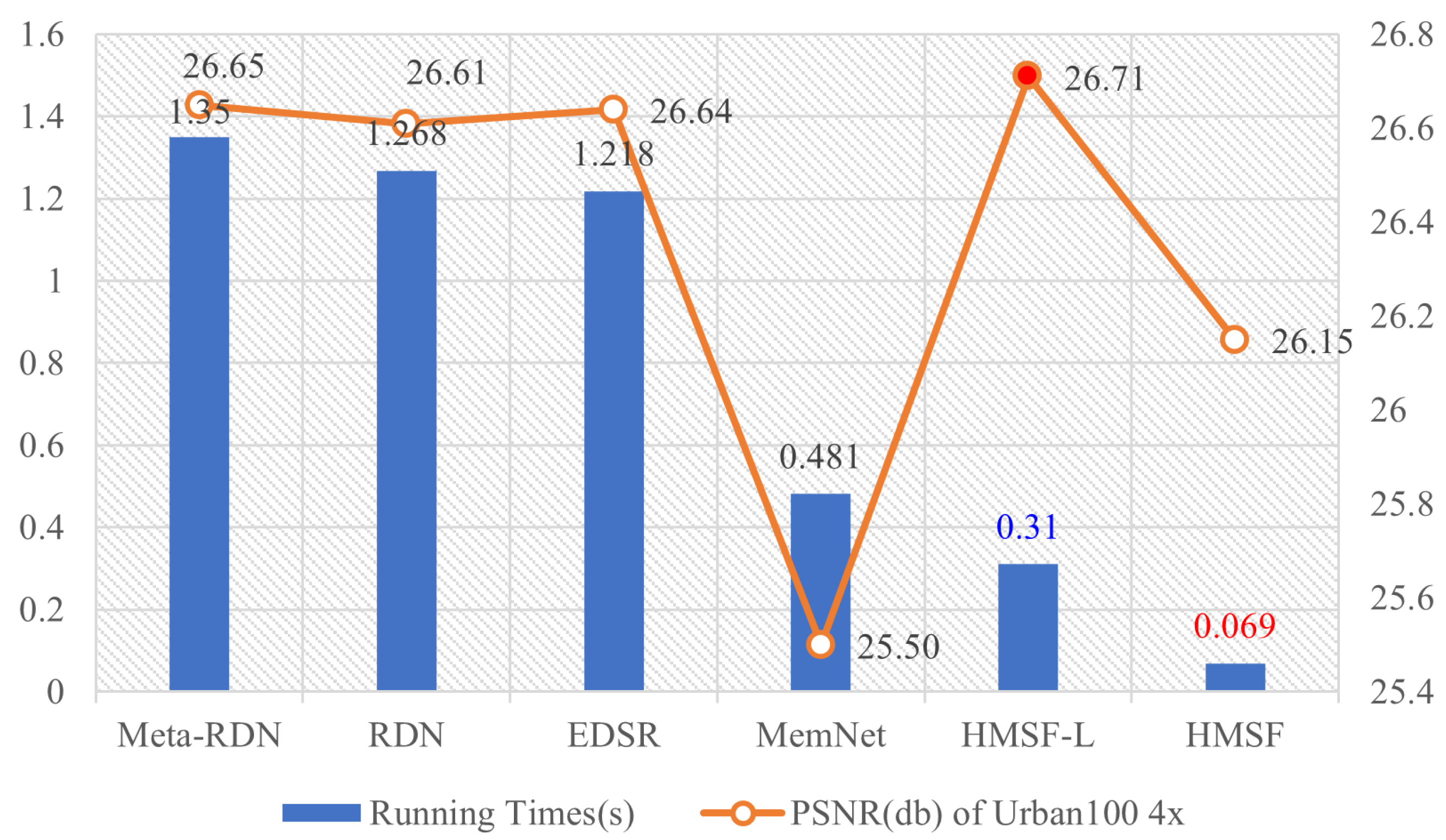
Moreover, we added a comparison about the run times with several state-of-the-art methods [6,9,59,60]; in keeping with some recent research [61], we used the same GPU (Nvidia GTX 1080 Ti) to run models including HMSF and HMSF-L, and processed 100 images from Urban100 for 4×.

Table 12. Comparison of average running time on Urban100 for 4×. Red/blue text means the best/second-best performance.

Model	Parameters	Running Times (s)	PSNR	SSIM
MemNet	0.6 M	0.481	25.50	0.7630
EDSR	43 M	1.218	26.64	0.8029
RDN	22 M	1.268	26.61	0.8028
Meta-RDN	22 M	1.35	26.65	-
HMSF (Ours)	0.7 M	0.069	26.15	0.7887
HMSF-L (Ours)	4.48M	0.31	26.71	0.8056

and Figure 14 show that, compared with four state-of-the-art methods, our HMSF ran the fastest; HMSF-L had the second-best speed. HMSF-L achieved better image quality with higher PSNR/SSIM, meaning that HMSF-L achieved both efficiency and accuracy.

4.5. Further Comparisons with Larger State-of-the-Art Methods

Although our HMSF provides the benefits of being lightweight and effective, we designed a series of comparisons to further demonstrate its potential. Given that our model initially aimed to build a lightweight and tight neural network architecture, we preferred to keep our original network structure, and simply changed the number of channels in some layers to add parameters in order to enlarge the model size. We enlarged our HMSF to middle size and named it HMSF-L. To enlarge it, we increased the number of blocks to three, and applied more channels. We selected five state-of-the-art methods, including SRDenseNet [62], EDSR [6], FRSR [63], SRGAN [64], and NatSR [63]; most have a similar number of parameters. As shown in

Table 13. We enlarge the HMSF to a middle size, and compare it with other state-of-the-art models that have a similar number of parameters. Red/blue text means the best/second-best performance.

Dataset	Scale	SRDenseNet		EDSR		FRSR		SRGAN		NatSR		HMSF-L
		PSNR	SSIM	PSNR	SSIM	PSNR	SSIM	PSNR	SSIM	PSNR	SSIM	PSNR	SSIM
Set5	4	32.02	0.8934	32.46	0.8968	32.20	0.8939	29.41	0.8345	30.98	0.8606	32.44	0.8987
Set14	4	28.50	0.7782	28.80	0.7876	28.54	0.7808	26.02	0.6934	25.67	0.6757	28.82	0.7876
B100	4	27.53	0.7337	27.71	0.7420	27.60	0.7366	25.18	0.6401	24.93	0.6259	27.75	0.7428
Urban100	4	26.05	0.7819	26.64	0.8033	26.21	0.7904	/	/	23.54	0.6926	26.71	0.8056
Parameters	4	2.0 M		43 M		4.8 M		1.5 M		4.8 M		4.48 M

, our HMSF-L has a middle size, includes 4.48 million parameters, and achieved strong performance. HMSF-L achieved the best scores on seven comparative items with a 4× factor; compared to the second-best method, EDSR, our model trailed behind only Set5 with a PSNR of 0.02, but with far fewer parameters—those of EDSR were almost 9.6 times more than ours with HMSF-L. Furthermore, to compare ours with other state-of-the-art methods designed with a large size, we enlarged our HMSF to a larger size, named HMSF-XL, by simply increasing the number of HMblocks to five and further increasing the channels in some layers. As a result, our model’s number of parameters was increased to 15.4 million. Since any model with more than 15 million parameters can be categorized as a standard large model, we selected five state-of-the-art methods, most with more than 15 million parameters. The five include EDSR [6], SRGAT [65], RDN [59], RCAN [66] and SAN [67]; at least four of them require more parameters than our HMSF-XL. For comparison, we evaluated the methods on four common datasets. To fairly and comprehensively compare them, we considered average PSNR/SSIM as well as the number of parameters. As shown in

Table 14. We enlarge the HMSF to a large size, and compare it with other state-of-the-art models that have a similar number of parameters. Red/blue text means the best/second-best performance.

Dataset	Scale	EDSR		SRGAT		RDN		RCAN		SAN		HMSF-XL
		PSNR	SSIM	PSNR	SSIM	PSNR	SSIM	PSNR	SSIM	PSNR	SSIM	PSNR	SSIM
Set5	2	38.11	0.9601	38.20	0.9610	38.24	0.9614	38.27	0.9614	38.31	0.9620	38.28	0.9616
Set14	2	33.92	0.9195	33.93	0.9201	34.01	0.9212	34.12	0.9216	34.07	0.9213	34.13	0.9219
B100	2	32.32	0.9013	32.34	0.9014	32.34	0.9017	32.41	0.9027	32.42	0.9028	32.40	0.9026
Urban100	2	32.93	0.9351	32.90	0.9359	32.89	0.9353	33.34	0.9384	33.10	0.9370	33.20	0.9384
Avarage	2	34.32	0.9290	34.34	0.9296	34.37	0.9299	34.54	0.9310	34.48	0.9308	34.50	0.9311
Parameters		43 M		/		22.3 M		16 M		15.7 M		15.4 M

with the three methods RCAN, SAN and our HMSF-XL, each displayed certain advantages. RCAN performed better than HMSF-XL on 4 out of 11 items. At best—on Urban100—RCAN outperformed our method with a PSNR of 0.14 db. On the other hand, HMSF-XL achieved better performance on 6 of the 11 items. Moreover, compared to SAN, our HMSF-XL performed better on 7 of the 11; furthermore, SAN failed to placed first or second in performance on 4 of the 11, even with 0.3 million more parameters than ours. In summary, our HMSF-XL was enlarged simply by increasing the number of channels in some network layers, without modifying the main architecture of the network. Obviously, there were several methods that performed better than our HMSF-XL on some items, but on most items, our method excelled. In short, HMSF-XL provides better overall performance with a small number of parameters.

4.6. Further Test on Real-World Images

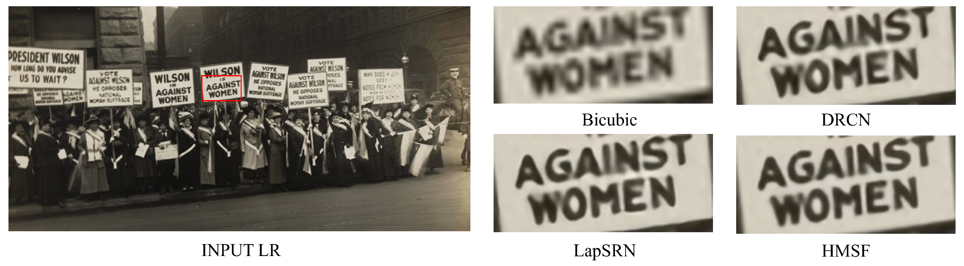
As a powerful image processing tool, super-resolution is widely used. In the real world, however, there are few LR-HR image pairs that can be evaluated for image quality. To simulate a real-world scenario, we followed the methods described in [8,56], using some real-world images to test ours. Because there are no HR images that suit these real-world images, we provided just the visualized results to be evaluated. Figure 15 shows a real-world historical image, processed with factor 2×; in the visualized comparison, it can be detected that our HMSF restored font details better. Figure 16 shows a visualized test result on the real LR image, Cat.png, which was more difficult to process because of its blur. Compared to the results of LapSRN [8], Waifu2x [68] and CARN [10], the image processed by HMSF appears with a sharper edge as well as a purer black color.

4.7. Analysis of Limitations

As previously mentioned, our HMSF achieves better performance in terms of PSNR/ SSIM and visualization quality. However, many deep-learning-based models [10,11,17,34] (including our HMSF) share a problem, as shown in Figure 17: none of the methods can correctly restore the direction of a stripe from the input of a bicubic low-resolution image. In a bicubic image, stripes are displayed as staggered black and white pixels; each white/black pixel connects the next black/white pixel in two contrary directions. Such a phenomenon will mislead trained models to yield undesirable results.

5. Discussion

In light of the paper, our proposed HMSF is lightweight, accurate, and fast, and has fewer parameters but performs better than SOTAs. We found that existing lightweight methods ignore the texture and structural characteristics of features and do not effectively extract them, which leads to an unsatisfying image restore quality. To tackle the aforementioned problem, we proposed an efficient feature extraction module and a hybrid multi-scale mechanism that aims to efficiently extract multi-level image structure and texture features. Unlike previous multi-scale mechanisms, our proposed method combines local and global multi-scale features, including both local multi-scale receptive fields and global multi-scale over network depth. Further, in the super-resolution task, the processed images often have blurry and irregular artifacts, which cannot be recovered well by previous methods. To solve this problem, we consider the use of dilated convolution and deformed convolution to further improve the ability to extract local multi-scale texture features. Since the size of the receptive field of deformed convolution is irregular, it is well adapted to complex irregularities artifacts. However, there are also some unsolved problems sustained, as Section 4.7 shows that existing SOTAs cannot correctly restore the direction of stripes in Figure 17, which is a research gap for how to properly fix images with misleading information. We believe that some prior knowledge must be added to guide the model to identify misleading information (i.e., wrong texture orientation) when processing such images. In future research, we will try to incorporate priors that verify misleading information (such as probabilistic predictions of the correct orientation of the texture) in our HMSF to better recover these images with misleading or redundant information.

6. Conclusions

In this paper, we propose a lightweight and fast super-resolution method, based on hybrid multi-scale features. We developed a feature-extraction module, EFblock, with a novel structure, flexible use of point convolution, and grouped convolution. It also adds local and global residual connections, but with fewer parameters—fewer than in the usual convolutional layer. We also propose a novel, hybrid, multi-scale features-extraction block, HMblock, with an efficient bottleneck structure, dilated convolution and deformable convolution, all to achieve local and global multi-scale learning. This can accurately match an image structure, and completely restore texture details. Compared with other state-of-the-art methods, ours performed competitively on five datasets, performing with high efficiency while still being lightweight. In particular, our method necessitates fewer parameters and consumes less memory during execution, yet performs better; in particular, our method offers promising benefits for memory-constrained devices. In further work, we hope to develop a lightweight and efficient video-data super-resolution method. Due to the similarities and differences of tasks, we hope to incorporate associated video frame information into our work so that video super-resolution also can be executed on memory-constrained devices.

References

- Yang, W.; Zhang, X.; Tian, Y.; Wang, W.; Xue, J.; Liao, Q. Deep Learning for Single Image Super-Resolution: A Brief Review. IEEE Trans. Multimed. 2019, 21, 3106–3121. [Google Scholar] [CrossRef] [Green Version]
- Schulter, S.; Leistner, C.; Bischof, H. Fast and accurate image upscaling with super-resolution forests. In Proceedings of the IEEE Conference on Computer Vision and Pattern Recognition, Boston, MA, USA, 7–12 June 2015; pp. 3791–3799. [Google Scholar]
- Yang, C.Y.; Yang, M.H. Fast direct super-resolution by simple functions. In Proceedings of the IEEE International Conference on Computer Vision, Sydney, Australia, 1–8 December 2013; pp. 561–568. [Google Scholar]
- Timofte, R.; De Smet, V.; Van Gool, L. A+: Adjusted anchored neighborhood regression for fast super-resolution. In Asian Conference on Computer Vision; Springer: Berlin/Heidelberg, Germany, 2014; pp. 111–126. [Google Scholar]
- Yao, X.; Wu, Q.; Zhang, P.; Bao, F. Weighted Adaptive Image Super-Resolution Scheme based on Local Fractal Feature and Image Roughness. IEEE Trans. Multimed. 2020, 23, 1426–1441. [Google Scholar] [CrossRef]
- Lim, B.; Son, S.; Kim, H.; Nah, S.; Mu Lee, K. Enhanced deep residual networks for single image super-resolution. In Proceedings of the IEEE Conference on Computer Vision and Pattern Recognition Workshops, Honolulu, HI, USA, 21–26 July 2017; pp. 136–144. [Google Scholar]
- Tai, Y.; Yang, J.; Liu, X. Image super-resolution via deep recursive residual network. In Proceedings of the IEEE Conference on Computer Vision and Pattern Recognition, Honolulu, HI, USA, 21–26 July 2017; pp. 3147–3155. [Google Scholar]
- Lai, W.S.; Huang, J.B.; Ahuja, N.; Yang, M.H. Deep laplacian pyramid networks for fast and accurate super-resolution. In Proceedings of the IEEE Conference on Computer Vision and Pattern Recognition, Honolulu, HI, USA, 21–26 July 2017; pp. 624–632. [Google Scholar]
- Tai, Y.; Yang, J.; Liu, X.; Xu, C. Memnet: A persistent memory network for image restoration. In Proceedings of the IEEE International Conference on Computer Vision, Venice, Italy, 22–29 October 2017; pp. 4539–4547. [Google Scholar]
- Ahn, N.; Kang, B.; Sohn, K.A. Fast, accurate, and lightweight super-resolution with cascading residual network. In Proceedings of the European Conference on Computer Vision (ECCV), Munich, Germany, 8–14 September 2018; pp. 252–268. [Google Scholar]
- Hui, Z.; Wang, X.; Gao, X. Fast and accurate single image super-resolution via information distillation network. In Proceedings of the IEEE Conference on Computer Vision and Pattern Recognition, Salt Lake City, UT, USA, 18–22 June 2018; pp. 723–731. [Google Scholar]
- Lan, R.; Sun, L.; Liu, Z.; Lu, H.; Pang, C.; Luo, X. MADNet: A Fast and Lightweight Network for Single-Image Super Resolution. IEEE Trans. Cybern. 2020, 51, 1443–1453. [Google Scholar] [CrossRef]
- He, Z.; Cao, Y.; Du, L.; Xu, B.; Yang, J.; Cao, Y.; Tang, S.; Zhuang, Y. Mrfn: Multi-receptive-field network for fast and accurate single image super-resolution. IEEE Trans. Multimed. 2019, 22, 1042–1054. [Google Scholar] [CrossRef]
- Yang, X.; Mei, H.; Zhang, J.; Xu, K.; Yin, B.; Zhang, Q.; Wei, X. Drfn: Deep recurrent fusion network for single-image super-resolution with large factors. IEEE Trans. Multimed. 2019, 21, 328–337. [Google Scholar] [CrossRef] [Green Version]
- Dong, C.; Loy, C.C.; He, K.; Tang, X. Learning a deep convolutional network for image super-resolution. In European Conference on Computer Vision; Springer: Berlin/Heidelberg, Germany, 2014; pp. 184–199. [Google Scholar]
- Dong, C.; Loy, C.C.; Tang, X. Accelerating the super-resolution convolutional neural network. In European Conference on Computer Vision; Springer: Berlin/Heidelberg, Germany, 2016; pp. 391–407. [Google Scholar]
- Kim, J.; Kwon Lee, J.; Mu Lee, K. Accurate image super-resolution using very deep convolutional networks. In Proceedings of the IEEE Conference on Computer Vision and Pattern Recognition, Las Vegas, NV, USA, 27–30 June 2016; pp. 1646–1654. [Google Scholar]
- Zhang, D.; Shao, J.; Liang, Z.; Gao, L.; Shen, H.T. Large Factor Image Super-Resolution with Cascaded Convolutional Neural Networks. IEEE Trans. Multimed. 2020, 23, 2172–2184. [Google Scholar] [CrossRef]
- Szegedy, C.; Liu, W.; Jia, Y.; Sermanet, P.; Reed, S.; Anguelov, D.; Erhan, D.; Vanhoucke, V.; Rabinovich, A. Going deeper with convolutions. In Proceedings of the IEEE Conference on Computer Vision and Pattern Recognition, Boston, MA, USA, 7–12 June 2015; pp. 1–9. [Google Scholar]
- Yu, F.; Koltun, V. Multi-scale context aggregation by dilated convolutions. arXiv 2015, arXiv:1511.07122. [Google Scholar]
- Dai, J.; Qi, H.; Xiong, Y.; Li, Y.; Zhang, G.; Hu, H.; Wei, Y. Deformable convolutional networks. In Proceedings of the IEEE International Conference on Computer Vision, Venice, Italy, 22–29 October 2017; pp. 764–773. [Google Scholar]
- Riaz, M.; Smarandache, F.; Firdous, A.; Fakhar, A. On soft rough topology with multi-attribute group decision making. Mathematics 2019, 7, 67. [Google Scholar] [CrossRef] [Green Version]
- Khan, N.; Yaqoob, N.; Shams, M.; Gaba, Y.U.; Riaz, M. Solution of Linear and Quadratic Equations Based on Triangular Linear Diophantine Fuzzy Numbers. J. Funct. Spaces 2021, 2021, 8475863. [Google Scholar] [CrossRef]
- Mahmood, T.; Ali, Z.; Aslam, M.; Chinram, R. Generalized Hamacher Aggregation Operators Based on Linear Diophantine Uncertain Linguistic Setting and Their Applications in Decision-Making Problems. IEEE Access 2021, 9, 126748–126764. [Google Scholar]
- Shi, W.; Caballero, J.; Huszár, F.; Totz, J.; Aitken, A.P.; Bishop, R.; Rueckert, D.; Wang, Z. Real-time single image and video super-resolution using an efficient sub-pixel convolutional neural network. In Proceedings of the IEEE Conference on Computer Vision and Pattern Recognition, Las Vegas, NV, USA, 27–30 June 2016; pp. 1874–1883. [Google Scholar]
- Tian, C.; Xu, Y.; Zuo, W.; Zhang, B.; Fei, L.; Lin, C.W. Coarse-to-fine CNN for image super-resolution. IEEE Trans. Multimed. 2020, 23, 1489–1502. [Google Scholar] [CrossRef]
- Wei, W.; Feng, G.; Zhang, Q.; Cui, D.; Zhang, M.; Chen, F. Accurate single image super-resolution using cascading dense connections. Electron. Lett. 2019, 55, 739–742. [Google Scholar] [CrossRef]
- Jin, Z.; Iqbal, M.Z.; Bobkov, D.; Zou, W.; Li, X.; Steinbach, E. A Flexible Deep CNN Framework for Image Restoration. IEEE Trans. Multimed. 2020, 22, 1055–1068. [Google Scholar] [CrossRef]
- Kim, J.; Kwon Lee, J.; Mu Lee, K. Deeply-recursive convolutional network for image super-resolution. In Proceedings of the IEEE Conference on Computer Vision and Pattern Recognition, Las Vegas, NV, USA, 27–30 June 2016; pp. 1637–1645. [Google Scholar]
- Liu, P.; Zhang, H.; Zhang, K.; Lin, L.; Zuo, W. Multi-level wavelet-CNN for image restoration. In Proceedings of the IEEE Conference on Computer Vision and Pattern Recognition Workshops, Salt Lake City, UT, USA, 18–22 June 2018; pp. 773–782. [Google Scholar]
- Li, M.; Zhang, Z.; Yu, J.; Chen, C.W. Learning Face Image Super-Resolution through Facial Semantic Attribute Transformation and Self-Attentive Structure Enhancement. IEEE Trans. Multimed. 2021, 23, 468–483. [Google Scholar] [CrossRef]
- Ahn, N.; Kang, B.; Sohn, K.A. Efficient Deep Neural Network for Photo-realistic Image Super-Resolution. arXiv 2019, arXiv:1903.02240. [Google Scholar]
- Zhang, X.; Gao, P.; Liu, S.; Zhao, K.; Li, G.; Yin, L.; Chen, C.W. Accurate and efficient image super-resolution via global-local adjusting dense network. IEEE Trans. Multimed. 2020, 23, 1924–1937. [Google Scholar] [CrossRef]
- Tian, C.; Zhuge, R.; Wu, Z.; Xu, Y.; Zuo, W.; Chen, C.; Lin, C.W. Lightweight image super-resolution with enhanced CNN. Knowl.-Based Syst. 2020, 205, 106235. [Google Scholar] [CrossRef]
- Iandola, F.N.; Han, S.; Moskewicz, M.W.; Ashraf, K.; Dally, W.J.; Keutzer, K. SqueezeNet: AlexNet-level accuracy with 50x fewer parameters and< 0.5 MB model size. arXiv 2016, arXiv:1602.07360. [Google Scholar]
- Zhang, X.; Zhou, X.; Lin, M.; Sun, J. Shufflenet: An extremely efficient convolutional neural network for mobile devices. In Proceedings of the IEEE Conference on Computer Vision and Pattern Recognition, Salt Lake City, UT, USA, 18–22 June 2018; pp. 6848–6856. [Google Scholar]
- Ma, N.; Zhang, X.; Zheng, H.T.; Sun, J. Shufflenet v2: Practical guidelines for efficient cnn architecture design. In Proceedings of the European Conference on Computer Vision (ECCV), Munich, Germany, 8–14 September 2018; pp. 116–131. [Google Scholar]
- Krizhevsky, A.; Sutskever, I.; Hinton, G.E. Imagenet classification with deep convolutional neural networks. Adv. Neural Inf. Process. Syst. 2012, 25, 1097–1105. [Google Scholar] [CrossRef]
- Howard, A.G.; Zhu, M.; Chen, B.; Kalenichenko, D.; Wang, W.; Weyand, T.; Andreetto, M.; Adam, H. Mobilenets: Efficient convolutional neural networks for mobile vision applications. arXiv 2017, arXiv:1704.04861. [Google Scholar]
- Sandler, M.; Howard, A.; Zhu, M.; Zhmoginov, A.; Chen, L.C. Mobilenetv2: Inverted residuals and linear bottlenecks. In Proceedings of the IEEE Conference on Computer Vision and Pattern Recognition, Salt Lake City, UT, USA, 18–22 June 2018; pp. 4510–4520. [Google Scholar]
- Howard, A.; Sandler, M.; Chu, G.; Chen, L.C.; Chen, B.; Tan, M.; Wang, W.; Zhu, Y.; Pang, R.; Vasudevan, V.; et al. Searching for mobilenetv3. In Proceedings of the IEEE/CVF International Conference on Computer Vision, Seoul, Korea, 27–28 October 2019; pp. 1314–1324. [Google Scholar]
- Zoph, B.; Le, Q.V. Neural architecture search with reinforcement learning. arXiv 2016, arXiv:1611.01578. [Google Scholar]
- Ioffe, S.; Szegedy, C. Batch normalization: Accelerating deep network training by reducing internal covariate shift. arXiv 2015, arXiv:1502.03167. [Google Scholar]
- Szegedy, C.; Vanhoucke, V.; Ioffe, S.; Shlens, J.; Wojna, Z. Rethinking the inception architecture for computer vision. In Proceedings of the IEEE Conference on Computer Vision and Pattern Recognition, Las Vegas, NV, USA, 27–30 June 2016; pp. 2818–2826. [Google Scholar]
- Xie, C.; Zeng, W.; Lu, X. Fast Single-Image Super-Resolution via Deep Network With Component Learning. IEEE Trans. Circuits Syst. Video Technol. 2018, 29, 3473–3486. [Google Scholar] [CrossRef]
- Li, F.; Bai, H.; Zhao, Y. FilterNet: Adaptive information filtering network for accurate and fast image super-resolution. IEEE Trans. Circuits Syst. Video Technol. 2019, 30, 1511–1523. [Google Scholar] [CrossRef]
- Choi, J.S.; Kim, M. A deep convolutional neural network with selection units for super-resolution. In Proceedings of the IEEE Conference on Computer Vision and Pattern Recognition Workshops, Honolulu, HI, USA, 21–26 July 2017; pp. 154–160. [Google Scholar]
- Agustsson, E.; Timofte, R. Ntire 2017 challenge on single image super-resolution: Dataset and study. In Proceedings of the IEEE Conference on Computer Vision and Pattern Recognition Workshops, Honolulu, HI, USA, 21–26 July 2017; pp. 126–135. [Google Scholar]
- Bevilacqua, M.; Roumy, A.; Guillemot, C.; Alberi-Morel, M.L. Low-Complexity Single-Image Super-Resolution Based on Nonnegative Neighbor Embedding. In Proceedings of the British Machine Vision Conference, Guildford, UK, 3–7 September 2012; pp. 135.1–135.10. [Google Scholar]
- Yang, J.; Wright, J.; Huang, T.S.; Ma, Y. Image super-resolution via sparse representation. IEEE Trans. Image Process. 2010, 19, 2861–2873. [Google Scholar] [CrossRef]
- Martin, D.; Fowlkes, C.; Tal, D.; Malik, J. A database of human segmented natural images and its application to evaluating segmentation algorithms and measuring ecological statistics. In Proceedings of the Eighth IEEE International Conference on Computer Vision, ICCV 2001, Vancouver, BC, Canada, 7–14 July 2001; Volume 2, pp. 416–423. [Google Scholar]
- Huang, J.B.; Singh, A.; Ahuja, N. Single image super-resolution from transformed self-exemplars. In Proceedings of the IEEE Conference on Computer Vision and Pattern Recognition, Boston, MA, USA, 7–12 June 2015; pp. 5197–5206. [Google Scholar]
- Matsui, Y.; Ito, K.; Aramaki, Y.; Fujimoto, A.; Ogawa, T.; Yamasaki, T.; Aizawa, K. Sketch-based manga retrieval using manga109 dataset. Multimed. Tools Appl. 2017, 76, 21811–21838. [Google Scholar] [CrossRef] [Green Version]
- Kingma, D.P.; Ba, J. Adam: A method for stochastic optimization. arXiv 2014, arXiv:1412.6980. [Google Scholar]
- He, K.; Zhang, X.; Ren, S.; Sun, J. Delving deep into rectifiers: Surpassing human-level performance on imagenet classification. In Proceedings of the IEEE International Conference on Computer Vision, Santiago, Chile, 7–13 December 2015; pp. 1026–1034. [Google Scholar]
- Zhang, K.; Zuo, W.; Zhang, L. Learning a single convolutional super-resolution network for multiple degradations. In Proceedings of the IEEE Conference on Computer Vision and Pattern Recognition, Salt Lake City, UT, USA, 18–22 June 2018; pp. 3262–3271. [Google Scholar]
- Wang, W.; Hu, J.; Liu, X.; Zhao, J.; Chen, J. Single image super resolution based on multi-scale structure and non-local smoothing. Eurasip J. Image Video Process. 2021, 2021, 16. [Google Scholar] [CrossRef]
- Du, X.; Qu, X.; He, Y.; Guo, D. Single image super-resolution based on multi-scale competitive convolutional neural network. Sensors 2018, 18, 789. [Google Scholar] [CrossRef] [Green Version]
- Zhang, Y.; Tian, Y.; Kong, Y.; Zhong, B.; Fu, Y. Residual dense network for image restoration. IEEE Trans. Pattern Anal. Mach. Intell. 2020, 43, 2480–2495. [Google Scholar] [CrossRef] [Green Version]
- Hu, X.; Mu, H.; Zhang, X.; Wang, Z.; Tan, T.; Sun, J. Meta-SR: A magnification-arbitrary network for super-resolution. In Proceedings of the IEEE/CVF Conference on Computer Vision and Pattern Recognition, Long Beach, CA, USA, 15–20 June 2019; pp. 1575–1584. [Google Scholar]
- Behjati, P.; Rodriguez, P.; Mehri, A.; Hupont, I.; Tena, C.F.; Gonzalez, J. Overnet: Lightweight multi-scale super-resolution with overscaling network. In Proceedings of the IEEE/CVF Winter Conference on Applications of Computer Vision, Waikola, HI, USA, 5–9 January 2021; pp. 2694–2703. [Google Scholar]
- Tong, T.; Li, G.; Liu, X.; Gao, Q. Image super-resolution using dense skip connections. In Proceedings of the IEEE International Conference on Computer Vision, Venice, Italy, 22–29 October 2017; pp. 4799–4807. [Google Scholar]
- Soh, J.W.; Park, G.Y.; Jo, J.; Cho, N.I. Natural and realistic single image super-resolution with explicit natural manifold discrimination. In Proceedings of the IEEE/CVF Conference on Computer Vision and Pattern Recognition, Long Beach, CA, USA, 15–20 June 2019; pp. 8122–8131. [Google Scholar]
- Ledig, C.; Theis, L.; Huszár, F.; Caballero, J.; Cunningham, A.; Acosta, A.; Aitken, A.; Tejani, A.; Totz, J.; Wang, Z.; et al. Photo-realistic single image super-resolution using a generative adversarial network. In Proceedings of the IEEE Conference on Computer Vision and Pattern Recognition, Honolulu, HI, USA, 21–26 July 2017; pp. 4681–4690. [Google Scholar]
- Behjati, P.; Rodríguez, P.; Mehri, A.; Hupont, I.; Gonzàlez, J.; Tena, C.F. Overnet: Lightweight multi-scale super-resolution with overscaling network. arXiv 2020, arXiv:2008.02382. [Google Scholar]
- Zhang, Y.; Li, K.; Li, K.; Wang, L.; Zhong, B.; Fu, Y. Image super-resolution using very deep residual channel attention networks. In Proceedings of the European Conference on Computer Vision (ECCV), Munich, Germany, 8–14 September 2018; pp. 286–301. [Google Scholar]
- Dai, T.; Cai, J.; Zhang, Y.; Xia, S.T.; Zhang, L. Second-order attention network for single image super-resolution. In Proceedings of the IEEE Computer Society Conference on Computer Vision and Pattern Recognition, Long Beach, CA, USA, 16–20 June 2019; pp. 11057–11066. [Google Scholar] [CrossRef]
- Waifu2x. Image Super-Resolution for Anime-Style Art Using Deep Convolutional Neural Networks. Available online: http://waifu2x.udp.jp/ (accessed on 20 November 2021).
Figure 1.
The overall structure of the proposed network. EFblock, HMblock and DRBlock are used for feature extraction, image enhancement, and image reconstruction, respectively.
Figure 2.
Feature extraction blocks used in several recent SR methods.
Figure 3.
An overview of HMblock. HMblock includes the local multi-scale feature extraction module RF and the global residual connection used to extract the global multi-scale features, which together constitute the hybrid multi-scale features.
Figure 4.
Three scales of the multi-scale RF module, expressed in the form of different receptive field sizes.
Figure 5.
Visual qualitative comparison on average feature maps on HMSF-CONV and HMSF.
Figure 6.
Visual qualitative comparison of average feature maps and average heat maps, via Local Multi-scale Learning.
Figure 7.
NST: without global multi-scale structural. NMT: without local multi-scale texture features. HMblock: complete hybrid multi-scale features.
Figure 8.
PSNR of recent CNN models for scale of 2× on Set5 [49]. The redpoint result is from our HMSF. Our model achieves the best performance, although the number of network parameters is relatively small.
Figure 9.
PSNR of recent CNN models for scale of 4× on Set5 [49]. The redpoint result is from our HMSF. Our model achieves the best performance, although the number of network parameters is relatively small.
Figure 10.
Visual qualitative comparison on 2× scale datasets.
Figure 11.
Visual qualitative comparisons on 3× scale datasets.
Figure 12.
Visual qualitative comparisons on 4× scale datasets.
Figure 13.
Diagram analysis of model memory consumption and performance. The proposed model achieves the best performance with less memory consumption.
Figure 14.
Diagram analysis of model running times and performance. The proposed model achieves the best performance with lower running times.
Figure 15.
Visual test on real-world historical image of 2×.
Figure 16.
Visual test on real LR image ‘Cat.png’, 2×.
Figure 17.
Failure case. A failure example of 2 × SR; our HMSF cannot correctly restore the direction of the stripe of the textile, with its complex detail and misleading information.