
Dynamics of a Predator–Prey Model with the Additive Predation in Prey


1
School of Mathematics and Information Science, Guangzhou University, Guangzhou 510006, China
2
Guangzhou Center for Applied Mathematics, Guangzhou University, Guangzhou 510006, China
*
Author to whom correspondence should be addressed.
†
These authors contributed equally to this work.
Mathematics 2022, 10(4), 655; https://0-doi-org.brum.beds.ac.uk/10.3390/math10040655
Submission received: 26 January 2022
/
Revised: 16 February 2022
/
Accepted: 17 February 2022
/
Published: 20 February 2022
(This article belongs to the Special Issue Difference and Differential Equations and Applications)
Abstract
:In this paper, we consider a predator–prey model, in which the prey’s growth is affected by the additive predation of its potential predators. Due to the additive predation term in prey, the model may exhibit the cases of the strong Allee effect, weak Allee effect and no Allee effect. In each case, the dynamics of global features of the model are investigated. Compared to the well-known Lotka–Volterra type model, the model proposed in this paper exhibits much richer and more complex dynamic behaviors, such as the Allee effect, the sensitivity to the initial conditions caused by the strong Allee effect, the oscillatory behavior and the Hopf and heteroclinic bifurcations. Furthermore, the stability and Hopf bifurcation of the model with the density dependent feedback time delay in prey are investigated. By the normal form method and center manifold theory, the explicit formulas are presented to determine the direction of Hopf bifurcation and the stability and period of Hopf-bifurcating periodic solutions. Theoretical analysis and numerical simulation indicate that the delay may destabilize the model, and cause the Hopf bifurcation not only at the interior equilibrium but also at a boundary equilibrium.
Keywords:
predator–prey system; additive predation; Allee effect; delay; stability; Hopf bifurcationMSC:
34D20; 34D23; 34C23; 37C75; 34K201. Introduction
Kang and Udiani [1] studied the evolutionary results of the following single population model involved with an additive predation
where and m are positive parameters, r is the intrinsic growth rate, K is the carrying capacity of species in the absence of additive predation. When , model (1) implies that the species u follows the logistic growth and the influence of its predator is not involved. In nature, there are few populations that do not have natural predators. Therefore, Equation (1) is an adjustment of logistic model, which models the dynamics of a single population affected by its predators. The influence of predators is described by the Holling type II functional response , which represents the positive correlation between the growth of the species u and its predators. In the case of predation satiation, a denotes the attack rate and is the handling time of predators [1,2,3].
Due to the additive predation term , model (1) can exhibit the Allee effect (called a component Allee effect or an additive Allee effect [1]). The Allee effect, first observed in the 1930s by Warder Clyde Allee [4,5], is a wide range of biological phenomenon of population growth. It presents the positive relationship between the mean individual fitness (often measured as per capita growth rate) and the size or density of the population [6,7,8,9,10,11,12]. Any mechanism leading to a positive relationship between a component of individual fitness and the number or density of conspecifics can be regarded as a mechanism of the Allee effect [11], such as mating difficulty, deficient feeding to low densities, environment conditioning and inbreeding depression, reduced defense against predators and many others [2,6,8,11,12]. The Allee effect can be divided into two main types: Strong Allee effect and weak Allee effect. See, for example [2,7,13,14,15,16]. At low density, if the per capita growth rate of a species is negative, then it is said that the population is affected by a strong Allee effect, otherwise it has a weak Allee effect. A strong Allee effect induces a threshold population, called Allee threshold, below which population growth decreases and goes to extinction and above which the population is persistent. A population with a weak Allee effect does not have such a critical threshold. The population models with different Allee effects have been widely studied. See, for example [2,12,17,18,19,20,21,22,23]. The models with a component Allee effect, of a type similar to (1), was first mentioned by Kostitizin [24] and applied in [2,11,25,26,27,28,29,30,31,32].
If the species u has multiple predators and we are only interested in the interaction between the species u and one of its predators, denoted by v, then the relationship between species u and v can be modeled by the following predator–prey system
where are positive constants that stand for the consumption rate, conversion rate and death rate of the predator v. In model (2), v is one of the many predators of the prey u that we are concerned about, and Holling type I functional response of the predator v is assumed, the influences of other predators on the growth of the prey u is described by .
In this paper, we will determine how the additive predation affects the dynamics of model (2) and mainly focus on the extinction and coexistence of the predator and prey species. Due to the additive predation, model (1), and hence (2), may exhibit the cases of the strong Allee effect, weak Allee effect and no Allee effect. For each case, the dynamics of the global features of (2) will be investigated. The ratio of the attack rate a of other potential predators to the intrinsic growth rate r of prey species u, and the ratio of the death rate d to the conversion rate of predator species play a key role in the dynamics of model (2). Our main results reveal the following dynamic features and the biological implications:
- (i)
- If the ratio exceeds the largest size that the prey u may eventually achieve, then the predator species goes extinct.
- (ii)
- When model (2) has the weak Allee effect or no Allee effect, if the ratio is below the largest size that the prey u may eventually achieve, both the predator and prey species may coexist. In the weak Allee effect case, the coexistence exhibits an oscillatory mode (when there exists a stable limit cycle) or steady state mode (when the interior equilibrium is globally asymptotically stable), while in the no Allee effect case, it is only the steady state mode. In the strong Allee effect, the extinction and coexistence depend on the initial population sizes of the prey and predator.
- (iii)
- For the strong Allee effect case, model (2) exhibits a more complex bifurcation phenomenon than the other cases, such as the Hopf and heteroclinic bifurcations. Due to the strong Allee effect caused by the additive predation term , the initial population sizes play an extremely important role in the dynamics of (2). For a set of parameter values, the extinction, coexistence, and population oscillations may be the result of different initial conditions.
- (iv)
- The main dynamics of model (2) can be described conclusively in a bifurcation diagram with respect to .
- (v)
- Compared to the well-known Lotka–Volterra type model (when ), the additive predation term leads model (2) to have much richer and more complex dynamical behaviors, such as the Allee effect, oscillatory behavior, a more complex bifurcation phenomenon and sensitivity to the initial conditions. The Lotka–Volterra type model only has the similar dynamic structure of model (2) in the case of no Allee effect.
The growth of an organism depends not only on its current state, but also on its past population density at a certain time; that is, a real system should be modeled by differential equations with time delays [33,34,35]. Time delay is one of the main factors in the ecological systems and has important influences on the stability of population dynamics [33,34,35,36,37,38]. When the effects of population density of species u on its birth rate at later times are considered, (2) becomes the following delayed predator–prey model
where is the density dependent feedback time delay of the prey to the growth of the species itself. For model (3), we mainly investigate the stability and Hopf bifurcation induced by the delay . The normal form method and the center manifold theory are applied to analyze the direction of Hopf bifurcation, and the stability and period of the Hopf-bifurcating periodic solutions.
The initial conditions of (3) are taken as follows:
where , is the Banach space of continuous functions mapping the interval into , .
The rest of the paper is organized as follows. In Section 2, we present a brief sketch of the dynamics of the single population model (1) and show the parameter regions of the strong Allee effect, weak Allee effect and no Allee effect. Then in Section 3, for each case we discuss the dynamics of model (2), and analyze the influence of the additive predation term . In Section 4, we consider the delay model (3) and present the occurrence of Hopf bifurcation induced by the delay . Furthermore, we use the normal form method and the center manifold theory to analyze the direction of Hopf bifurcation, and the stability and period of the Hopf-bifurcating periodic solutions. Some numerical simulations are presented to illustrate the theoretical analysis on the dynamics of the delayed predator–prey system (3). In Section 5, we briefly provide a summary of our results and compare the dynamics of model (2) with the dynamics of the well-known Lotka–Volterra type model (when ).
2. Dynamics of the Single Population Model
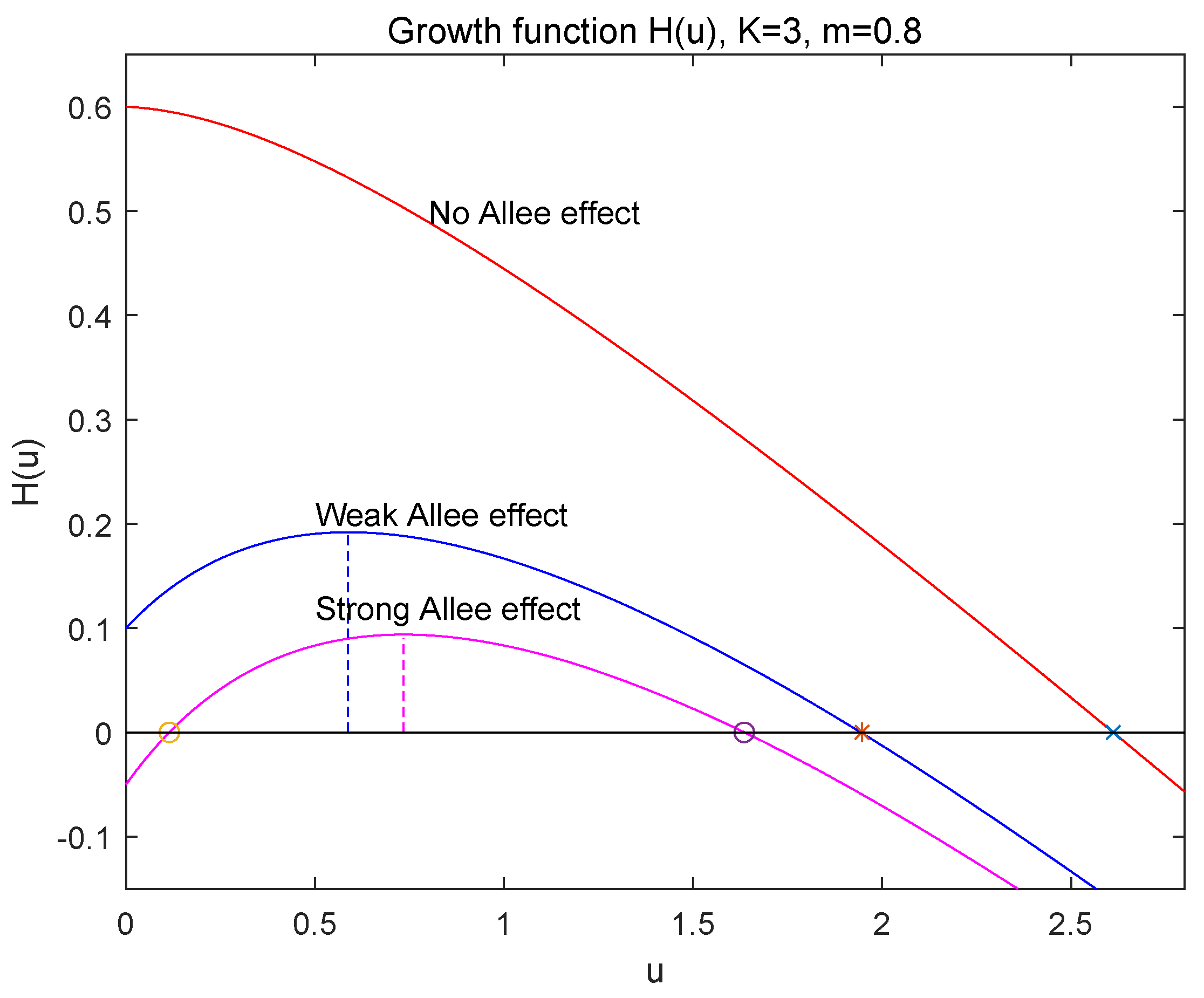
In order to have a complete understanding of the influence of the additive predation term on the dynamics of model (2), in this section we consider the dynamics of the single population model (1). Let
It is easy to see that has its local maximum at
and for while for . Since , we know that if the ratio of the attack rate a to the intrinsic growth rate r is large such that holds, then model (1) may admit an Allee effect (see [1]).
Clearly, is a trivial equilibrium of (1). The positive equilibria are the positive roots of , where
Let . If , i.e., , Equation (7) has two real roots and ():
By (7) and (8), it is easy to get the existence and stability of positive equilibria of model (1) (see [1]). However, to better understand the influences of the additive predation term on the dynamics of (1), we prefer the following analysis.
First, we show the following two cases in which the species tend to extinction.
- (i)
- (ii)
- If , i.e., , then the species u and hence v will be extinct since for all .
So, in what follows, the above two cases will not be discussed.
Now we consider the other cases as follows.
- (a)
- Assume .
- If , which implies that , then , has two positive roots and , which are given by (8) and satisfy that and since (see Figure 1). Thus, is locally asymptotically stable, is unstable and is locally asymptotically stable. So, in this case, the strong Allee effect appears in population growth of (1) and is the Allee threshold. The species u will be extinct when the initial population size is below , i.e., , and persistent when .
- (b)
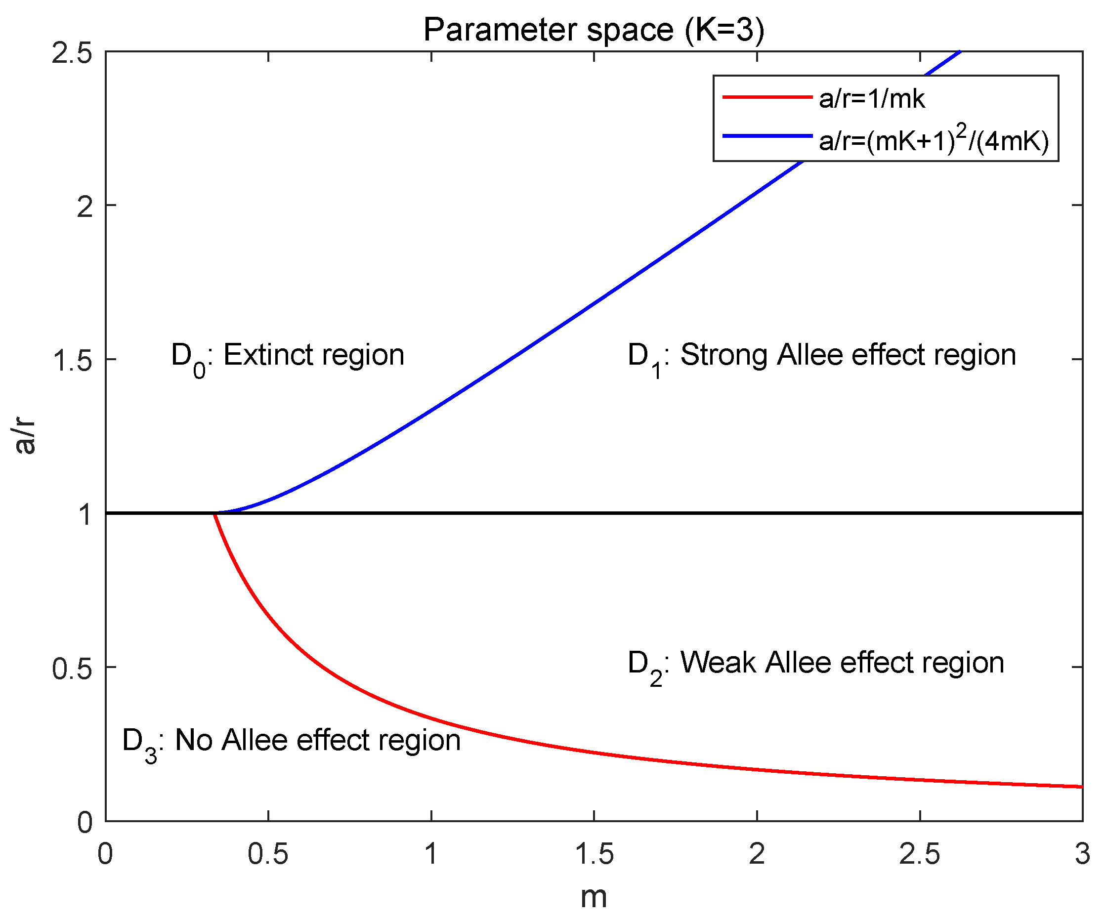
Based on the above arguments, we define the parameter space and (see Figure 2):
- Extinct region: ,
- Strong Allee effect region: ,
- Weak Allee effect region: ,
- No Allee effect region: .
From the above analysis, the ratio of the attack rate a of the additive predation to the intrinsic growth rate r of the species plays a key role in the dynamics of model (1). The large ratio goes against the population survival.
Define
It is easy to see that
If u is a positive root of , then and . Thus, we have the following result, which will be used in the later arguments.
Lemma 1.
If and exist, then and .
In the later arguments, we always assume that ; that is, model (2) has a strong Allee effect, weak Allee effect or no Allee effect.
3. Dynamics of the Predator–Prey Model
3.1. Positivity and Boundedness
Theorem 1.
1. Both X and are the positively invariant sets of model (2).
Proof.
1. For and , we have , which implies that both and are invariant manifolds. Due to the continuity of model (2), we can conclude that (2) is positively invariant in X and .
2. From the arguments on the function in Section 2, for the strong or weak Allee effect case, or no Allee effect case, has a positive root such that for . Thus, by the positivity of (2), the first equation of (2) yields and . This implies . Then, for any , there exists such that for , . Let , then , . It follows that . Hence, model (2) is uniformly ultimately bounded in X. □
Remark 1.
Theorem 1 indicates that the population size of prey u ultimately cannot go beyond . That is to say, is the largest size that the prey u may eventually achieve.
3.2. Equilibria
From the arguments on the single model (1) in Section 2, model (2) always has the trivial boundary equilibrium , and has at most two semi-trivial equilibria and , where and are the positive roots of , defined as (8).
When , model (2) has the unique positive equilibrium , where
3.3. Dynamics of the Strong Allee Effect Case
In this subsection, we consider the dynamics of model (2) in the strong Allee effect case. First we show the existence and local stability of equilibria, and that the Hopf bifurcation occurred at the positive equilibrium . Then we prove the non-existence of limit cycle when , and discuss the extinction of (2). In addition, based on these arguments and numerical simulations, the dynamics of global features of (2) are presented.
The linearized matrix of (2) with respect to any of its equilibria can be expressed as
where
(11) gives the characteristic equation
Lemma 2.
, if it exists, is locally asymptotically stable when , and unstable when .
Proof.
At , the characteristic Equation (12) becomes
So the result is clear. □
Theorem 2.
- 1.
- 2.
- is a stable node.
- 3.
- If , is a saddle with its unstable manifold along the u axis and its stable manifold (denoted by ) entering from the interior of ; if , is an unstable node.
- 4.
- If , is saddle with its stable manifold along the u axis and its unstable manifold (denoted by ) entering the interior of ; if , is a stable node.
- 5.
- The positive equilibrium is locally asymptotically stable when and unstable when . When , model (2) undergoes the Hopf bifurcation at .
Proof.
From the arguments of the function in Section 2, in the strong Allee effect case, model (2) has three boundary equilibria , and . Since when , by (10), we know that the positive equilibrium exists if and only if .
At , (12) has the eigenvalues and . Thus, is a stable node since .
At the semi-trivial boundary equilibrium , the characteristic Equation (12) becomes
which gives two eigenvalues and , where are defined as (9). At , by Lemma 1, and hence the third part of the result holds. At , , so the fourth part also holds.
In the strong Allee effect case, from the arguments on the function in Section 2, for and for . Then, by Lemma 2, the positive equilibrium is locally asymptotically stable when and unstable when .
When , the characteristic Equation (13) has a pair of imaginary eigenvalues . Then, the Hopf bifurcation occurs at . In fact, by taking as bifurcation parameter, we have since . Notice that and since is concave. Thus, , which implies from the Poincaré–Andronov–Hopf Bifurcation Theorem [39] that model (2) undergoes a Hopf bifurcation at when . □
Remark 2.
Theorem 3.
Proof.
When , according to Theorem 2, is a stable node, both and are saddle, the positive equilibrium exists and is unstable. Assume that model (2) has a periodic orbit with period T. Then, by integrating the equations of (2) on , we have
Denote the right-hand sides of (2) as and , respectively. By (15), we get the integral of divergence of (2):
Let and . We consider the positive half-trajectory passing the point . By examining the direction of the vector field in model (2), must pass the v-nullcline above the u-nullcline and enter the region .
If does not enter the region , then must intersect the line at some point . Thus, we can construct a region with the vertices and as follows: Between and , the boundary of is the orbit , and all other parts of the boundary of are the line segments connecting . It is easy to see that is negatively invariant. Since is the unique equilibrium point in the first quadrant, any periodic orbit, if it exists, must encircle it and lie wholly in the region . Assume is a T-periodic orbit in . Then and hence . Thus, from (16). This implies that the periodic orbit is unstable. However, it is impossible since is unstable.
Assume that enters the region . After that, if always stays on the left of the line , then its -limit set must be a periodic orbit. From (16) the periodic orbit is unstable. However, this is also impossible since is unstable. If intersects the line at some point , then we can construct the region as follows: Its boundaries are composed of the segment of orbit from to and the straight line segment between and . Clearly, is negatively invariant. Similar to the above arguments, model (2) has no periodic orbit. □
Remark 3.
From Theorems 2 and 3, we can conclude that when , the forward and subcritical Hopf bifurcation occurs at the positive equilibrium (see Figure 3). That is, as increases from , model (2) has an unstable limit cycle bifurcating from the positive equilibrium . When , both and are saddle, and model (2) may have a heteroclinic orbit connecting to (see Figure 3e).
Now we show the extinction of model (2).
Theorem 4.
Proof.
Let . By from Theorem 1, we have that for sufficiently small satisfying , there exists such that for all , . Then by the second equation of (2), we have that . It follows that .
If , then according to Theorem 2, model (2) only has three boundary equilibria , and , where is a stable node, is an unstable node and is a saddle. Theorem 1 implies that (2) has a compact global attractor. Thus, from an application of the Poincaré–Bendixson theorem [40] we conclude that for any solution of (2) initiated from the interior of ; that is, is globally asymptotically stable.
Remark 4.
Theorem 4 indicates the following biological implications.
- i.
- The first part is about the extinction of predator species due to the large ratio of the death rate d to the conversion rate β of predator species.
- ii.
- The second part is about the extinction due to the strong Allee effect of the prey population driven by the additive predation . implies that the invasion or reproduction of the predator v is excessive while the reproduction of the prey u is not fast enough to sustain its own population. Thus, the excessive invasion or reproduction of the predator v drives the population of the prey u to below its Allee threshold and eventually to zero, which consequently drives the predator population to extinction.
- iii.
- The third statement indicates that when the population density of the prey is below its Allee threshold , all species will be extinct.
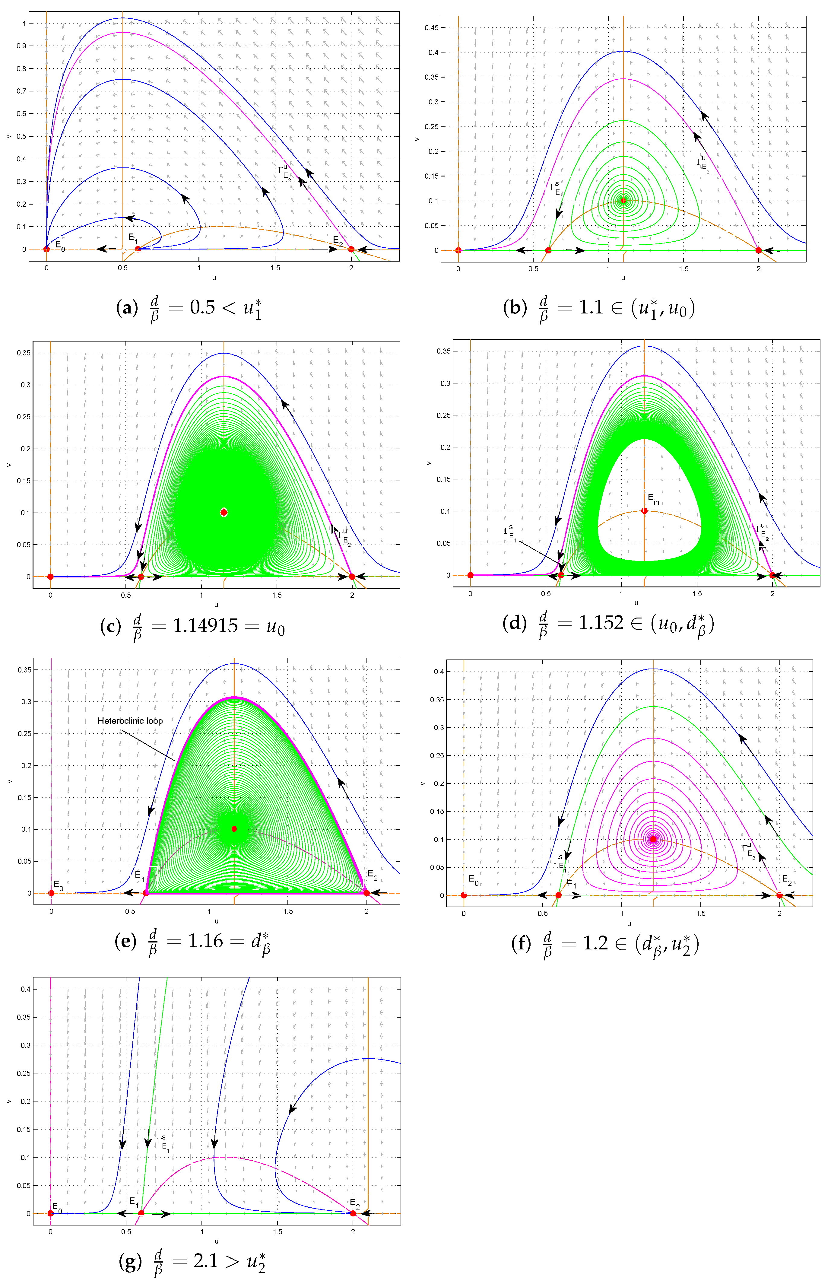
Now, let and be fixed such that model (2) exhibits the strong Allee effect. By the previous discussion and numerical simulations, as varies, we show the dynamics of global features of (2) (see Figure 3).
- (i)
- . is a stable node, is an unstable node, is a saddle. There is no interior equilibrium. All trajectories in the interior of converge to ; two species will be extinct (see Figure 3a).
- (ii)
- . becomes a saddle and an unstable interior equilibrium appears. Around , there is no limit cycle. Except for the stable manifold of , all trajectories converge to (see Figure 3b).
- (iii)
- . A forward subcritical Hopf bifurcation occurs (see Figure 3c).
- (iv)
- . Both and are saddle and the interior equilibrium become locally asymptotically stable. There exists a threshold value such that
- (a)
- when , there exists an unstable limit cycle surrounding . Outside the limit cycle, two species cannot coexist, while inside the limit cycle trajectories converge towards the stable interior equilibrium (see Figure 3d);
- (b)
- when , the limit cycle disappears and a heteroclinic loop connecting to appears. Outside the heteroclinic loop, trajectories converge to , and two species will be extinct, while inside the heteroclinic loop trajectories converge towards the heteroclinic loop, and two species coexist (see Figure 3e);
- (c)
- when , the heteroclinic orbit is broken. Above the stable manifold of , trajectories converge to , and two species will be extinct, while below , trajectories converge towards the stable interior equilibrium , and two species coexist (see Figure 3f).
- (v)
- . There is a transcritical bifurcation at . When increasing the value of from , becomes a stable node and the interior equilibrium disappears. This leads to the predator free dynamics with as attractors (see Figure 3g).
3.4. Dynamics of the Weak Allee Effect Case
In this subsection, we consider the dynamics of model (2) in the weak Allee effect case, including the existence of equilibria, the local dynamics and the global feature of (2).
First, we show the existence and local stability of equilibria.
Theorem 5.
- 1.
- 2.
- is always an unstable saddle.
- 3.
- is a stable node when and an unstable saddle when .
- 4.
- The positive equilibrium is locally asymptotically stable when and unstable when . When , system (2) undergoes the Hopf bifurcation at .
Proof.
In the weak Allee effect case, by the property of shown in Section 2, model (2) has two boundary equilibria and . The positive equilibrium exists if and only if .
At , (12) has the eigenvalues and . Thus, is a saddle.
At , the characteristic Equation (14) has two eigenvalues and . By Lemma 1, . Thus, is a stable node when and a saddle when .
In the weak Allee effect case, from the property of shown in Section 2, for and for . Then, by Lemma 2, the positive equilibrium is locally asymptotically stable when and unstable when .
When , similar to the arguments of the strong Allee effect case, the Hopf bifurcation occurs at . □
Theorem 6.
Proof.
1. In the weak Allee effect case and , by Theorem 5, model (2) has two boundary equilibria and , in which is a saddle and is a stable node, and has no positive equilibrium. Thus, from an application of Poincaré–Bendixson theorem [40] we conclude that is globally asymptotically stable.
2. When , both and are saddle, and exists and is locally asymptotically stable by Theorem 5. The stable and unstable manifolds of are along the v-axis and u-axis, respectively. The stable manifold of is along the u-axis and its unstable manifold enters the interior of . If (2) has no limit cycle, then from Poincaré–Bendixson theorem [40] we can conclude that is globally asymptotically stable. On the contrary, we assume that model (2) has a periodic orbit with period T. Then, (16) holds.
Let and . We consider the negative half-trajectory passing the point . By examining the direction of vector field in model (2), must pass the v-nullcline above the u-nullcline and enter the region .
If does not enter the region , then must intersect the line at some point . Thus, we can construct a region with the vertices and as follows: Between and , the boundary of is the orbit , and all other parts of the boundary of are the line segments connecting . It is easy to see that is positively invariant. Since is the unique equilibrium point in the first quadrant, any periodic orbit, if it exists, must encircle it and lie wholly in the region . Assume is a T-periodic orbit in . Then and hence . Thus, from (16). This implies that the periodic orbit is stable. However, it is impossible since is locally asymptotically stable.
Assume that enters the region . After that, if always stays on the right of the line , then its -limit set must be a periodic orbit. From (16) the periodic orbit is stable. However, this is also impossible since is locally asymptotically stable. If intersects the line at some point , then we can construct the region as follows: Its boundaries are composed of the segment of orbit from to and the straight line segment between and . Clearly, is positively invariant. Similar to the above arguments, model (2) has no periodic orbit.
3. Let . By Theorem 5, both and are saddle, and exists and is unstable. Define , where is a positive constant to be determined. Let be the region bounded by the lines , , and . When , since and , we know that all orbits of model (2) must ultimately pass through the line from right to left.
Along the line , we have
Thus, we can choose sufficiently large such that for . This implies that the orbit that meets the line must pass through it from the upper right to the lower left. Therefore, is a bounded positive invariant set of (2). By Poincaré–Bendixson theorem [40], model (2) has a stable limit cycle surrounding . □
3.5. Dynamics of No Allee Effect Case
In this subsection, we consider the dynamics of model (2) in the no Allee effect case. First, similar to the case of weak Allee effect, we have the following result on the existence and local stability of equilibria.
Theorem 7.
- 1.
- 2.
- is always an unstable saddle.
- 3.
- is a stable node when and an unstable saddle when .
- 4.
- If the positive equilibrium exists, it is locally asymptotically stable.
Now we state the global dynamics behavior of model (2).
Theorem 8.
- 1.
- If , then is globally asymptotically stable.
- 2.
- If , then is globally asymptotically stable.
Proof.
Similar to the proof of the first part of Theorem 4, one can prove the global stability of .
Let , then exist. Assume model (2) has a limit cycle, then, by (see Theorem 1), it must lie on the left of the line . From the arguments on the function in Section 2, for . Thus, from (16), from (16). This implies that the limit cycle is stable. However, it is impossible since is locally asymptotically stable. Therefore, is globally asymptotically stable. □
Remark 6.
Similar to Theorem 6, Theorem 8 also indicates the following biological implications.
- i.
- If the ratio is large such that , then the predator species u will be extinct.
- ii.
- If , both species u and v can coexist.
3.6. Summary of the Dynamics of Model
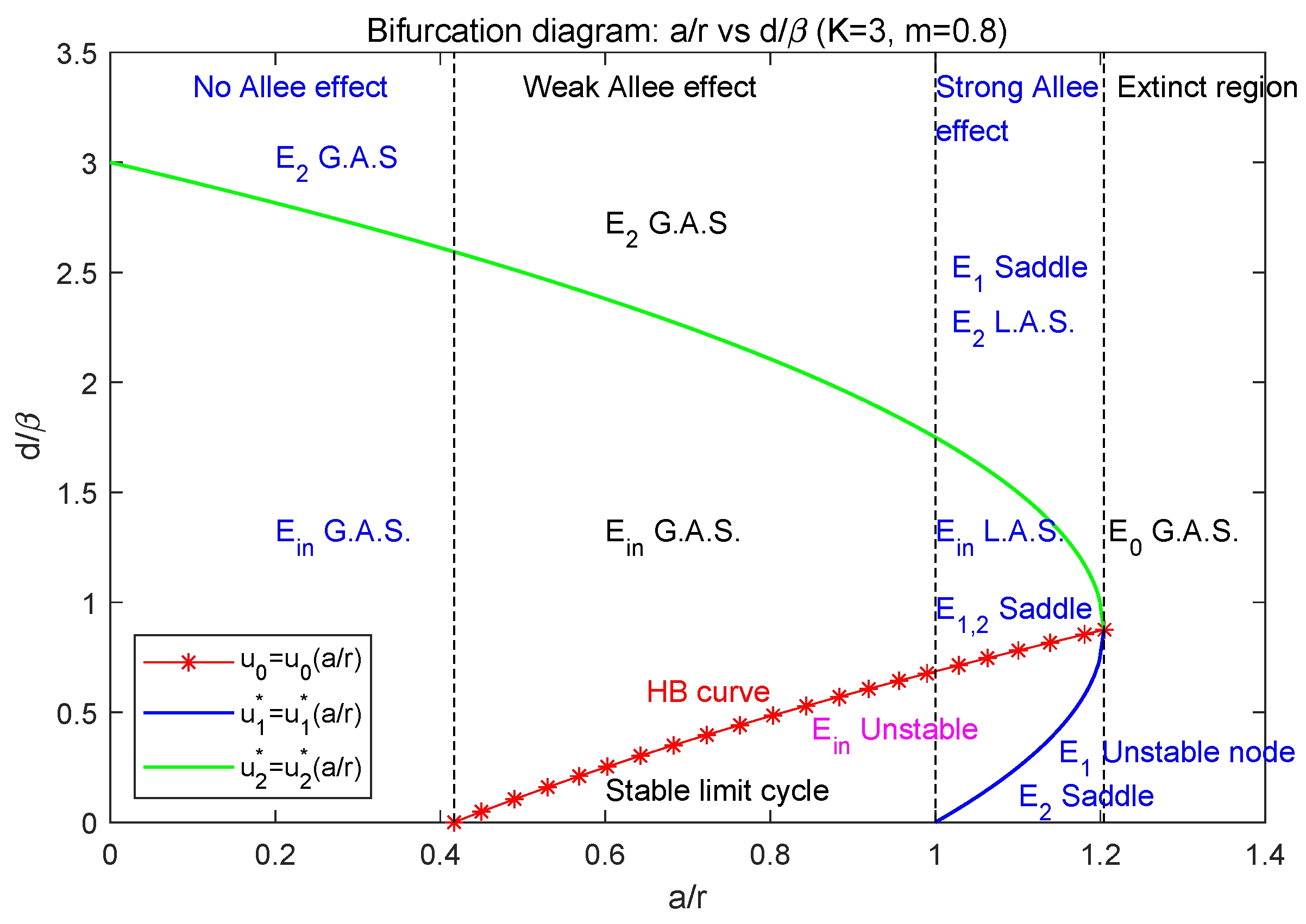
From (8) and (6), we know that with respect to , and increase while decreases, and when , i.e., . In the plane, the main dynamics of model (2) can be concluded as in Figure 5, in which , the green curve denotes , the blue curve denotes , and the red-star curve denotes the Hopf bifurcation curve .
- (1)
- When , the parameter lies in the extinct region, i.e., ; model (2) only has the extinction equilibrium which is globally asymptotically stable. In this case, both the predator and prey species will be extinct.
- (2)
- When , model (2) admits the strong Allee effect. In this case, model (2) has three boundary equilibria , where is a stable node (see Section 3.3).
- (2.1)
- (2.2)
- Below the blue curve (i.e., ), is a saddle, is an unstable node, and is globally asymptotically stable. So, two species will be extinct (see Figure 3a).
- (2.3)
- Between the blue and green curves (i.e., ), the interior equilibrium exists, and both and are saddle. Between the red and green curve (i.e., ), is locally asymptotically stable; between the blue and red curve (i.e., ), it is unstable; along the red curve (i.e., ), Hopf bifurcation occurs. The two species may coexist but it depends on their initial population sizes. In this case, model (2) may have the heteroclinic loop connecting and (see Figure 3b–f).
- (3)
- When , model (2) has weak Allee effect. In this case, model (2) has two boundary equilibria , where is a saddle (see Section 3.4).
- (3.1)
- (3.2)
- Below the green curve (i.e., ), the interior equilibrium exists, is a saddle. Between the red and green curve (i.e., ), is globally asymptotically stable; below the red curve (i.e., ), model (2) has a stable limit cycle surrounding ; along the red curve (i.e., ), Hopf bifurcation occurs. So, in this case, two species can coexist (see Figure 4a–c).
- (4)
- When , model (2) has no Allee effect. In this case, model (2) has two boundary equilibria , where is a saddle (see Section 3.5).
- (4.1)
- Above the green curve (i.e., ), model (2) has no positive equilibrium; is globally asymptotically stable; that is, the predator will be extinct while the prey is permanent.
- (4.2)
- Below the blue curve (i.e., ), the interior equilibrium exists and is globally asymptotically stable. So, in this case, two species can coexist.
4. The Influence of Delay
In this section, we consider the delayed model (3) and study the Hopf bifurcations caused by the delay.
4.1. Stability and Hopf Bifurcation Induced by Delay
The characteristic equation is given by , i.e.,
At , (17) becomes , where . Thus, for all , is locally asymptotically stable if , and unstable if .
At the semi-trivial boundary equilibrium , is given by (8), (17) becomes
which gives an eigenvalue . Thus, if and only if . The other eigenvalues are determined by
At , since by Lemma 1, we know that (19) has roots with positive real parts for each by Theorem 4.7 from Smith [33], which implies that is always unstable for all .
At , by Lemma 1, then by Theorem 4.7 from Smith [33] there exists a , which is given by
such that the real parts of all roots of (19) are negative for , and (19) has roots with positive real parts for each . Therefore, we can conclude that when , is locally asymptotically stable for , and unstable for ; when , is unstable for all .
Let . Now we show that when , model (3) undergoes the Hopf bifurcation at . As varies, if the stability of switches at , then the characteristic Equation (18), i.e., the Equation (19), must have a pair of pure conjugate imaginary roots when (see [33,34]). Let be a root of (18) (i.e., (19)), then we have and . Thus, one can get the unique critical delay and the value . By differentiating (18) with respect to , we have
At and , and ; thus, we get
It follows
This implies that, with increasing , all the roots of (19) (and hence (18)) that cross the imaginary axis at cross from left to right whenever ; therefore, the stability of boundary equilibrium undergoes a switch from stable to unstable, and the Hopf bifurcation occurs at .
Conclusively, we have the following result.
Theorem 9.
- 1.
- For all , is locally asymptotically stable if , and unstable if .
- 2.
- If exists, it is unstable for all .
- 3.
- If exists, then (i) when , there exists a such that is locally asymptotically stable for , unstable for , and undergoes Hopf bifurcation at ; (ii) when , is unstable for all .
At the positive equilibrium , where , (17) becomes
Denote . It is clear that . For convenience, in what follows we write and as and , respectively.
Let be a root of ; then, we have
which follows
It is easy to see that (23) has positive roots if and only if
Notice that . Therefore,
Let , i.e., . Substituting into (22), we get
Let . Since
we get ; that is, . Thus, we obtain the following two sets of values of for which (21) has imaginary roots:
We need to determine the sign of the derivative of at the points where is purely imaginary. From (21), we have
Then we have
Thus,
Since , we get
This implies that, with increasing , all the roots of (21) that cross the imaginary axis at cross from left to right whenever , and cross at from right to left for .
By Lemma 2, as , is locally asymptotically stable when (i.e., ). Then it must follow that . Observe that
Then there exists a positive integer p such that
It follows that model (3) is locally asymptotically stable at for , unstable for , and undergoes Hopf-bifurcation at and .
From the above analysis, we have the following result.
4.2. Direction and the Stability of Hopf-Bifurcating Periodic Solutions
In this subsection, we use the normal form method and the center manifold theory introduced by Hassard et al. [36] to analyze the properties of Hopf bifurcation around and , respectively, including the direction of Hopf bifurcation, and the stability and period of the Hopf-bifurcating periodic solutions. These properties are determined by the following three quantities:
where is the critical time delay such that the characteristic equation has the pure conjugate imaginary roots, and
In the three quantities of (26), determines the direction of Hopf bifurcation, determines the stability of Hopf-bifurcating periodic solutions, and T determines the period of Hopf-bifurcating periodic solutions. More precisely (see [35]),
- (1)
- If (resp. ), then the Hopf bifurcation is supercritical (resp. subcritical).
- (2)
- If (resp. ), then the periodic solution is orbitally asymptotically stable (resp. unstable).
- (3)
- If (resp. ), then the period of bifurcating periodic solutions increases (resp. decreases) as the bifurcation parameter (delay time ) keeps away from the critical value.
In order to get the three important quantities of Hopf bifurcation, it is key to compute the coefficients and . In what follows, we present the computation of these coefficients at the equilibria and , respectively. The calculation process is similar to that in many references (see, e.g., [41,42,43,44,45]).
4.2.1. At the Positive Equilibrium
From Theorem 10, at the positive equilibrium , when , the characteristic Equation (21) has a pair of conjugate pure imaginary roots given by (24), and model (3) undergoes the Hopf bifurcation. Let be a critical delay value in the set and be the corresponding conjugate pure imaginary roots of (21). In what follows, we determine the three quantities given in (26) at .
Let , , , . Denote . Define , as follows
where
Then model (3) can be written as the following functional differential equation
By the Riesz representation theorem, there is a matrix function of bounded variation for , such that . We choose , where
For , define the operators
and
Then (28) is equivalent to
where for .
For , define the operator
and a bilinear inner product
where . Then and are adjoint operators. According to the previous calculation, we know that are the eigenvalues of , so are also the eigenvalues of .
Suppose that and are the eigenvectors of and corresponding to and , respectively. Then and . With the definition (29) of , we get
and then we have , i.e., .
Thus, .
Now, by the ideas in Hassard et al. [36], we calculate the coordinates to describe the center manifold at . For this purpose, let be the solution of Equation (28) when , and define
on the center manifold , we have
where , Z and are the local coordinates of in the direction of and .
Note that W is real if and only if is real. Here we only consider real solutions. For the solution of Equation (28), when , we have
where .
From (32), we have . Combined with the definitions of W and , the following expressions can be obtained
By the definitions of and , can be rewritten as
So, we get the following coefficients:
From (34), we know that for ,
By comparing the coefficients, we get
Combining the definition of A, we obtain
From (35), we get
Since , we have
By these two equations, we get
where
Thus, by (33), (36) and (39), the coefficients and can be computed and hence the three quantities (26) of Hopf bifurcation at can be determined.
For example, we take the following parameters:
This set of parameters implies that model (3) has a strong Allee effect since . One can get the positive equilibrium , which is locally asymptotically stable for model (2) without delay since by Lemma 2. For the delayed model (3), by (25), the critical delay values are computed as follows:
So, we have
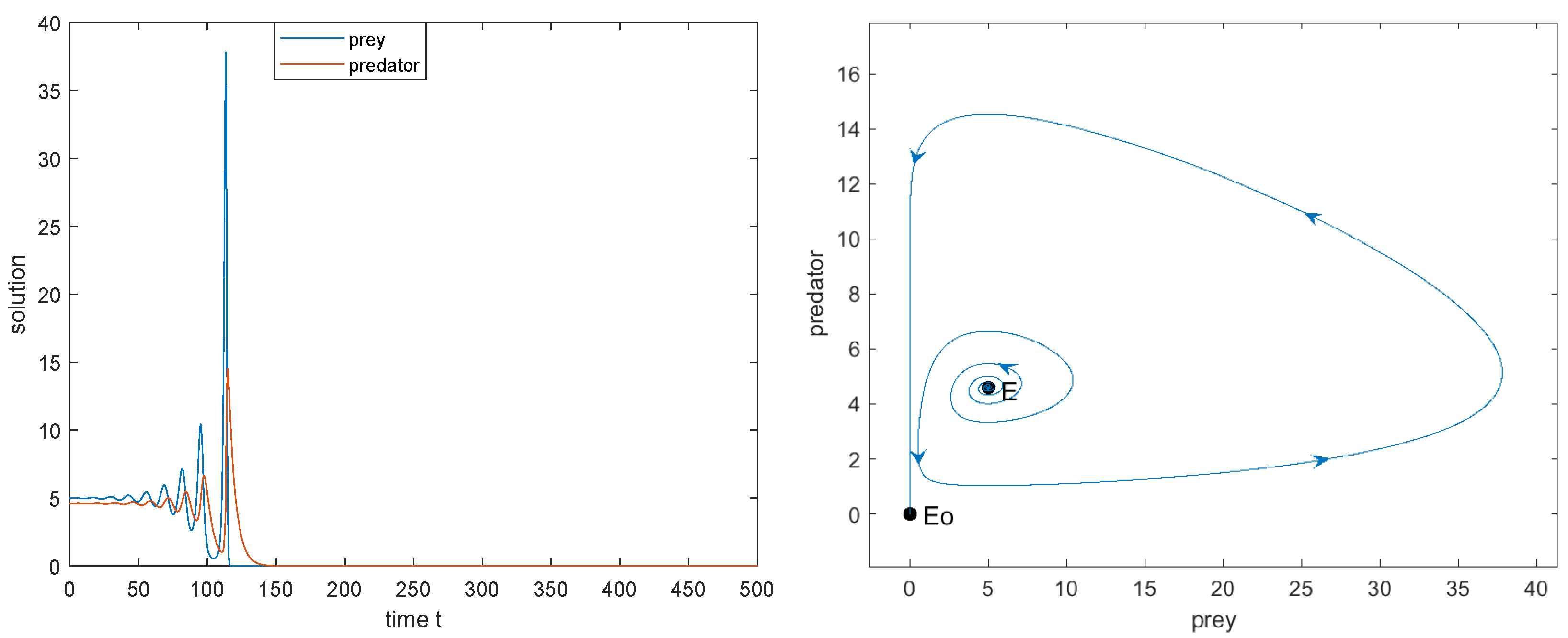
From Theorem 10, we know that as is increasing, the stability of switches twice and is locally asymptotically stable for and unstable for , while model (3) undergoes the Hopf bifurcation at when takes and , respectively; see Figure 6, Figure 7, Figure 8, Figure 9, Figure 10, Figure 11 and Figure 12, in which the dynamics of (3) are presented as is increasing.
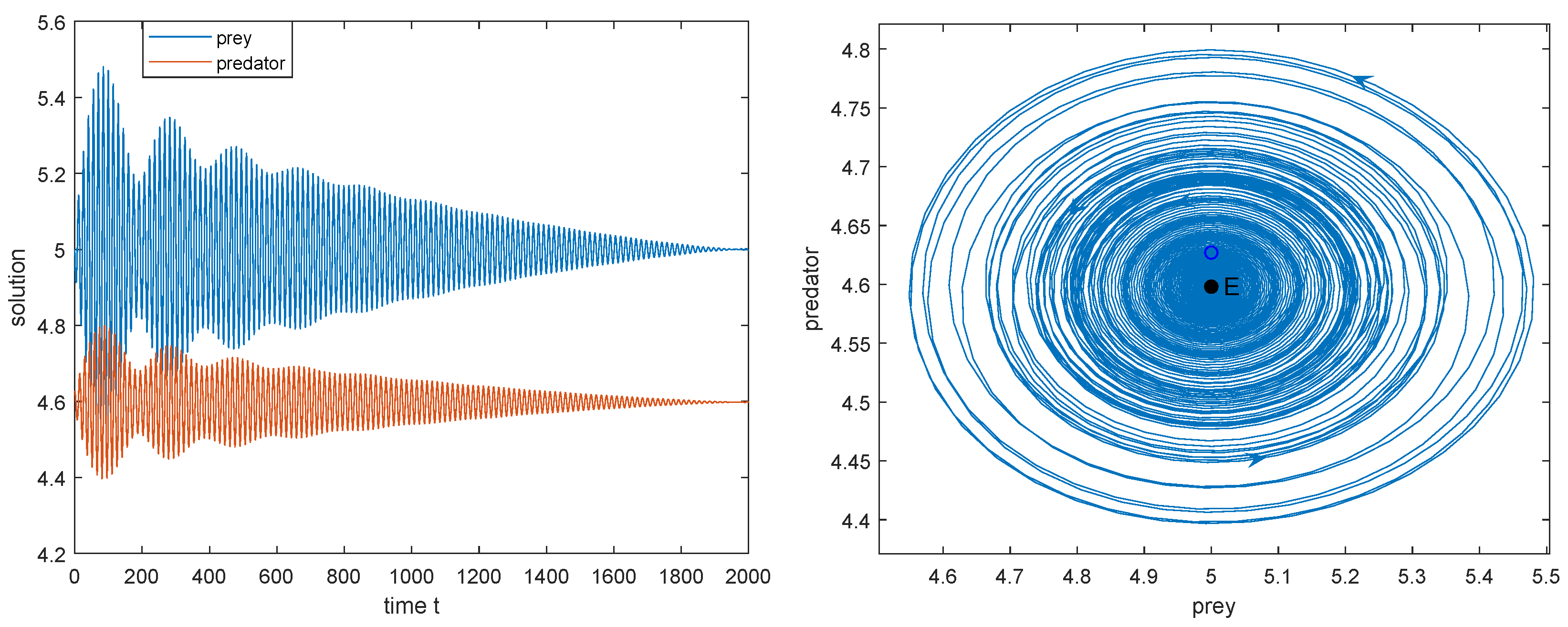
1. Taking , then is locally asymptotically stable (see Figure 6), which implies that both the predator and prey can coexist.
2. Taking as the Hopf bifurcation value , we have the three quantities (26) of Hopf bifurcation: . Thus, the Hopf bifurcation is subcritical since and the periodic Hopf orbit is unstable since (see Figure 7).
3. Taking , is unstable (see Figure 8).
4. Choosing as the Hopf bifurcation value , we have , , which implies that the Hopf bifurcation is subcritical and the periodic Hopf orbit is asymptotically stable (see Figure 9).
5. Taking , is locally asymptotically stable (see Figure 10).
6. Choosing , we have ; then the Hopf bifurcation is supercritical since and the bifurcating periodic solution is orbitally asymptotically stable since (see Figure 11).
7. Taking , is unstable (see Figure 12).
It can be observed from Figure 6, Figure 7, Figure 8, Figure 9, Figure 10, Figure 11 and Figure 12 that the delay has a large influence on the long-term community stability, showing the stability changes for small values of , which represents the density dependent feedback time introduced in the logistic growth. The occurrence of Hopf bifurcation at implies the emergence of periodic solutions. From the biological viewpoint, if the periodic solution bifurcating from is stable, then the predator and prey species may coexist in an oscillatory mode.
4.2.2. At the Semi-Trivial Equilibrium
From Theorem 9, when , model (3) undergoes the Hopf bifurcation at the semi-trivial equilibrium for , and are the corresponding conjugate pure imaginary roots of the characteristic Equation (18). Similar to the discussion on , the computation of coefficients and at are presented as follows.
where
Thus, the three quantities (26) of Hopf bifurcation at also can be determined.
For example, we take
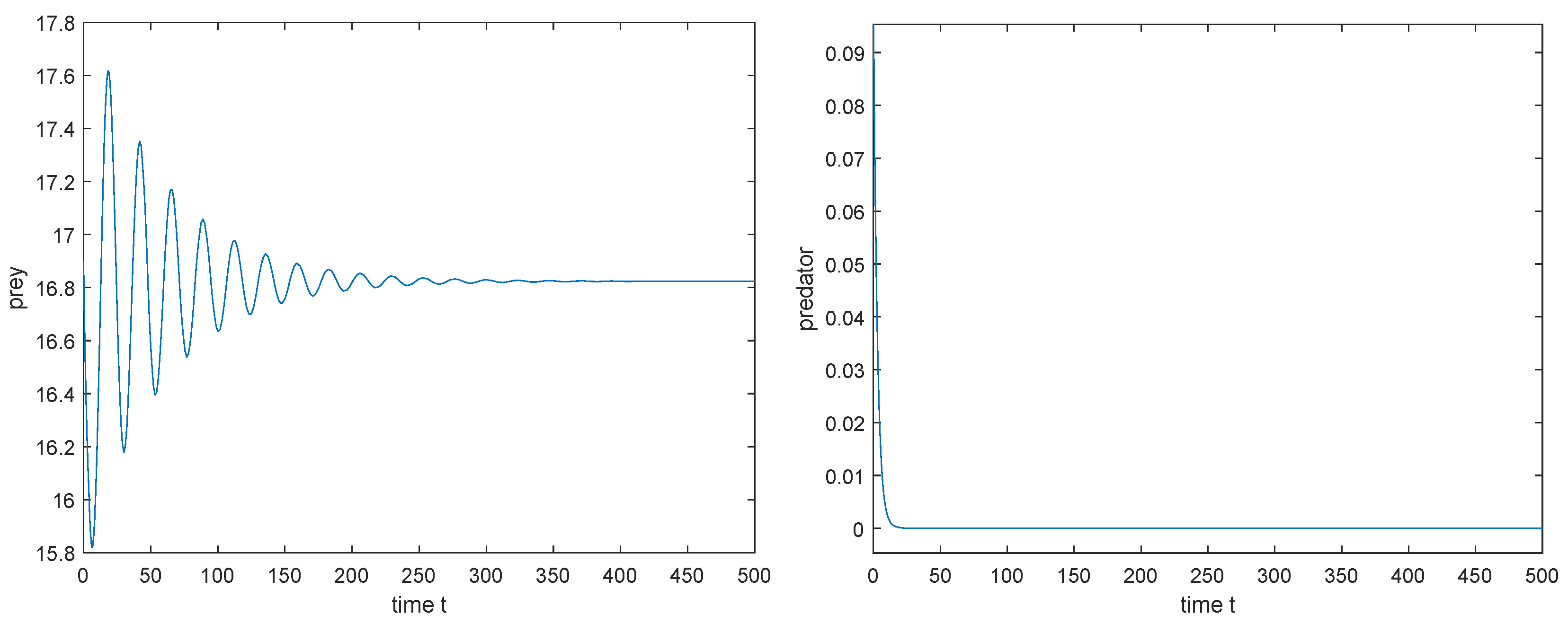
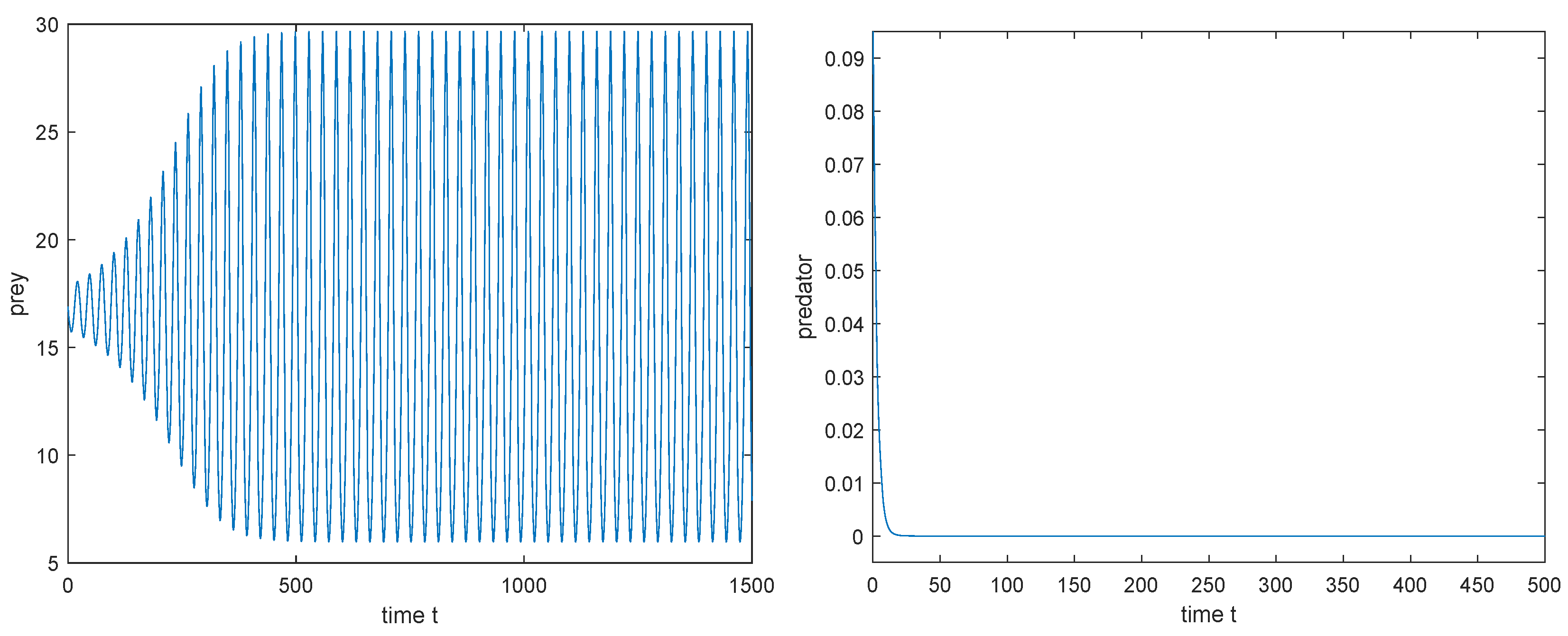
Then, , , . From Theorem 9, we know that is locally asymptotically stable when and unstable when , and the Hopf bifurcation occurs at , which also can be seen from Figure 13, Figure 14 and Figure 15.
1. Taking , then is locally asymptotically stable (see Figure 13), which implies that the prey can survive and the predator will be extinct.
2. Taking as the Hopf bifurcation value , we have the values defined by (26): . Then the Hopf bifurcation is supercritical since and the periodic solution bifurcating from is orbitally asymptotically stable since (see Figure 14).
3. Taking , is unstable (see Figure 15), and model (3) has a periodic boundary solution bifurcating from the Hopf bifurcation.
From Figure 13, Figure 14 and Figure 15, it was observed that the delay also has a large influence on the stability of boundary equilibrium . As the delay increases, goes from stable to unstable. The occurrence of Hopf bifurcation at implies the emergence of boundary periodic solution . If the boundary periodic solution bifurcating from the steady state is stable, then the prey species may survive in an oscillatory mode while the predator will be extinct.
5. Conclusions
In this paper, we proposed a predator–prey model (2), in which the prey’s growth is affected by the additive predation of all potential predators. Due to the additive predation term , model (2) may exhibit the cases of strong Allee effect, weak Allee effect and no Allee effect (see Section 2 and Figure 2). In each case, the dynamics of (2) are investigated. From our analysis, the ratio of the attack rate a of other potential predators to the intrinsic growth rate r of prey species u, and the ratio of the death rate d to the conversion rate of predator species, play a key role in the dynamics of model (2). The main dynamics of model (2) was described conclusively in a bifurcation diagram with respect to (see Figure 5), and the biological explanations of the obtained results were presented (see Remarks 4–6 and Section 3.6). From Theorems 6 and 8, the coexistence of predator and prey can be achieved by controlling the ratio such that model (2) has weak Allee effect or no Allee effect, and the ratio such that it is below the largest size that the prey u may eventually achieve.
When the additive predation is not involved in model (2), then (2) is the well-known Lotka–Volterra type model
which has been well studied (see, e.g., [37,38]). If the positive equilibrium of (40) exists, then it must be globally asymptotically stable, which implies that both the species coexist.
- (i)
- Due to the additive predation term , model (2) may have the Allee effect;
- (ii)
- The dynamics of the Lotka–Volterra type model (40) only have the similar dynamic structure of (2) in the case of no Allee effect (see Section 3.4), but have no dynamics of the strong and weak Allee effect cases;
- (iii)
- Model (2) may have oscillatory behavior;
- (iv)
- The strong Allee effect increases the extinction risk of the prey and predator species. The initial populations of the prey and predator play an important role in the persistence of (2). Not only the low initial prey density, but also the high initial predator density which causes the over-exploitation of the prey, will lead to the extinction of all species. For a set of parameter values, both community extinction, coexistence, and population oscillations may be the result of different initial conditions;
- (v)
In Section 4, the stability and Hopf bifurcation of model (3) with the density dependent feedback time delay in prey were considered. By the normal form method and center manifold theory, the explicit formulas are presented to determine the direction of Hopf bifurcation and the stability and period of Hopf-bifurcating periodic solutions. In addition, some numerical simulations are given to illustrate the theoretical results. Theoretical analysis and numerical simulation indicate that the delay may destabilize model (3), and cause the Hopf bifurcation not only at the interior equilibrium but also at the boundary equilibrium (see Theorems 9 and 10). Biologically, the occurrence of Hopf bifurcation at implies that both the predator and prey species may coexist in a mode of periodic oscillation; at it implies that the prey species may survive in an oscillatory mode while the predator will be extinct.
Author Contributions
Conceptualization, X.Z. and D.B.; methodology, D.B.; formal analysis, X.Z. and D.B.; writing—original draft preparation, X.Z.; writing—review and editing, D.B.; supervision, D.B. All authors have read and agreed to the published version of the manuscript.
Funding
This research was funded by NSF and SCTPP of Guangdong Province of China (2021A1515010310, 2020A1414010106) and NKRDP of China (2020YFA0712500).
Institutional Review Board Statement
Not applicable.
Informed Consent Statement
Not applicable.
Data Availability Statement
Not applicable.
Conflicts of Interest
The authors declare no conflict of interest.
References
- Kang, Y.; Udiani, O. Dynamics of a single species evolutionary model with Allee effects. J. Math. Anal. Appl. 2014, 418, 492–515. [Google Scholar] [CrossRef]
- Dennis, B. Allee effect: Population growth, critical density, and chance of extinction. Nat. Resour. Model. 1989, 3, 481–538. [Google Scholar] [CrossRef]
- Dercole, F.; Ferriére, R.; Rinaldi, S. Ecological bistability and evolutionary reversals under asymmetrical competition. Evolution 2002, 56, 1081–1090. [Google Scholar] [CrossRef] [Green Version]
- Allee, W.C. Animal Aggregations: A Study in General Sociology; University of Chicago Press: Chicago, IL, USA, 1931. [Google Scholar]
- Allee, W.C. Studies in animal aggregations: Mass protection against colloidal silver among goldfishes. J. Exp. Zool. 1932, 61, 185–207. [Google Scholar] [CrossRef]
- Kramer, A.M.; Dennis, B.; Liebhold, A.M.; Drake, J.M. The evidence for Allee effects. Popul. Ecol. 2009, 51, 341–354. [Google Scholar] [CrossRef]
- Berec, L.; Angulo, E.; Courchamp, F. Multiple Allee effects and population management. Trends Ecol. Evol. 2006, 22, 185–191. [Google Scholar] [CrossRef]
- Courchamp, F.; Berec, L.; Gascoigne, J. Allee Effects in Ecology and Conservation; Oxford University Press: Oxford, UK, 2008. [Google Scholar]
- Mooring, M.S.; Fitzpatrick, T.A.; Nishihira, T.T.; Reisig, D.D. Vigilance, predation risk, and the Allee effect in desert bighorn sheep. J. Wildl. Manag. 2004, 68, 519–532. [Google Scholar] [CrossRef]
- Rinella, D.J.; Wipfli, M.S.; Stricker, C.A.; Heintz, R.A.; Rinella, M.J. Pacific Salmon (Oncorhynchus sp.) runs and consumer fitness: Growth and energy storage in stream-dwelling salmonids increase with salmon spawner density. Can. J. Fish. Aquat. Sci. 2012, 69, 73–84. [Google Scholar] [CrossRef]
- Stephens, P.A.; Sutherland, W.J. Consequences of the Allee effect for behaviour, ecology and conservation. Trends Ecol. Evol. 1999, 14, 401–405. [Google Scholar] [CrossRef]
- Stephens, P.A.; Sutherland, W.J.; Freckleton, R.P. What is the Allee effect? Oikos 1999, 87, 185–190. [Google Scholar] [CrossRef] [Green Version]
- Wang, M.E.; Kot, M. Speeds of invasion in a model with strong or weak Allee effects. Math. Biosci. 2001, 171, 83–97. [Google Scholar] [CrossRef]
- Courchamp, F.; Clutton-Brock, T.; Grenfell, B. Inverse density dependence and the Allee effect. Trends Ecol. Evol. 1999, 14, 405–410. [Google Scholar] [CrossRef]
- Conway, E.D.; Smoller, J.A. Global analysis of a system of predator–prey equations. SIAM J. Appl. Math. 1986, 46, 630–642. [Google Scholar] [CrossRef]
- Wang, J.; Shi, J.; Wei, J. Predator–prey system with strong Allee effect in prey. J. Math. Biol. 2011, 62, 291–331. [Google Scholar] [CrossRef] [PubMed]
- Lewis, M.A.; Kareiva, P. Allee dynamics and the spread of invading organisms. Theor. Popul. Biol. 1993, 43, 141–158. [Google Scholar] [CrossRef]
- Amarasekare, P. Allee effects in metapopulation dynamics. Am. Nat. 1998, 152, 298–302. [Google Scholar] [CrossRef]
- Zhou, S.; Liu, Y.; Wang, G. The stability of predator–prey systems subject to the Allee effects. Theor. Popul. Bio. 2005, 67, 23–31. [Google Scholar] [CrossRef]
- Gascoigne, J.C.; Lipcius, R.N. Allee effects driven by predation. J. Appl. Ecol. 2004, 41, 801–810. [Google Scholar] [CrossRef]
- Wilson, E.O.; Bossert, W.H. A Primer of Population Biology; Sinauer Assiates, Inc.: Sunderland, UK, 1971. [Google Scholar]
- Boukal, D.S.; Berec, L. Single-species models and the Allee effect: Extinction boundaries, sex ratios and mate encounters. J. Theoret. Biol. 2002, 218, 375–394. [Google Scholar] [CrossRef]
- Bai, D.; Kang, Y.; Ruan, S.; Wang, L. Dynamics of an intraguild predation food web model with strong Allee effect in the basal prey. Nonlinear Anal. RWA 2021, 58, 103206. [Google Scholar] [CrossRef]
- Kostitzin, V.A. Sur la loi logistique et ses generalizations. Acta Biotheor. 1940, 5, 155–159. [Google Scholar] [CrossRef]
- Wang, W. Population dispersal and Allee effect. Ric. Mat. 2016, 65, 535–548. [Google Scholar] [CrossRef]
- Dennis, B. The Dynamics of Low Density Populations. Ph.D. Thesis, The Pennsylvania State University, State College, PA, USA, 1982. [Google Scholar]
- Jacobs, J. Cooperation, optimal density and low density thresholds: Yet another modification of the logistic model. Oecologia 1984, 64, 389–395. [Google Scholar] [CrossRef] [PubMed]
- Jiang, J.; Song, Y.; Yu, P. Delay-induced triple-zero bifurcation in a delayed Leslie-type predator–prey model with additive Allee effect. Int. J. Bifurc. Chaos 2016, 26, 1650117. [Google Scholar] [CrossRef]
- Aguirre, P.; González-Olivares, E.; Sáez, E. Two limit cycles in a Leslie-Gower predator–prey model with additive Allee effect. Nonlinear Anal. RWA 2009, 10, 1401–1416. [Google Scholar] [CrossRef]
- Aguirre, P.; González-Olivares, E.; Sáez, E. Three limit cycles in a Leslie-Gower predator–prey model with additive Allee effect. SIAM J. Appl. Math. 2009, 69, 1244–1269. [Google Scholar] [CrossRef]
- Terry, A.J. Predator–prey models with component Allee effect for predator reproduction. J. Math. Biol. 2015, 71, 1325–1352. [Google Scholar] [CrossRef]
- Cai, L.; Zhao, C.; Wang, W.; Wang, J. Dynamics of a Leslie-Gower predator–prey model with additive Allee effect. Appl. Math. Model. 2015, 39, 2092–2106. [Google Scholar] [CrossRef]
- Smith, H. An Introduction to Delay Differential Equations with Applications to the Life Sciences; Springer: New York, NY, USA, 2011. [Google Scholar]
- Kuang, Y. Delay Differential Equations: With Applications in Population Dynamics; Academic Press: New York, NY, USA, 1993. [Google Scholar]
- Wei, J.; Wang, H.; Jiang, W. Bifurcation Theory of Delay Differential Equations; Science Press: Beijing, China, 2012. (In Chinese) [Google Scholar]
- Hassard, B.D.; Kazarinoff, N.D.; Wan, Y.H. Theory and Applications of Hopf Bifurcation; Cambridge University Press: Cambridge, UK, 1981. [Google Scholar]
- Ma, Z. Mathematical Modeling and Research of Population Ecology; Anhui Education Press: Hefei, China, 1996. (In Chinese) [Google Scholar]
- Chen, L. Mathematical Ecological Models and Research Methods; Science Press: Beijing, China, 1988. (In Chinese) [Google Scholar]
- Wiggins, S. Introduction to Applied Nonlinear Dynamical Systems and Chaos, Texts in Applied Mathematics, 2nd ed.; Springer: New York, NY, USA, 1990. [Google Scholar]
- Guckenheimer, J.; Holmes, P. Nonlinear Oscillations, Dynamical Systems, and Bifurcations of Vector Fields; Springer: New York, NY, USA, 1983. [Google Scholar]
- Banerjee, J.; Sasmal, S.K.; Layek, R.K. Supercritical and subcritical Hopf-bifurcations in a two-delayed prey–predator system with density-dependent mortality of predator and strong Allee effect in prey. BioSystems 2019, 180, 19–37. [Google Scholar] [CrossRef]
- Meng, X.; Li, J. Dynamical Behavior of a Delayed Prey-Predator-Scavenger System with Fear Effect and Linear Harvesting. Int. J. Biomath. 2020, 14, 2150024. [Google Scholar] [CrossRef]
- Deng, L.; Wang, X.; Peng, M. Hopf bifurcation analysis for a ratio-dependent predator–prey system with two delays and stage structure for the predator. Appl. Math. Comput. 2014, 231, 214–230. [Google Scholar] [CrossRef]
- Panday, P.; Samanta, S.; Pal, N.; Chattopadhyay, J. Delay induced multiple stability switch and chaos in a predator–prey model with fear effect. Math. Comput. Simulat. 2020, 172, 134–158. [Google Scholar] [CrossRef]
- Xu, C.; Tang, X.; Liao, M.; He, X. Bifurcation analysis in a delayed Lokta-Volterra predator–prey model with two delays. Nonlinear Dyn. 2011, 66, 169–183. [Google Scholar] [CrossRef]
Figure 1.
The graph of .

Figure 2.
The parameter space D.

Figure 3.
The dynamic behaviors of model (2) in the strong Allee effect case as varies (). Here, parameters . The heteroclinic bifurcation point . .
Figure 3.
The dynamic behaviors of model (2) in the strong Allee effect case as varies (). Here, parameters . The heteroclinic bifurcation point . .

Figure 4.
The dynamics of model (2) in the case of weak Allee effect as varies (). Here, , . .
Figure 4.
The dynamics of model (2) in the case of weak Allee effect as varies (). Here, , . .

Figure 5.
The bifurcation diagram with respect to , where parameters .

Figure 6.
, is locally asymptotically stable. The initial value: .

Figure 7.
, the subcritical Hopf bifurcation occurs at . The initial value: .

Figure 8.
, is unstable. The initial value is .

Figure 9.
, the subcritical Hopf bifurcation occurs at . Initial value: .

Figure 10.
, is locally asymptotically stable. Initial value: .

Figure 11.
, the supercritical Hopf bifurcation occurs at . Initial value: .

Figure 12.
, is unstable. Initial value: .

Figure 13.
, is locally asymptotically stable. The initial value: .

Figure 14.
, the supercritical Hopf bifurcation occurs at . The initial value: .

Figure 15.
, is unstable, a periodic boundary solution is bifurcated from . Initial value: .

Publisher’s Note: MDPI stays neutral with regard to jurisdictional claims in published maps and institutional affiliations. |
© 2022 by the authors. Licensee MDPI, Basel, Switzerland. This article is an open access article distributed under the terms and conditions of the Creative Commons Attribution (CC BY) license (https://creativecommons.org/licenses/by/4.0/).
Share and Cite
MDPI and ACS Style
Bai, D.; Zhang, X. Dynamics of a Predator–Prey Model with the Additive Predation in Prey. Mathematics 2022, 10, 655. https://0-doi-org.brum.beds.ac.uk/10.3390/math10040655
AMA Style
Bai D, Zhang X. Dynamics of a Predator–Prey Model with the Additive Predation in Prey. Mathematics. 2022; 10(4):655. https://0-doi-org.brum.beds.ac.uk/10.3390/math10040655
Chicago/Turabian StyleBai, Dingyong, and Xiaoxuan Zhang. 2022. "Dynamics of a Predator–Prey Model with the Additive Predation in Prey" Mathematics 10, no. 4: 655. https://0-doi-org.brum.beds.ac.uk/10.3390/math10040655
Note that from the first issue of 2016, this journal uses article numbers instead of page numbers. See further details here.