On the Use of Quadrilateral Meshes for Enhanced Analysis of Waveguide Devices with Manhattan-Type Geometry Cross-Sections

Abstract

This work addresses the suitability of using structured meshes composed of quadrilateral finite elements, instead of the classical unstructured meshes made of triangular elements. These meshes are used in the modal analysis of waveguides with Manhattan-like cross-sections. For this problem, solved with the two-dimensional Finite Element Method, there are two main quality metrics: eigenvalue and eigenvector accuracy. The eigenvalue accuracy is first considered, showing how the proposed structured meshes are, given comparable densities, better, especially when dealing with waveguides presenting pairs of modes with the same cutoff frequency. The second metric is measured through a practical problem, which commonly appears in microwave engineering: discontinuity analysis. In this problem, for which the Mode-Matching technique is used, eigenvectors are needed to compute the coupling between the modes in the discontinuities, directly influencing the quality of the transmission and reflection parameters. In this case, it is found that the proposed analysis performs better given low-density meshes and mode counts, thus proving that quadrilateral-element structured meshes are more resilient than their triangular counterparts to higher-order eigenvectors.

1. Introduction

The Finite Element Method (FEM) is a long-known well-established numerical method [1,2]. FEM has proven to be a powerful tool in all fields of engineering [3,4,5]. Specifically, in the arena of applied electromagnetics, FEM is a commonly used technique in the analysis and design of a wide variety of high-frequency components such as microwave circuits or antennas [6,7], either as a standalone tool or hybridized with other analytical or numerical methods.

Waveguide devices [8] are commonly found on-board satellites because of their inherent capability of handling high power and to endure the harsh space environment. To analyze them, one possible approach would be the use of 3D-FEM, which requires vectorial spacefunctions to correctly model boundary conditions [7]. However, the classic method for characterizing waveguide devices is the Mode-Matching (MM) technique. It is based on the principle that the electromagnetic field inside of any waveguide with z-translational symmetry can be decomposed via modal analysis. Considering this property, waveguide sections are characterized analytically or numerically in terms of modes, and then discontinuities are modeled by obtaining the coupling between these modes. However, to obtain accurate results using this technique, the correct and accurate computation of many modes is required. In this case, the problem of modal computation of waveguides with non-analytical solutions is simplified from the vectorial 3D-FEM to a scalar 2D-FEM problem. This is why hybridizing 2D-FEM with MM has been an attractive solution for a long time [9,10,11,12,13,14].

Computing modes in closed homogeneous waveguides, which are known to be of transverse electric (TE) and transverse magnetic (TM) nature [15], was the first problem in FEM ever applied to microwave engineering [16]. However, since those beginnings, a lot of progress has been done regarding FEM element theory, such as the development of higher-order Lagrange (scalar) and vectorial elements for triangular and quadrilateral cell types [17,18,19]. Overall, although quadrilateral cells had been considered for 2D-FEM [20,21], triangular cells (and by extension tetrahedral cells in 3D-FEM) are commonly preferred due to their capability of better fitting complicated geometries [22,23]. Indeed, most commercial software implements these kinds of finite elements. Nevertheless, certain types of cross-sections, namely Manhattan-type, defined by polygons only presenting angles of 90${}^{\circ }$ or its multiples, are amenable to be meshed with quadrilateral cells. This applies to many, very commonly-appearing waveguides, such as ridge, double ridge, quadridge, etc. The inherent structured nature these cells provide suggests the idea that the computation of the modes using quadrilateral cells will prove to be more accurate than using their triangular counterparts, which is what this work will address in detail.

In this work, the stand-alone computation of TE and TM modes is firstly considered, to show how with fewer degrees of freedom (d.o.f.) quadrilateral-element cells offer a higher rate of accuracy for Manhattan-type structures. This is especially critical in the case of cross-sections that exhibit a high amount of degenerate (presenting the same cutoff wavenumber) modes, since the use of a numerical method generally does not guarantee that the computed modes will yield that exact same eigenvalue (up to machine precision), unless certain boundary conditions are imposed in symmetry planes [24]. Secondly, to study how this enhanced accuracy in computing waveguide modes (thanks to the use of quadrilateral cells) translates to the analysis of actual devices, we address the MM simulation of waveguide bandpass filters where modes in their different cross-sections are computed with 2D-FEM. To that effect, a hybrid MM-FEM procedure [14] adapted to quadrilateral cells is used.

2. Enhanced Waveguide Degenerate Mode Analysis

2.1. Brief Review of Standard 2D-FEM for Modal Computation

With the application of standard 2D-FEM we seek to approximate a continuous function into a combination of discrete functions by subdividing the simulation domain into non-overlapping finite elements. A solution for a function of this kind $\mathsf{\Phi }$ is sought so that:

$$\mathsf{\Phi }=\sum _{i=1}^M{v}_i{L}_i$$

(1)

where M is the number of d.o.f., $v_i$ are the values for those d.o.f., and $L_i$ are the basis functions, which will be assumed to be those of Lagrange elements in this work. Additionally, electromagnetic fields in enclosed, homogeneous waveguides with z-translational symmetry, as the one shown in Figure 1, filled by an isotropic dielectric with relative dielectric permittivity ${\epsilon }_r$ and relative magnetic permeability ${\mu }_r$, can be fully characterized with a scalar function $\mathsf{\Phi }$ in the frequency domain with the scalar 2D Helmholtz equation ${\nabla }_t^2\mathsf{\Phi }-k_c^2\mathsf{\Phi }=0$ inside the domain ${\mathsf{\Omega }}_v$ and the Perfect Electric Conductor boundary conditions, which are:

$$\begin{array}{cc}\hfill & \hfill \nabla \mathsf{\Phi }·\widehat{\mathbf{n}}{|}_{{\mathsf{\Gamma }}_e}=0\mathrm{for}\mathrm{transverse}\mathrm{electric} \left(\mathrm{TE}\right)\mathrm{modes},\hfill \end{array}$$

(2)

$$\begin{array}{cc}\hfill & \hfill \mathsf{\Phi }{|}_{{\mathsf{\Gamma }}_e}=0\mathrm{for}\mathrm{transverse}\mathrm{magnetic} \left(\mathrm{TM}\right)\mathrm{modes}.\hfill \end{array}$$

(3)

where $\widehat{\mathbf{n}}$ is the vector normal to the contour of the cross-section ${\mathsf{\Gamma }}_e$ (see Figure 1). Please note that for closed homogeneous waveguides as the ones under consideration, the complete electromagnetic field can be fully characterized by this scalar function $\mathsf{\Phi }$ standing for the longitudinal field shape ($E_z$ or $H_z$ for TM and TE modes, respectively). This ensures the validity and exactness of a scalar FEM solution for the computation of the modal spectrum, without the need to use other approaches required in waveguides where hybrid modes are present, as inhomogeneous waveguides (i.e., vector-scalar FEM approximation [25,26]), open dielectric channel waveguides (i.e., the effective index method [27,28]), etc. To address the discrete solution of this 2D Helmholtz equation there are enriched versions of the FEM which rely on non-polynomial basis functions that can achieve increased accuracy, such as the so called 2D Generalized Finite Element Method [29,30]. However, as it is beyond the scope of this work to study these enriched implementations, we will stick to the common and widely-used standard application of FEM with polynomial basis functions (as said, those corresponding to Lagrange elements) to solve this problem. To do this, the weak form of the Helmholtz equation previously defined is obtained and discretized [6], which yields the following generalized eigenvalue/eigenvector problem:

$$\begin{array}{c}\hfill \mathbf{S}\mathbf{v}=k_c^2\mathbf{T}\mathbf{v}.\end{array}$$

(4)

Matrices $\mathbf{S}$ and $\mathbf{T}$ have the following entries $ij$ [6]:

$$\begin{array}{cc}\hfill & \hfill S_{ij}={\displaystyle \frac{1}{{\mu }_r}}{\int \int }_{{\mathsf{\Omega }}_{\nu }}\left({\nabla }_t{L}_i\right)·\left({\nabla }_t{L}_j\right)d\mathsf{\Omega },\hfill \end{array}$$

(5)

$$\begin{array}{cc}\hfill & \hfill T_{ij}={\epsilon }_r{\int \int }_{{\mathsf{\Omega }}_{\nu }}{L}_i{L}_{j}d\mathsf{\Omega }.\hfill \end{array}$$

(6)

In this process, the smallest eigenvalues will represent the lowest propagating modes, $k_c^2$ being the squared cutoff wavenumber, and their corresponding eigenvectors will be the discretized eigenfunction $\mathsf{\Phi }$ containing the field shape ($E_z$ or $H_z$ for TM and TE modes, respectively).

Lagrange elements considered in this work are shown in Figure 2: triangular and quadrilateral cell types of both order 1 and order 2. According to the figure, both for triangular and quadrilateral cells of order 1, the d.o.f. correspond to the values at the vertices of the function to be interpolated (3 d.o.f. for triangular elements, 4 d.o.f. for quadrilateral elements). For the triangular cell type, order 2 includes the value at the center of the edges of the triangle (6 d.o.f. in total). In the case of quadrilateral elements, in addition to the center of the edges, the center point of the quadrangle itself is included as another d.o.f. for order 2 (9 d.o.f. in total). Full details of the derivation and properties of these elements can be found in the documentation for the computing platforms that will be used to develop this work: FEniCS and FEniCS-X [31].

2.2. Results

To test the performance of quadrilateral vs. triangular elements, the three Manhattan-type cross-sections shown in Figure 3 will be analyzed.

Because of their inherent discrete rotational symmetry, degenerate modes are prone to appear in these waveguides (square, quad-ridge, and gammadion cross). The use of a numerical method such as FEM does not ensure that these degenerate modes will be computed with the same exact cutoff wavenumber (that they must have). For lower order modes, degeneracy can be easily identified as relative errors between values, which might be in the order of machine precision if enough d.o.f. are used. However, for higher order modes, the relative error in the computed cutoff wavenumber for each pair of degenerate modes will eventually be high, making them very difficult to identify. The structured nature quadrilateral meshes offer suggests that this type of element will enable an enhanced analysis of higher-order degenerate modes. To that effect, we use the meshes shown in Figure 4: one with triangular and another one with quadrilateral elements for each of the three waveguides under analysis. These meshes are chosen so that the number of d.o.f. is similar for both triangular and quadrilateral meshes in each waveguide. In this case, elements of order 2 are used, so that the global number of d.o.f. for each mesh is reported in the caption of Figure 4.

With these meshes, scalar 2D-FEM as described in the previous section is applied to compute a high number of TE and TM modes and identify the first pairs of degenerate modes. For each identified pair of degenerate modes having cutoff wavenumbers denoted as $k_{c1}$ and $k_{c2}$ (which should be identical), a relative error between their computed values can be calculated as:

$$RelativeError(\%)={\displaystyle \frac{|k_{c1}-k_{c2}|}{k_{c1}}}(\times 100\%)$$

(7)

Figure 5 shows the relative error between the identified pairs of degenerate TE and TM modes in the three waveguides under analysis. As it can be seen, while for lower-order degenerate modes the relative error is very low (up to machine precision) for both types of elements, only quadrilateral elements ensure that this relative error will be kept to a low value for higher-order degenerate modes. This can be explicitly checked in

Table 1. Computed $k_c$ values ($m^{-1}$) for TE modes in the quad-ridge waveguide. Identified degenerate mode pairs are highlighted in bold font.

Mode	Quadrilateral	Triangular
1	93.36721	93.49582
2	93.36721	93.49584
3	100.95156	101.11755
4	187.60566	187.95254
5	328.92679	329.07231
⋮	⋮	⋮
61	1211.52957	1212.19782
62	1244.80243	1245.59825
63	1244.80243	1245.61271
64	1248.09740	1248.93386
65	1253.54659	1254.29740
⋮	⋮	⋮
116	1757.14673	1761.62864
117	1780.04634	1784.91594
118	1780.04634	1784.95591
119	1784.52997	1789.22539

, where some values for the cutoff wavenumber of TE modes in the quad-ridge waveguides are reported, and identified degenerate mode pairs are highlighted in bold font.

3. Enhanced Analysis of Waveguide Devices

3.1. Brief Review of MM Technique

Mode-Matching (MM) [32,33,34] is a modal technique used for the analysis of waveguide discontinuities. It is based on obtaining an accurate characterization of a waveguide step using the coupling between modes. To briefly explain the procedure, we first look at the modes of each one of them, which can be conveniently expressed as a product of a normalizing factor $Q_n$, the mode impedance $Z_n$, or mode admittance $Y_n$ (which depend on the cutoff wavenumber of the mode and the frequency), as well as the eigenfunction $\mathsf{\Phi }=H_z$ for TE modes and $\mathsf{\Phi }=E_z$ for TM modes. For the former:

$$\left\{\begin{array}{c}{\overrightarrow{e}}_n^{TE}=Q_n^{\frac{1}{2}}{Z}_n^{\frac{1}{2}}{\overrightarrow{\mathsf{\Phi }}}_{E_n}=Q_n^{\frac{1}{2}}{Z}_n^{\frac{1}{2}}{\nabla }_t{\mathsf{\Phi }}_n\times \widehat{\mathbf{z}}\hfill \\ {\overrightarrow{h}}_n^{TE}=Q_n^{\frac{1}{2}}{Y}_n^{\frac{1}{2}}{\overrightarrow{\mathsf{\Phi }}}_{H_n}=Q_n^{\frac{1}{2}}{Y}_n^{\frac{1}{2}}{\nabla }_t{\mathsf{\Phi }}_n\hfill \end{array}\right.$$

(8)

and, for the latter:

$$\left\{\begin{array}{c}{\overrightarrow{e}}_n^{TM}=Q_n^{\frac{1}{2}}{Z}_n^{\frac{1}{2}}{\overrightarrow{\mathsf{\Phi }}}_{E_n}=Q_n^{\frac{1}{2}}{Z}_n^{\frac{1}{2}}{\nabla }_t{\mathsf{\Phi }}_n\hfill \\ \hfill {\overrightarrow{h}}_n^{TM}=Q_n^{\frac{1}{2}}{Y}_n^{\frac{1}{2}}{\overrightarrow{\mathsf{\Phi }}}_{H_n}=Q_n^{\frac{1}{2}}{Y}_n^{\frac{1}{2}}\widehat{\mathbf{z}}\times {\nabla }_t{\mathsf{\Phi }}_n\hfill \end{array}\right.$$

(9)

Given the previous expressions and knowing that only the functions $\mathsf{\Phi }$ are space-dependent, it can be seen that the normalising factor must be computed the following way:

$$Q_n={\int \int }_{{\mathsf{\Omega }}_n}{\overrightarrow{e}}_n\times {\overrightarrow{h}}_n·\widehat{z}d\mathsf{\Omega }$$

(10)

The cross product between modes from the small s and large w waveguide is the most fundamental part of mode-matching. It is computed using the formula:

$$X_{sw}={\int \int }_{{\mathsf{\Omega }}_s}{\overrightarrow{e}}_s\times {\overrightarrow{h}}_w·\widehat{z}d\mathsf{\Omega }$$

(11)

Using the expression in Equations (8) and (9) it can be seen how Equation (11) can be separated in a frequency independent and frequency dependent part. Arranging $\mathbf{Q}$, $\mathbf{Z}$ and $\mathbf{Y}$ in diagonal matrices with entries $Q_{ii}=Q_n$, $Z_{ii}=Z_n$ and $Y_{ii}=Y_n$, respectively; and $\mathbf{X}$ in a $\left[S\times W\right]$ matrix with entries $X_{ij}=X_{sw}$, the problem can be expressed the following way, where only $\mathbf{Z}$ and $\mathbf{Y}$ are frequency dependent:

$$\begin{array}{c}\hfill \mathbf{X}=\left\{{\mathbf{Q}}^{\frac{1}{2}}{\mathbf{Z}}^{\frac{1}{2}}\right\}\overline{\mathbf{X}}\left\{{\mathbf{Y}}^{\frac{1}{2}}{\mathbf{Q}}^{\frac{1}{2}}\right\}\end{array}$$

(12)

$$\begin{array}{c}\hfill {\overline{X}}_{ij}={\int \int }_{{\mathsf{\Omega }}_i}{\overrightarrow{\mathsf{\Phi }}}_{E_i}\times {\overrightarrow{\mathsf{\Phi }}}_{H_j}·\widehat{z}d\mathsf{\Omega }\end{array}$$

(13)

Note that in this case it is assumed that the domain ${\mathsf{\Omega }}_s\subseteq {\mathsf{\Omega }}_w$, but other, more general, approaches exist. With the previous values obtained, the scattering parameter matrix can be computed using:

$$\mathbf{S}=\left[\begin{array}{cc}{\mathbf{Q}}_w^{-1}{\mathbf{X}}^t\mathbf{F}\mathbf{X}-{\mathbf{I}}_w& {\mathbf{Q}}_w^{-1}{\mathbf{X}}^t\mathbf{F}{\mathbf{Q}}_s\\ \mathbf{F}\mathbf{X}& \mathbf{F}{\mathbf{Q}}_s-{\mathbf{I}}_s\end{array}\right]$$

(14)

where $\mathbf{F}=2{({\mathbf{Q}}_s+\mathbf{X}{\mathbf{Q}}_w^{-1}{\mathbf{X}}^t)}^{-1}$. In this procedure a higher amount of modes will translate into an increase in accuracy.

Note that the explained method is not restricted to using analytical results or FEM for modal computation of the eigenfunctions ${\mathsf{\Phi }}_n$, and much less triangular or quadrilateral elements.

Finally, to obtain the response of a device containing various discontinuities, scattering (S-) parameters of every stem must be obtained and then cascaded [34]. There are many well known procedures to cascade S-parameters, such as transforming them to ABCD parameters or generating a larger S-parameter matrix.

3.2. Results

Firstly, we simulate a classic H-plane filter in rectangular waveguide. A 3D view and dimensions in two different perspectives (top and front) can be found in Figure 6. The analysis is carried out with MM with 200 TE modes and 200 TM modes in each discontinuity. These modes are computed with the fine meshes for each cross-section shown in the upper rows of Figure 7 (triangular) and Figure 8 (quadrilateral). In this case, elements of order 1 are used.

Table 2. Number of d.o.f. for the meshes of each cross-section of the H-plane rectangular waveguide filter depicted in Figure 7 and Figure 8.

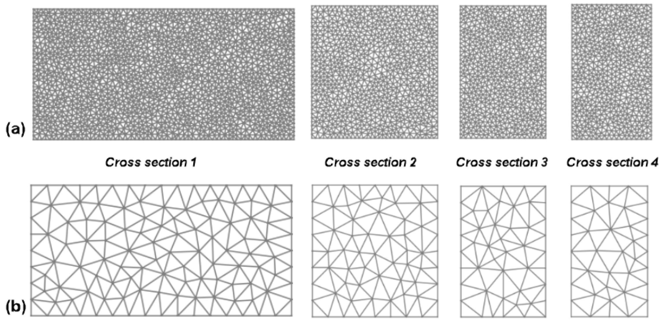
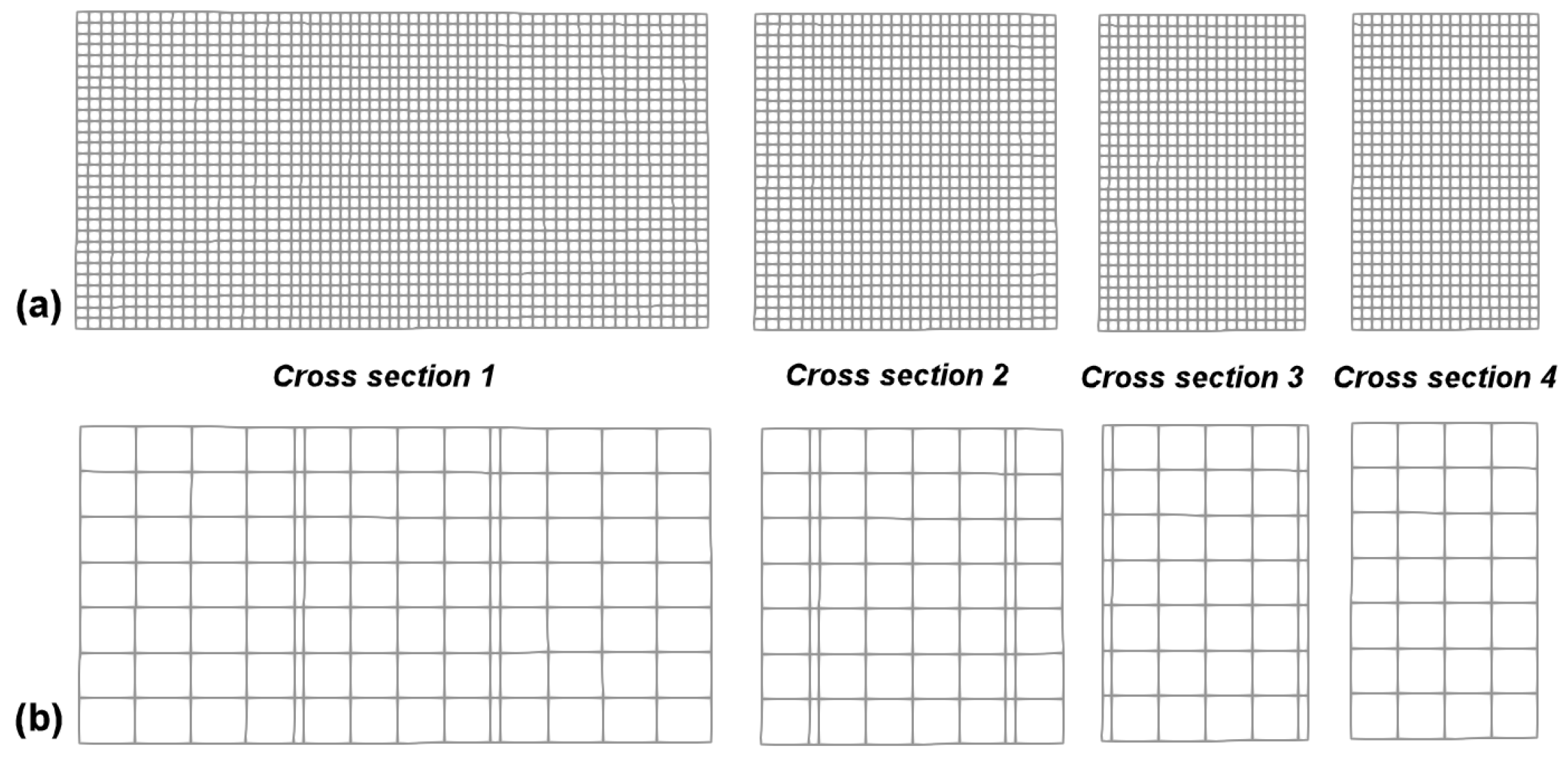
	Fine Meshes		Coarse Meshes
	Triangular	Quadrilateral	Triangular	Quadrilateral
Cross-section 1:	6717	6785	429	435
Cross-section 2:	3413	3481	245	255
Cross-section 3:	2563	2537	168	195
Cross-section 4:	2309	2301	141	135

shows the number of d.o.f. for each fine mesh (leftmost double column). As can be seen, 200 TE and 200 TM modes can be accurately computed with this high number of d.o.f. The reason for choosing 200 TE modes and 200 TM modes in each discontinuity is for mere comparison when using fewer number of modes computed with coarser meshes made up of triangular and quadrilateral elements. It is beyond the scope of this work to address well-known issues related to the MM convergence with respect to the number of modes. To that effect, it just suffices to know that 200 TE and 200 TM modes are well beyond the minimum number of modes required to reach convergence in this device. As a proof, Figure 9 shows the reflection coefficient magnitude (dB) achieved with MM for this number of modes computed with the aforementioned fine meshes. As expected, they are identical. Since all cross-sections of this structure are rectangular and thus have analytical solution for the modes, the analytical MM result for the same number of modes is also shown in Figure 9 for comparison purposes, corroborating that with the fine meshes and such number of modes the H-plane rectangular waveguide filter is correctly simulated and that the results are grid-independent.

Now, coarser meshes with a similar number of d.o.f. are considered for the cross-sections of this device. They are shown in the lower rows of Figure 7 (triangular) and Figure 8 (quadrilateral). Details on the number of d.o.f. for these coarse meshes (with elements of order 1) are also listed in Table 2 (rightmost double column). With these meshes, 60 TE and 60 TM modes are considered for the MM procedure in each discontinuity. This number is chosen so that the minimum number of d.o.f. in the smallest cross-sections (135 for quadrilateral elements and 141 for triangular elements) is well beyond the number of modes to be computed, ensuring that the eigenvalue/eigenvector matrix system in (4) converges properly. Figure 10 shows the MM results for these two sets of coarse meshes, together with the reference result obtained with any of the fine meshes (triangular or quadrilateral elements). It is shown how for fewer d.o.f., quadrilateral elements achieve results closer to the reference reflection coefficient magnitude (obtained with 200 TE and 200 TM modes accurately computed with any of the fine meshes). On the other hand, using triangular elements results in increased lobes in the simulated reflection coefficient magnitude of the passband region. This means that using a structured quadrilateral mesh for these simple rectangular cross-sections enhances the accuracy (in this case, for the first 60 TE and 60 TM modes), implying that fewer computational resources are required if quadrilateral elements are used. Indeed, for this example, reducing the number of elements from the fine to the coarse meshes and, correspondingly, the number of modes from 200 to 60 (both TE and TM) resulted in a $18\times –20\times$ speedup factor of the hybrid FEM-MM simulation independent of frequency (i.e., to obtain the elements of the normalized cross-product matrix (13)) for both type of elements (triangular and quadrilateral). However, in view of the results in Figure 10, only the use of quadrilateral elements retains a high degree of precision with respect to the reference return loss.

The second studied device is a bandpass filter composed of ridge waveguide cross-sections [35]. In this case, these cross-sections do not have analytical solutions for their modes, so the use of a numerical method to hybridize with MM is imperative. This filter is shown in Figure 11. The procedure applied here is the same one as explained for rectangular waveguide H-plane filter. First, the response for a very high d.o.f. density is obtained using fine meshes made of triangular and quadrilateral elements of order 1, shown respectively in Figure 12 and Figure 13 (upper rows). Details of the number of d.o.f. for each cross-section are shown in

Table 3. Number of d.o.f. for the meshes of each cross-section of the ridge waveguide filter depicted in Figure 12 and Figure 13.

	Fine Meshes		Coarse Meshes
	Triangular	Quadrilateral	Triangular	Quadrilateral
Cross-section 1:	5261	5693	446	389
Cross-section 2:	3317	3645	284	293

(leftmost double column). For the MM procedure, the number of modes for all the cross-sections is set to the same as the previous example, 200 TE and TM modes, for the sake of simplicity. These converged results, which are once again grid independent, are shown in Figure 14. As can be seen, there is virtually no difference between elements. The reflection coefficient computed with the hybrid MM-FEM procedure for these fine meshes becomes the reference for comparison with lower mesh densities and number of modes.

In Figure 15, the reflection coefficient magnitude obtained with 150 TE and 150 TM modes in the MM procedure for the coarse meshes shown in the lower rows of Figure 12 (triangular) and Figure 13 (quadrilateral) are compared against the previous fine-mesh baseline. The behaviour at the lower part of the passband is similar, but for the higher-frequency lobes the difference in response between triangular and quadrilateral elements becomes more pronounced, which implies that higher-order modes are being more accurately computed for quadrilateral elements. Details of the number of d.o.f. (elements of order 1, as well) for each cross-section in the coarse meshes are shown in Table 3 (rightmost double column). For this example, the speedup factor achieved with the reduction in the number of d.o.f. and modes is $13\times –14\times$ for both types of elements. However, as in the previous example, only the use of quadrilateral elements ensures achieving similar results to the converged fine-mesh response.

The presented examples show how it is, in general, more appropriate to use quadrilateral elements when dealing with Manhattan-type structures. This is because, given comparable d.o.f. counts and computational times, the use of quadrilateral elements yield more accurate results. It is safe to say that, in these cases, the quadrilateral cell type has an advantage over the triangular finite element, especially when doing fast or iterating simulations.

4. Conclusions

A comparison between the results of using quadrilateral and triangular cells for the analysis of waveguide devices made up of Manhattan-type cross-sections has been carried out from two different perspectives. In the first approach, three homogeneous waveguides are selected for the computation of their modal spectrum, with special focus on degenerate mode calculation and identification. All the computations in these analyses have been done trying to preserve the same number of d.o.f. (using Lagrange elements of order 2) both for triangular and quadrilateral meshes. Results show how the relative error for higher-order degenerate modes remains low (up to machine precision) only if using quadrilateral cells, which makes the identification of this degeneracy easier. In the second approach, the advantage of using quadrilateral cells is challenged by analyzing two waveguide bandpass filters with the use of a hybrid MM-FEM method. In this hybrid method, modes are computed with elements (either triangular or quadrilateral) of order 1. Firstly, fine meshes are used with both types of cells and a similar number of d.o.f. to compute a reference response, which is identical no matter which type of element (triangular or quadrilateral is used). Secondly, the response is obtained with the use of coarser meshes with a lower number of d.o.f. (which entails reducing the number of modes in the MM procedure). Results show how only the use of quadrilateral elements ensures achieving results comparable to the converged fine-mesh results.

Future work may include similar studies related to the accuracy of hexahedral vs. tetrahedral meshes both for the FEM solution of 3D electromagnetic eigenproblems (i.e., cavities mode spectrum) [6,7] and for other hybrid FEM approaches for the analysis of complex 3D waveguide structures, i.e., through hybrid FEM-MM [36] or hybrid FEM-beam propagation method [37].

References

- Reddy, J. An Introduction to the Finite Element Method; McGraw-Hill: New York, NY, USA, 2005. [Google Scholar]
- Zienkiewicz, O.C.; Taylor, R.L.; Zhu, J.Z. The Finite Element Method: Its Basis and Fundamentals, 6th ed.; Butterworth-Heinemann: Oxford, UK, 2005. [Google Scholar]
- Marin, M.; Hobiny, A.; Abbas, I. Finite Element Analysis of Nonlinear Bioheat Model in Skin Tissue Due to External Thermal Sources. Mathematics 2021, 9, 1459. [Google Scholar] [CrossRef]
- Nyka, K. Diagonalized Macromodels in Finite Element Method for Fast Electromagnetic Analysis of Waveguide Components. Electronics 2019, 8, 260. [Google Scholar] [CrossRef] [Green Version]
- Lobry, J. A FEM-Green Approach for Magnetic Field Problems with Open Boundaries. Mathematics 2021, 9, 1662. [Google Scholar] [CrossRef]
- Pelosi, G.; Coccioli, R.; Selleri, S. Quick Finite Elements for Electromagnetic Waves; Artech House: Norwood, MA, USA, 2009. [Google Scholar]
- Jin, J. The Finite Element Method in Electromagnetics; Wiley: Hoboken, NJ, USA, 2015. [Google Scholar]
- Uher, J.; Bornemann, J.; Rosenberg, U. Waveguide Components for Antenna Feed Systems: Theory and CAD; Artech House: Boston, FL, USA, 1993. [Google Scholar]
- Arndt, F. Efficient EM CAD and optimization by advanced hybrid methods: Science and product. In Proceedings of the 5th European Conference on Antennas and Propagation (EUCAP), Rome, Italy, 11–15 April 2011; pp. 2847–2851. [Google Scholar]
- Beyer, R.; Arndt, F. Efficient modal analysis of waveguide filters including the orthogonal mode coupling elements by an MM/FE method. IEEE Microw. Guid. Wave Lett. 1995, 5, 9–11. [Google Scholar] [CrossRef]
- Zapata, J.; García, J. Analysis of passive microwave structures by a combined finite element-generalized scattering matrix method. In Proceedings of the North American Radio Science Meeting, London, ON, Canada, 24–28 June 1991; p. 146. [Google Scholar]
- Zapata, J.; Garcia, J.; Valor, L.; Garai, J.M. Field-theory analysis of cross-iris coupling in circular waveguide resonators. Microw. Opt. Technol. Lett. 1993, 6, 905–907. [Google Scholar] [CrossRef]
- Montejo-Garai, J.; Valor, L.; Garcia, J.; Zapata, J. A full-wave analysis of tuning and coupling posts in dual-mode circular waveguide filters. Microw. Opt. Technol. Lett. 1994, 7, 505–507. [Google Scholar] [CrossRef]
- Córcoles, J.; Morán-López, A.; Ruiz-Cruz, J.A. Nested 2D finite-element function-spaces formulation for the mode-matching problem of arbitrary cross-section waveguide devices. Appl. Math. Model. 2018, 60, 286–299. [Google Scholar] [CrossRef]
- Collin, R.E. Foundations for Microwave Engineering, 2nd ed.; Wiley-IEEE Press: Hoboken, NJ, USA, 2001. [Google Scholar]
- Silvester, P. Finite element solution of homogeneous waveguide problems. Alta Freq. 1969, 38, 313–317. [Google Scholar]
- Silvester, P. A general high-order finite-element waveguide analysis program. IEEE Trans. Microw. Theory Tech. 1969, 21, 538–542. [Google Scholar] [CrossRef]
- Konrad, A. Vector Variational Formulation of Electromagnetic Fields in Anisotropic Media. IEEE Trans. Microw. Theory Tech. 1976, 24, 553–559. [Google Scholar] [CrossRef]
- Dillon, B.M.; Webb, J.P. A comparison of formulations for the vector finite element analysis of waveguides. IEEE Trans. Microw. Theory Tech. 1994, 42, 308–316. [Google Scholar] [CrossRef]
- Miniowitz, R.; Webb, J.P. Covariant-projection quadrilateral elements for the analysis of waveguides with sharp edges. IEEE Trans. Microw. Theory Tech. 1991, 39, 501–505. [Google Scholar] [CrossRef]
- Shivaram, K.T.; Harshitha, L.M.P.; Chethana, H.P.; Nidhi, K. Finite element mesh generation technique for numerical computation of cutoff wave numbers in rectangular and L-shaped waveguide. In Proceedings of the 3rd International Conference on Inventive Computation Technologies (ICICT), Coimbatore, India, 15–16 November 2018; pp. 704–706. [Google Scholar]
- Blanc-Castillo, F.; Salazar-Palma, M.; Garcia-Castillo, L.E. Linear and second order edge-Lagrange finite elements for efficient analysis of waveguide structures with curved contours. In Proceedings of the Microwave Conference 1995, 25th European, Bologna, Italy, 4 September 1995; Volume 1, pp. 444–448. [Google Scholar]
- Khodapanah, E. Efficient 2-D Finite-Element Solution of Vector Wave Equation in a class of Curved Polygons. IEEE Trans. Antennas Propag. 2016, 64, 3687–3691. [Google Scholar] [CrossRef]
- Garcia-Contreras, G.; Córcoles, J.; Ruiz-Cruz, J.A. Degeneracy-Discriminating Modal FEM Computation in Higher Order Rotationally Symmetric Waveguides. IEEE Trans. Antennas Propag. 2021, 69, 8003–8008. [Google Scholar] [CrossRef]
- Lee, J.-F. Finite element analysis of lossy dielectric waveguides. IEEE Trans. Microw. Theory Tech. 1994, 42, 1025–1031. [Google Scholar] [CrossRef]
- Polstyanko, S.; Lee, J.-F. H1(curl) tangential vector finite element method for modeling anisotropic optical fibers. J. Light. Technol. 1995, 13, 2290–2295. [Google Scholar] [CrossRef]
- Lee, J.-S.; Shin, S.-Y. On the validity of the effective-index method for rectangular dielectric waveguides. J. Light. Technol. 1993, 11, 1320–1324. [Google Scholar] [CrossRef]
- Kim, C.M.; Jung, B.G.; Lee, C.W. Analysis of dielectric rectangular waveguide by the modified effective index method. Electron. Lett. 1986, 22, 296. [Google Scholar] [CrossRef]
- Adriano, R.; Facco, W.G.; Silva, E.J. A Modified Plane Wave Enrichment to Solve 2-D Electromagnetic Problems Using the Generalized Finite-Element Method. IEEE Trans. Magn. 2015, 51, 1–4. [Google Scholar] [CrossRef]
- Strouboulis, T.; Babuška, I.; Hidajat, R. The generalized finite element method for Helmholtz equation: Theory, computation, and open problems Computer Methods. Appl. Mech. Eng. 2006, 195, 4711–4731. [Google Scholar] [CrossRef]
- Logg, A.; Mardal, K.A.; Wells, G. Automated Solution of Differential Equations by the Finite Element Method; Springer: Berlin/Heidelberg, Germany, 2012. [Google Scholar]
- Wexler, A. Solution of waveguide discontinuities by modal analysis. IEEE Trans. Microw. Theory Tech. 1967, 15, 508–517. [Google Scholar] [CrossRef]
- Guglielmi, M.; Sorrentino, R.; Conciauro, G. Advanced Modal Analysis: Cad Techniques for Waveguide Components and Filter; John Wiley & Sons, Inc.: Hoboken, NJ, USA, 1999; Volume 127, p. 128. [Google Scholar]
- Ruiz-Cruz, J.A.; Montejo-Garai, J.R.; Rebollar, J.M. Computer aided design of waveguide devices by mode-matching methods. In Passive Microwave Components and Antennas; Zhurbenko, V., Ed.; InTech: London, UK, 2010; pp. 117–140. [Google Scholar]
- Ruiz-Cruz, J.A.; Zhang, Y.; Zaki, K.A.; Piloto, A.J.; Tallo, J. Ultra-Wideband LTCC Ridge Waveguide Filters. IEEE Microw. Wirel. Components Lett. 2007, 17, 115–117. [Google Scholar] [CrossRef]
- Rubio, J.; Arroyo, J.; Zapata, J. SFELP-an efficient methodology for microwave circuit analysis. IEEE Trans. Microw. Theory Tech. 2001, 49, 509–516. [Google Scholar] [CrossRef]
- Tsuji, Y.; Koshiba, M.; Shiraishi, T. Finite element beam propagation method for three-dimensional optical waveguide structures. J. Light. Technol. 1997, 15, 1728–1734. [Google Scholar] [CrossRef]