Distributed Fusion Estimation in Network Systems Subject to Random Delays and Deception Attacks

Abstract

This paper focuses on the distributed fusion estimation problem in which a signal transmitted over wireless sensor networks is subject to deception attacks and random delays. We assume that each sensor can suffer attacks that may corrupt and/or modify the output measurements. In addition, communication failures between sensors and their local processors can delay the receipt of processed measurements. The randomness of attacks and transmission delays is modelled by different Bernoulli random variables with known probabilities of success. According to these characteristics of the sensor networks and assuming that the measurement noises are cross-correlated at the same time step between sensors and are also correlated with the signal at the same and subsequent time steps, we derive a fusion estimation algorithm, including prediction and filtering, using the distributed fusion method. First, for each sensor, the local least-squares linear prediction and filtering algorithm are derived, using a covariance-based approach. Then, the distributed fusion predictor and the corresponding filter are obtained as the matrix-weighted linear combination of corresponding local estimators, checking that the mean squared error is minimised. A simulation example is then given to illustrate the effectiveness of the proposed algorithms.

1. Introduction

Wireless sensor networks (WSNs) are a growing focus of research, with applications in a wide variety of fields including industrial processes, signal processing, communications and navigation systems. In general, each WSN is composed of a large number of sensors that can be interconnected by wireless channels and also linked to the processing centre. While they are widely used, the structure of WSNs makes them vulnerable to external attacks and/or unreliability in data transmission. In this context, a topic that has attracted considerable attention is that of signal fusion estimation. This problem can be addressed by centralised or distributed fusion methods. Both are commonly used to tackle the question of fusion estimation; however, the distributed method is usually more suitable, since the structure of the sensors means that less online communication is required, because each local estimator is obtained using only its corresponding local data, and therefore manufacturing costs are reduced. Consequently, this method usually has stronger fault tolerance and lower calculation burdens than the centralised approach. Accordingly, the distributed fusion estimation problem has been of particular interest to researchers, and a large number of distributed fusion estimation algorithms have been developed, using different techniques, in the context of WSNs (see [1,2,3,4,5,6,7] and references therein).

As commented above, the characteristics of WSNs make them vulnerable to external attacks and hence less reliable. In general, three kinds of attack have been considered (classified according to the attack mechanisms and mathematical models involved): Denial-of-service (DoS) attacks, replay attacks and deception attacks. A DoS attack deteriorates system performance by temporarily or indefinitely interrupting the service, preventing information from reaching the destination. In a replay attack, the information is intercepted, captured and forwarded elsewhere, thus altering the system’s behaviour. Deception attacks tamper with the original signal measures by accessing the sensors and introducing false information. A problem of significant interest in WSNs subject to cyber-attacks is that of the distributed fusion estimation of the signal. This problem can be addressed in various ways, depending on the type of attack considered. Chen et al. [8] designed a distributed resilient filter for power systems exposed to DoS attacks and gain perturbations. Similarly, the distributed robust fusion estimation problem for systems under DoS attacks and uncertain covariances was studied by [9]. For replay attacks, [10] designed a recursive distributed Kalman fusion estimator focused on the linear minimum variance, for bandwidth-constrained cyber-physical systems. Finally, deception attacks are generally considered the most dangerous and complex types of aggression; for this reason, the scientific community is highly active in researching estimation problems for WSNs subject to this kind of attack. For instance, [11] developed a novel filter for a class of discrete time-delayed stochastic systems subject to the effects of both uniform quantisation and deception attacks. In this field, too, [12] considered a class of time-varying systems subject to multiplicative noises and deception attacks, with unknown but bounded disturbances, and designed an appropriate variance-constrained distributed filter. [13] derived a distributed $H_{\infty }$-consensus filter for a class of discrete time-varying systems subject to both multiplicative noises and deception attacks. In a related approach, assuming clustering sensor networks subject to random deception attacks, [14] considered distributed fusion filtering and fixed-point smoothing problems.

Another significant problem in WSNs is the limitation of network communication bandwidth, which can produce network congestion and hence delay reception of the measures at the processing centre, thus impairing the performance of the estimator. Accordingly, new algorithms must be developed to take these effects into account in distributed fusion estimation. In studies of one-step random delays modelled by Bernoulli random variables, various types of distributed fusion estimation algorithms have been proposed, assuming either that these variables are independent (see for example, [15,16,17,18]) or that they are correlated at consecutive sampling times [19,20]. In addition, various distributed fusion estimation algorithms describing random delays by Markov chains have been derived (see, for example, [21,22,23]).

Many early studies of the estimation problem in multi-sensor systems assumed that the system noises were white and uncorrelated. However, in practice, this assumption is not always realistic; for example, when all sensors observe a common target within a noisy environment, there may be cross-correlations between the different sensor noises. Cross-correlation between process and measurement noises can also arise, for example, when in a target tracking system both noises are dependent of the state of the system. In this respect, Li et al. [24] showed that if a discrete-time linear system is obtained from the discretisation of a continuous-time system, then the measurement noise is correlated with the system noise of the previous time step. These common situations in multi-sensor systems have led researchers to address the fusion estimation problem under the assumption of correlated noises. Thus, assuming that the measurement noises from different sensors are both cross-correlated and correlated with the system noise at the previous time step, Yan et al. [25] derived the optimal state estimator, in a sequential form and by means of distributed fusion. Similarly, ref. [26] developed globally optimal sequential and distributed fusion estimation algorithms assuming linear minimum variance. The distributed estimation problem has also been addressed when the noises between sensors are not correlated at the same instant, but the process and measurement noises are two-step cross-correlated; under this assumption, distributed filtering algorithms have been obtained assuming that the system is subject to stochastic uncertainties or multiplicative noises [27] and in systems with random matrices over a sensor network with a given topology [28].

Motivated by the above analysis, our aim in this paper is to address the distributed fusion estimation problem in WSNs subjected to the three situations described above, as often encountered in real life: Deception attacks, one-step random transmission delays and measurement noises cross-correlated between sensors and correlated with the signal. To the best of our knowledge, this problem has not been considered previously, although some papers have discussed deception attacks and delays or correlated noises. Specifically, for a single sensor, the estimation problem is studied assuming deception attacks and random communication delays in [29,30], and in a multi-sensor environment, ref. [31] investigated the distributed filtering problem in WSNs receiving deception attacks and when sensor additive noises are both cross-correlated and correlated with the process noise.

In this paper, we assume that each sensor of the WSN can suffer random attacks that modify the output measurements. The randomness of these attacks is modelled by independent random Bernoulli variables reflecting whether or not the attack succeeded in modifying the measure. Furthermore, the measurement noises from different sensors are cross-correlated at the same time step and are also correlated with the signal process at the same and subsequent time steps. Due to possible imperfections in communication channels, the processed measurements can be one-step delayed with different delay rates. Transmission delays, which occur randomly, are described by different random Bernoulli variables describing whether the processed measurements arrive on time, or are delayed by one sampling time. In this context, assuming that no signal evolution equation is available, a distributed fusion prediction and filtering algorithm is derived using the first and second-order moments of the signal and the processes involved in the observations. The design of the proposed distributed prediction and filtering estimators is structured in two stages. In the first, an innovation approach is used to obtain the local least-squares (LS) linear prediction and the filtering estimators. In the second stage, the information provided by the local estimators is combined to derive the fusion estimators; specifically, the distributed fusion predictor and filter are obtained as a matrix-weighted linear combination of the local LS linear estimators, using the mean squared error as the optimality criterion.

The rest of this paper is organised as follows. In the next section, we describe the model proposed and specify the assumptions under which the distributed fusion estimation problem is addressed. The distributed fusion prediction and filtering algorithm and the associated error covariance matrices, which provide a measure of the estimator performance, are then derived in Section 3. In order to illustrate the feasibility of the proposed distributed fusion estimators, a simulation example is given in Section 4. Finally, the main conclusions drawn are summarised in Section 5.

Notation. 

The notations used in this paper are standard. ${\mathbb{R}}^n$ and ${\mathbb{R}}^{n\times m}$ denote the n-dimensional Euclidean space and the set of all $n\times m$ matrices, respectively. If the dimensions of vectors or matrices are not explicitly stated, they are assumed to be compatible with algebraic operations. The shorthand $\left(A_1\right|\cdots \left|A_m\right)$ stands for a matrix partitioned into submatrices $A_i,i=1,\cdots ,m$. The Kronecker delta function is denoted as ${\delta }_{k,s}$. Finally, $L^{\left(i\right)}=L^{\left(ii\right)}$ is written for any function $L^{\left(ij\right)}$ depending on sensors i and j; similarly, for any function $G_{k,s},$ depending on the time instants k and s, we simply write $G_k$ when $k=s$.

2. Problem Formulation

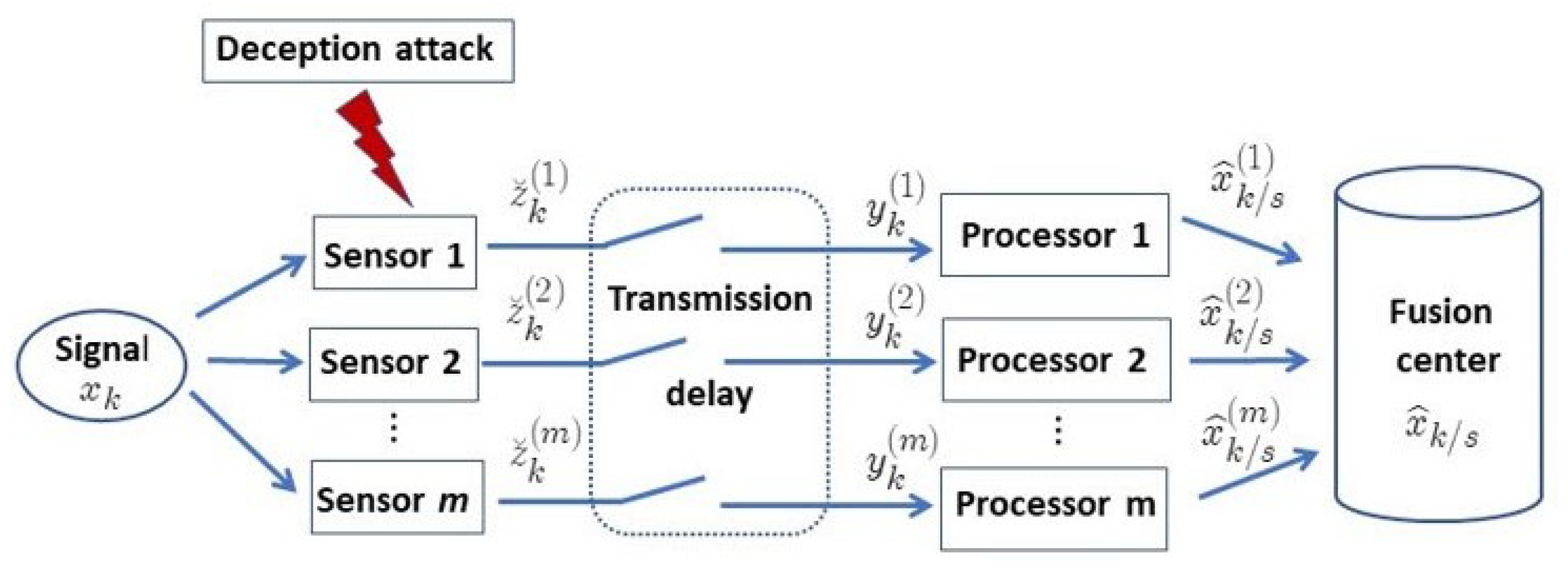
This paper considers the linear estimation problem of a discrete-time signal over WSNs subject to deception attacks, random delays and correlated noises. More specifically, the problem is to estimate a signal from the sensor measurements $z_k^{\left(i\right)},i=1,\dots ,m$, which are described by Equation (1). We assume that deception attacks are launched by potential adversaries, inserting false information that may perturb the real measurements. Assuming that the attacks may randomly succeed or not, the sensor-measured outputs subject to these attacks, ${\breve{z}}_k^{\left(i\right)}$, are modeled by (2). It is also assumed that each sensor transmits its outputs to a local processor over a packet-erasure channel, where one-step random delays can occur during transmission; the measures received by the local processors, $y_k^{\left(i\right)}$, are given by (5). The linear estimation problem is addressed using the distributed fusion method, by which each local processor produces LS linear predictors and filters, ${\widehat{x}}_{k/s}^{\left(i\right)},s=k-1,k,$ of the signal, $x_k$, based on the measures received from the corresponding sensor, $y_1^{\left(i\right)},\dots ,y_s^{\left(i\right)}$; afterwards, these estimators are transmitted, over perfect connections, to the fusion center, where new prediction and filtering estimators, ${\widehat{x}}_{k/s},s=k-1,k,$ are obtained as matrix-weighted linear combination of the local estimators using the mean squared error as the optimality criterion (see Figure 1).

2.1. Multisensor Measurement

Consider a networked system consisting of m sensors which measure a $n_x$-dimensional discrete-time signal $x_k$ according the following model:

$$z_k^{\left(i\right)}=H_k^{\left(i\right)}{x}_k+v_k^{\left(i\right)},k\ge 1,i=1,\cdots m,$$

(1)

where $z_k^{\left(i\right)}\in {\mathbb{R}}^{n_z},H_k^{\left(i\right)}\in {\mathbb{R}}^{n_z\times n_x}$ are known matrices and $v_k^{\left(i\right)}$ are the measurement noises.

The following assumptions on the measurement model (1) are required:

Assumption 1.

The $n_x$-dimensional signal $\left\{x_k,k\ge 1\right\}$ is a second-order process with zero mean and autocovariance function expressed in a separable form as follows:

$$E\left[x_k{x}_h^T\right]=A_k{B}_h^T,h\le k,$$

where $A_k,B_h\in {\mathbb{R}}^{n_x\times M}$ are known matrices.

Assumption 2.

The measurement noises $\left\{v_k^{\left(i\right)},k\ge 1\right\},i=1,\cdots ,m$, are white second-order processes with the following statistical properties:

$\left(i\right)$

$E\left[v_k^{\left(i\right)}\right]=0$ and their correlation functions are known and given by

$$E\left[v_k^{\left(i\right)}{v}_h^{\left(j\right)T}\right]=R_k^{\left(ij\right)}{\delta }_{k,h},i,j=1,\cdots ,m.$$

$\left(ii\right)$

For $i=1,\cdots ,m,\left\{v_k^{\left(i\right)},k\ge 1\right\},$ is correlated with the signal process $\left\{x_k,k\ge 1\right\}$ and its correlation function is expressed in separable form as

$$E\left[x_k{v}_h^{\left(i\right)T}\right]=\left\{\begin{array}{cc}{C}_k{D}_h^{\left(i\right)T},\hfill & h\le k,\hfill \\ 0,\hfill & h>k,\hfill \end{array}\right.$$

where $C_k\in {\mathbb{R}}^{n_x\times M^{\prime }}$ and $D_h^{\left(i\right)}\in {\mathbb{R}}^{n_z\times M^{\prime }}$ are known matrices.

Remark 1.

The general assumption of uncorrelation for the system noises is not always true and it can be restrictive in many real-world problems, where both correlation and cross-correlation of the noises may be present. Assumption 2 weakens this condition of uncorrelated noises. Concretely:

• The sensor noise cross-correlation specified in $\left(i\right)$ can be found, for example, when the signal process is observed by sensors that operate in a common noisy environment, or when the noises are state dependent; in this case, the cross-correlation between the process noise and the sensor noises leads to correlation between the different sensor noises. Moreover, after augmenting a system subject to uncertainties such as random delays or packet-dropouts, the transformed system presents correlated noises.
• Condition $\left(ii\right)$ allows us to consider models in which the sensor noises are correlated with the process noise at the previous time (see Section 4). One of the most common situations in which this type of correlation occurs is in the discretisation of continuous-time systems; actually, if a discrete-time linear system is obtained from the discretisation of a continuous-time system, then the measurement noise is correlated with the process noise at the previous time.

2.2. Deception Attack Model

As discussed above, the measurement process can be subject to attacks launched by malicious attackers. Specifically, at each sensor, attackers could inject false information that would degrade or deteriorate the real measurement. If deception attacks are launched randomly, the output measure may or may not be modified; therefore, the mathematical model for current output after a randomly occurring deception attack is modelled as:

$${\breve{z}}_k^{\left(i\right)}=z_k^{\left(i\right)}+{\beta }_k^{\left(i\right)}{\xi }_k^{\left(i\right)},k\ge 1,i=1,\cdots ,m,$$

(2)

where $\left\{{\beta }_k^{\left(i\right)},k\ge 1\right\},i=1,\cdots ,m,$ are sequences of Bernoulli random variables, which model the success, ${\beta }_k^{\left(i\right)}=1$, or failure, ${\beta }_k^{\left(i\right)}=0$, of the attack on the $ith$-sensor and ${\xi }_k^{\left(i\right)}$ denotes the deception attack signal sent by adversaries to the $ith$-sensor, which can be described as follows:

$${\xi }_k^{\left(i\right)}=-z_k^{\left(i\right)}+{\epsilon }_k^{\left(i\right)},k\ge 1,i=1,\cdots ,m,$$

(3)

where ${\epsilon }_k^{\left(i\right)}$ represents a random deception signal, which is inaccessible to the defenders.

According to the deception attacks (3), the attacked measurement outputs (2) can be rewritten as:

$${\breve{z}}_k^{\left(i\right)}=(1-{\beta }_k^{\left(i\right)})z_k^{\left(i\right)}+{\beta }_k^{\left(i\right)}{\epsilon }_k^{\left(i\right)},k\ge 1,i=1,\cdots ,m.$$

(4)

The following assumptions are set on the sequences of random variables that model the occurrence or otherwise of the attack and the deception signal:

Assumption 3.

$\left\{{\beta }_k^{\left(i\right)},k\ge 1\right\},i=1,\cdots ,m$, are independent sequences of independent Bernoulli random variables with known success probabilities $P({\beta }_k^{\left(i\right)}=1)={\overline{\beta }}_k^{\left(i\right)},k\ge 1.$

Assumption 4.

$\left\{{\epsilon }_k^{\left(i\right)},k\ge 1\right\},i=1,\cdots ,m,$ are independent white second-order processes with zero-mean and known covariance matrices $E\left[{\epsilon }_k^{\left(i\right)}{\epsilon }_h^{\left(j\right)T}\right]=T_k^{\left(ij\right)}{\delta }_{k,h}.$

Remark 2.

For various reasons, such as the possible presence of safety protection devices, the attacks launched by adversaries are not always successful. From the defender’s perspective, the uncertainty about the success or failure of a deception attack should be considered random and included in the model with the certain-success rates, different for every sensor and every time instant. The nature of the uncertainty (successful or failed attacks) suggests that the randomness should be modelled using different sequences of random binary variables,$\left\{{\beta }_k^{\left(i\right)},k\ge 1\right\}$, each taking the value 0 (${\beta }_k^{\left(i\right)}=0$, meaning that the attack against the $ith$-sensor at time k has failed) or the value 1 (${\beta }_k^{\left(i\right)}=1$ representing the success of the $ith$-sensor attack at time k). Clearly, therefore, the measurement output of the $ith$-sensor at time k, ${\breve{z}}_k^{\left(i\right)}$, is modelled by (3); that is, it is only noise, ${\breve{z}}_k^{\left(i\right)}={\epsilon }_k^{\left(i\right)}$, if ${\beta }_k^{\left(i\right)}=1$ (successful attack) or, alternatively, it is the real measure, ${\breve{z}}_k^{\left(i\right)}=z_k^{\left(i\right)}$, if ${\beta }_k^{\left(i\right)}=0$ (failed attack). Assumption 3 on $\left\{{\beta }_k^{\left(i\right)},k\ge 1\right\}$ specifies the independence of the success or failure of attacks against different sensors or at different times. Consequently, under this assumption, each measurement output is either the real measure or consists only of noise, regardless of the other.

2.3. Randomly Delayed Observations

It is assumed that the measures arriving from each sensor to its processing centre may have suffered delays during the transmission process, due to possible imperfections in the communication channels. For each sensor, the absence or presence of delays in the transmission is modelled by different sequences of Bernoulli variables describing whether the measures arrive on time or are delayed by one sampling time; thus, the measure to be processed at time k is ${\breve{z}}_k^{\left(i\right)}$ or ${\breve{z}}_{k-1}^{\left(i\right)}$. In addition, it is assumed that at the initial instant the actual outputs are always available. Therefore, our mathematical model of randomly one-step delayed received measures is described by

$$\begin{array}{c}{y}_k^{\left(i\right)}=(1-{\gamma }_k^{\left(i\right)}){\breve{z}}_k^{\left(i\right)}+{\gamma }_k^{\left(i\right)}{\breve{z}}_{k-1}^{\left(i\right)},k\ge 2;y_1^{\left(i\right)}={\breve{z}}_1^{\left(i\right)},i=1,\cdots ,m,\hfill \end{array}$$

(5)

and the following assumption is made for the random variables ${\gamma }_k^{\left(i\right)}$ modelling the delays:

Assumption 5.

$\left\{{\gamma }_k^{\left(i\right)},k\ge 2\right\},i=1,\cdots ,m$, are independent sequences of independent Bernoulli random variables with known success probabilities $P({\gamma }_k^{\left(i\right)}=1)={\overline{\gamma }}_k^{\left(i\right)},k\ge 2.$

Finally, the following assumption is made about the signal and processes involved in the measurement model used to derive the LS linear estimators.

Assumption 6.

For $i=1,\cdots ,m,$ the processes $\left(\left\{x_k,k\ge 1\right\},\left\{v_k^{\left(i\right)},k\ge 1\right\}\right),\left\{{\epsilon }_k^{\left(i\right)},k\ge 1\right\},$$\left\{{\beta }_k^{\left(i\right)},k\ge 1\right\}$ and $\left\{{\gamma }_k^{\left(i\right)},k\ge 2\right\}$ are mutually independent.

From the previous assumptions about the measurement, attacked measurement and observation processes, the expressions of their second order moments are deduced in the following lemma.

Lemma 1.

Under the model assumptions, the following statistical properties are satisfied:

$\left(i\right)$

The measurement processes $\left\{z_k^{\left(i\right)},k\ge 1\right\},i=1,\cdots ,m$, have zero-mean and their covariance functions, ${\Sigma }_{k,h}^{z^{\left(ij\right)}}\equiv E\left[z_k^{\left(i\right)}{z}_h^{\left(j\right)T}\right]$, are given by

$${\Sigma }_{k,h}^{z^{\left(ij\right)}}=H_k^{\left(i\right)}{A}_k{B}_h^T{H}_h^{\left(j\right)T}+R_k^{\left(ij\right)}{\delta }_{k,h}+H_k^{\left(i\right)}{C}_k{D}_h^{\left(j\right)T}+D_k^{\left(i\right)}{C}_k^T{H}_h^{\left(j\right)T}{\delta }_{k,h},1\le h\le k.$$

$\left(ii\right)$

The measurements $\left\{{\breve{z}}_k^{\left(i\right)},k\ge 1\right\},i=1,\cdots ,m,$ are zero-mean processes with

$$\begin{array}{c}{\Sigma }_k^{{\breve{z}}^{\left(i\right)}}\equiv E\left[{\breve{z}}_k^{\left(i\right)}{\breve{z}}_k^{\left(i\right)T}\right]=(1-{\overline{\beta }}_k^{\left(i\right)}){\Sigma }_k^{z^{\left(i\right)}}+{\overline{\beta }}_k^{\left(i\right)}{T}_k^{\left(i\right)},k\ge 1.\hfill \\ {\Sigma }_{k,h}^{{\breve{z}}^{\left(i\right)}}\equiv E\left[{\breve{z}}_k^{\left(i\right)}{\breve{z}}_h^{\left(i\right)T}\right]=(1-{\overline{\beta }}_k^{\left(i\right)})(1-{\overline{\beta }}_h^{\left(i\right)}){\Sigma }_{k,h}^{z^{\left(i\right)}},k,h\ge 1;h\ne k.\hfill \\ {\Sigma }_{k,h}^{{\breve{z}}^{\left(ij\right)}}\equiv E\left[{\breve{z}}_k^{\left(i\right)}{\breve{z}}_h^{\left(j\right)T}\right]=(1-{\overline{\beta }}_k^{\left(i\right)})(1-{\overline{\beta }}_h^{\left(j\right)}){\Sigma }_{k,h}^{z^{\left(ij\right)}}+{\overline{\beta }}_k^{\left(i\right)}{\overline{\beta }}_h^{\left(j\right)}{T}_k^{\left(ij\right)}{\delta }_{k,h},k,h\ge 1;j\ne i.\hfill \end{array}$$

$\left(iii\right)$

The observation processes $\left\{y_k^{\left(i\right)},k\ge 1\right\},i=1,\cdots ,m,$ have zero-mean and their covariance functions, ${\Sigma }_{k,h}^{y^{\left(ij\right)}}\equiv E\left[y_k^{\left(i\right)}{y}_h^{\left(j\right)T}\right]$, satisfy:

•

For $i=j$

$$\begin{gathered} \begin{array}{c}{\Sigma }_k^{y^{\left(i\right)}}=(1-{\overline{\gamma }}_k^{\left(i\right)}){\Sigma }_k^{{\breve{z}}^{\left(i\right)}}+{\overline{\gamma }}_k^{\left(i\right)}{\Sigma }_{k-1}^{{\breve{z}}^{\left(i\right)}},k\ge 2;{\Sigma }_1^{y^{\left(i\right)}}={\Sigma }_1^{{\breve{z}}^{\left(i\right)}}.\hfill \end{array} \\ {\Sigma }_{k,h}^{y^{\left(i\right)}}=(1-{\overline{\gamma }}_k^{\left(i\right)})(1-{\overline{\gamma }}_h^{\left(i\right)}){\Sigma }_{k,h}^{{\breve{z}}^{\left(i\right)}}+(1-{\overline{\gamma }}_k^{\left(i\right)}){\overline{\gamma }}_h^{\left(i\right)}{\Sigma }_{k,h-1}^{{\breve{z}}^{\left(i\right)}}+{\overline{\gamma }}_k^{\left(i\right)}(1-{\overline{\gamma }}_h^{\left(i\right)}){\Sigma }_{k-1,h}^{{\breve{z}}^{\left(i\right)}} \\ +{\overline{\gamma }}_k^{\left(i\right)}{\overline{\gamma }}_h^{\left(i\right)}{\Sigma }_{k-1,h-1}^{{\breve{z}}^{\left(i\right)}},1<h<k;{\Sigma }_{k,1}^{y^{\left(i\right)}}=(1-{\overline{\gamma }}_k^{\left(i\right)}){\Sigma }_{k,1}^{{\breve{z}}^{\left(i\right)}}+{\overline{\gamma }}_k^{\left(i\right)}{\Sigma }_{k-1,1}^{{\breve{z}}^{\left(i\right)}}k\ge 2. \end{gathered}$$

•

For $i\ne j$

$\begin{array}{c}{\Sigma }_{k,h}^{y^{\left(ij\right)}}=(1-{\overline{\gamma }}_k^{\left(i\right)})(1-{\overline{\gamma }}_h^{\left(j\right)}){\Sigma }_{k,h}^{{\breve{z}}^{\left(ij\right)}}+(1-{\overline{\gamma }}_k^{\left(i\right)}){\overline{\gamma }}_h^{\left(j\right)}{\Sigma }_{k,h-1}^{{\breve{z}}^{\left(ij\right)}}+{\overline{\gamma }}_k^{\left(i\right)}(1-{\overline{\gamma }}_h^{\left(j\right)}){\Sigma }_{k-1,h}^{{\breve{z}}^{\left(ij\right)}}\hfill \\ +{\overline{\gamma }}_k^{\left(i\right)}{\overline{\gamma }}_h^{\left(j\right)}{\Sigma }_{k-1,h-1}^{{\breve{z}}^{\left(ij\right)}},1<h\le k;\hfill \\ {\Sigma }_{k,1}^{y^{\left(ij\right)}}=(1-{\overline{\gamma }}_k^{\left(i\right)}){\Sigma }_{k,1}^{{\breve{z}}^{\left(ij\right)}}+{\overline{\gamma }}_k^{\left(i\right)}{\Sigma }_{k-1,1}^{{\breve{z}}^{\left(ij\right)}},k\ge 2;{\Sigma }_1^{y^{\left(ij\right)}}={\Sigma }_1^{{\breve{z}}^{\left(ij\right)}}.\hfill \end{array}$

Proof. 

These statistical properties are easily obtained taking into account Equations (1), (4) and (5), and model Assumptions (1)–(6). □

3. Least-Squares Linear Distributed Fusion Estimation Problem

The LS linear estimation problem of the signal from the observations coming from the m sensors is addressed by the distributed fusion method. This method is structured in two stages: The first consists of obtaining, for each sensor, LS linear estimators; in the second one, the distributed fusion estimators are calculated as matrix-weight linear combination of the local ones, using the LS optimisation criterion. Following this methodology, algorithms for the prediction and filtering problems are developed below.

3.1. Stage One: LS Local Prediction and Filtering Algorithm

In this stage, our aim is to obtain a recursive algorithm for the local estimators of the signal $x_k$ based on the observations $\left\{y_1^{\left(i\right)},\cdots ,y_s^{\left(i\right)}\right\}$, for $s\le k,$ applying an innovation approach. Under this approach, the observation process is transformed, by an orthogonalisation procedure, into an equivalent one that provides the same information; this is termed the innovation process. The innovation at time k is defined as ${\mu }_k^{\left(i\right)}=y_k^{\left(i\right)}-{\widehat{y}}_{k/k-1}^{\left(i\right)},$ where ${\widehat{y}}_{k/k-1}^{\left(i\right)}$ is the one-stage observation predictor. Due to this equivalence, the local estimator of a vector $u_k$ based on the observations $\left\{y_1^{\left(i\right)},\cdots ,y_s^{\left(i\right)}\right\}$ can be expressed as a linear combination of the innovations $\left\{{\mu }_1^{\left(i\right)},\cdots ,{\mu }_s^{\left(i\right)}\right\},$ as follows:

$${\displaystyle {\widehat{u}}_{k/s}^{\left(i\right)}=\sum _{h=1}^{s}E\left[u_k{\mu }_h^{\left(i\right)T}\right]{\Pi }_h^{\left(i\right)-1}{\mu }_h^{\left(i\right)},}$$

(6)

where ${\Pi }_h^{\left(i\right)}\equiv E\left[{\mu }_h^{\left(i\right)}{\mu }_h^{\left(i\right)T}\right]$ denotes the innovation covariance matrix.

Then, our first objective is to find an adequate expression for the innovations ${\mu }_h^{\left(i\right)}=y_h^{\left(i\right)}-{\widehat{y}}_{h/h-1}^{\left(i\right)},h\le s$, or, equivalently, for the one-stage observation predictors ${\widehat{y}}_{h/h-1}^{\left(i\right)}$, which simplifies the general expression of the local estimators of the signal, ${\displaystyle {\widehat{x}}_{k/s}^{\left(i\right)}=\sum _{h=1}^{s}E\left[x_k{\mu }_h^{\left(i\right)T}\right]{\Pi }_h^{\left(i\right)-1}{\mu }_h^{\left(i\right)},s\le k}$. This expression of the innovations will enable us to obtain the coefficients $E\left[x_k{\mu }_h^{\left(i\right)T}\right]$ and the innovation covariance matrices ${\Pi }_h^{\left(i\right)}$ that appear in the above expression of ${\widehat{x}}_{k/s}^{\left(i\right)}$.

One-stage observation predictor.

To facilitate the derivation of the one-stage observation predictor, we rewrite the observation expression (5) as

$$\begin{array}{c}{y}_k^{\left(i\right)}=(1-{\gamma }_k^{\left(i\right)})(1-{\beta }_k^{\left(i\right)})(H_k^{\left(i\right)}{x}_k+v_k^{\left(i\right)})+(1-{\gamma }_k^{\left(i\right)}){\beta }_k^{\left(i\right)}{\epsilon }_k^{\left(i\right)}+{\gamma }_k^{\left(i\right)}(1-{\overline{\beta }}_{k-1}^{\left(i\right)})H_{k-1}^{\left(i\right)}{x}_{k-1}+w_{k-1}^{\left(i\right)},k\ge 2;\hfill \\ y_1^{\left(i\right)}={\breve{z}}_1^{\left(i\right)},\hfill \end{array}$$

(7)

where

$$w_{k-1}^{\left(i\right)}={\gamma }_k^{\left(i\right)}({\overline{\beta }}_{k-1}^{\left(i\right)}-{\beta }_{k-1}^{\left(i\right)})H_{k-1}^{\left(i\right)}{x}_{k-1}+{\gamma }_k^{\left(i\right)}(1-{\beta }_{k-1}^{\left(i\right)})v_{k-1}^{\left(i\right)}+{\gamma }_k^{\left(i\right)}{\beta }_{k-1}^{\left(i\right)}{\epsilon }_{k-1}^{\left(i\right)},k\ge 2.$$

Then, taking into account the independence assumption and the Orthogonal Projection Lemma (OPL), it is clear that the one-stage observation predictor is given by

$$\begin{array}{c}{\widehat{y}}_{k/k-1}^{\left(i\right)}=(1-{\overline{\gamma }}_k^{\left(i\right)})(1-{\overline{\beta }}_k^{\left(i\right)})H_k^{\left(i\right)}{\widehat{x}}_{k/k-1}^{\left(i\right)}+{\overline{\gamma }}_k^{\left(i\right)}(1-{\overline{\beta }}_{k-1}^{\left(i\right)})H_{k-1}^{\left(i\right)}{\widehat{x}}_{k-1/k-1}^{\left(i\right)}+{\widehat{w}}_{k-1/k-1}^{\left(i\right)},k\ge 2,\hfill \end{array}$$

where ${\widehat{x}}_{k/k-1}^{\left(i\right)}$ and ${\widehat{x}}_{k-1/k-1}^{\left(i\right)}$ are the predictor and filter of the signal, respectively, and ${\widehat{w}}_{k-1/k-1}^{\left(i\right)}$ is the filter of $w_{k-1}^{\left(i\right)}$.

From (6) for ${\widehat{w}}_{k-1/k-1}^{\left(i\right)},$ and taking into account that $w_{k-1}^{\left(i\right)}$ is independent of $y_1^{\left(i\right)},\cdots ,y_{k-2}^{\left(i\right)},$ it is easy to obtain that

$${\widehat{w}}_{k-1/k-1}^{\left(i\right)}={\mathcal{W}}_{k-1}^{\left(i\right)}{\Pi }_{k-1}^{\left(i\right)-1}{\mu }_{k-1}^{\left(i\right)},k\ge 2,$$

where ${\mathcal{W}}_{k-1}^{\left(i\right)}=E\left[w_{k-1}^{\left(i\right)}{\mu }_{k-1}^{\left(i\right)T}\right].$

Therefore, the one-stage observation predictor is given by

$$\begin{array}{c}{\widehat{y}}_{k/k-1}^{\left(i\right)}=(1-{\overline{\gamma }}_k^{\left(i\right)})(1-{\overline{\beta }}_k^{\left(i\right)})H_k^{\left(i\right)}{\widehat{x}}_{k/k-1}^{\left(i\right)}+{\overline{\gamma }}_k^{\left(i\right)}(1-{\overline{\beta }}_{k-1}^{\left(i\right)})H_{k-1}^{\left(i\right)}{\widehat{x}}_{k-1/k-1}^{\left(i\right)}+{\mathcal{W}}_{k-1}^{\left(i\right)}{\Pi }_{k-1}^{\left(i\right)-1}{\mu }_{k-1}^{\left(i\right)},k\ge 2;\hfill \\ {\widehat{y}}_{1/0}^{\left(i\right)}=0.\hfill \end{array}$$

(8)

To simplify the expressions of the local estimation algorithm derived in Theorem 1, the following notations are used for $i=1,\cdots ,m$:

$$\begin{array}{c}{\mathcal{H}}_{G_k}^{\left(i\right)}=(1-{\overline{\gamma }}_k^{\left(i\right)})(1-{\overline{\beta }}_k^{\left(i\right)})H_k^{\left(i\right)}{G}_k+{\overline{\gamma }}_k^{\left(i\right)}(1-{\overline{\beta }}_{k-1}^{\left(i\right)})H_{k-1}^{\left(i\right)}{G}_{k-1},k\ge 2;\hfill \\ {\mathcal{H}}_{G_1}^{\left(i\right)}=(1-{\overline{\beta }}_1^{\left(i\right)})H_1^{\left(i\right)}{G}_1.\hfill \end{array}$$

(9)

$$\begin{array}{c}{\mathcal{D}}_k^{\left(i\right)}=(1-{\overline{\gamma }}_k^{\left(i\right)})(1-{\overline{\beta }}_k^{\left(i\right)})D_k^{\left(i\right)}+{\overline{\gamma }}_k^{\left(i\right)}(1-{\overline{\beta }}_{k-1}^{\left(i\right)})D_{k-1}^{\left(i\right)},k\ge 2;\hfill \\ {\mathcal{D}}_1^{\left(i\right)}=(1-{\overline{\beta }}_1^{\left(i\right)})D_1^{\left(i\right)},\hfill \end{array}$$

(10)

where $G_k=A_k,B_k$ and $C_k.$

Theorem 1.

Under the model assumptions set out in Section 2, for $i=1,\cdots ,m,$ the local predictor and filter, ${\widehat{x}}_{k/s}^{\left(i\right)},s\le k,$ and the associated error covariances matrices, $P_{k/s}^{\left(i\right)}\equiv E\left[(x_k-{\widehat{x}}_{k/s}^{\left(i\right)}){(x_k-{\widehat{x}}_{k/s}^{\left(i\right)})}^T\right],$ are given by

$${\widehat{x}}_{k/s}^{\left(i\right)}=\left(A_k\right|C_k)O_s^{\left(i\right)},s\le k,$$

(11)

$$P_{k/s}^{\left(i\right)}=A_k{B}_s^T-\left(A_k\right|C_k)r_s^{\left(i\right)}{\left(A_k\right|C_k)}^T,s\le k,$$

(12)

where the vectors $O_s^{\left(i\right)}$ and the matrices $r_s^{\left(i\right)}\equiv E\left[O_s^{\left(i\right)}{O}_s^{\left(i\right)T}\right]$ are recursively obtained from

$$O_s^{\left(i\right)}=O_{s-1}^{\left(i\right)}+J_s^{\left(i\right)}{\Pi }_s^{\left(i\right)-1}{\mu }_s^{\left(i\right)},s\ge 1;O_0^{\left(i\right)}=0,$$

(13)

$$r_s^{\left(i\right)}=r_{s-1}^{\left(i\right)}+J_s^{\left(i\right)}{\Pi }_s^{\left(i\right)-1}{J}_s^{\left(i\right)T},s\ge 1;r_0^{\left(i\right)}=0,$$

(14)

and $J_s^{\left(i\right)}\equiv E\left[O_s^{\left(i\right)}{\mu }_s^{\left(i\right)T}\right]$ satisfies

$$\begin{array}{c}{J}_s^{\left(i\right)}={\left({\mathcal{H}}_{B_s}^{\left(i\right)}|{\mathcal{D}}_s^{\left(i\right)}\right)}^T-r_{s-1}^{\left(i\right)}{\left({\mathcal{H}}_{A_s}^{\left(i\right)}|{\mathcal{H}}_{C_s}^{\left(i\right)}\right)}^T-J_{s-1}^{\left(i\right)}{\Pi }_{s-1}^{\left(i\right)-1}{\mathcal{W}}_{s-1}^{\left(i\right)T},s\ge 2;\hfill \\ J_1^{\left(i\right)}={\left({\mathcal{H}}_{B_1}^{\left(i\right)}|{\mathcal{D}}_1^{\left(i\right)}\right)}^T.\hfill \end{array}$$

(15)

The innovations, ${\mu }_s^{\left(i\right)}=y_s^{\left(i\right)}-{\widehat{y}}_{s/s-1}^{\left(i\right)}$, and their covariance matrices, ${\Pi }_s^{\left(i\right)}\equiv E\left[{\mu }_s^{\left(i\right)}{\mu }_s^{\left(i\right)T}\right]$ are calculated as

$$\begin{array}{c}{\mu }_s^{\left(i\right)}=y_s^{\left(i\right)}-\left({\mathcal{H}}_{A_s}^{\left(i\right)}|{\mathcal{H}}_{C_s}^{\left(i\right)}\right)O_{s-1}^{\left(i\right)}-{\mathcal{W}}_{s-1}^{\left(i\right)}{\Pi }_{s-1}^{\left(i\right)-1}{\mu }_{s-1}^{\left(i\right)},s\ge 2;\hfill \\ {\mu }_1^{\left(i\right)}=y_1^{\left(i\right)},\hfill \end{array}$$

(16)

$$\begin{array}{c}{\Pi }_s^{\left(i\right)}={\Sigma }_s^{y^{\left(i\right)}}-\left({\mathcal{H}}_{A_s}^{\left(i\right)}|{\mathcal{H}}_{C_s}^{\left(i\right)}\right)\left({\left({\mathcal{H}}_{B_s}^{\left(i\right)}|{\mathcal{D}}_s^{\left(i\right)}\right)}^T-J_s^{\left(i\right)}\right)-{\mathcal{W}}_{s-1}^{\left(i\right)}{\Pi }_{s-1}^{\left(i\right)-1}{\left(\left({\mathcal{H}}_{A_s}^{\left(i\right)}|{\mathcal{H}}_{C_s}^{\left(i\right)}\right)J_{s-1}^{\left(i\right)}+{\mathcal{W}}_{s-1}^{\left(i\right)}\right)}^T,s\ge 2;\hfill \\ {\Pi }_1^{\left(i\right)}={\Sigma }_1^{y^{\left(i\right)}}.\hfill \end{array}$$

(17)

Finally, the coefficients ${\mathcal{W}}_{s-1}^{\left(i\right)}\equiv E\left[w_{s-1}^{\left(i\right)}{\mu }_{s-1}^{\left(i\right)T}\right],s\ge 2,$ are obtained by

$${\mathcal{W}}_{s-1}^{\left(i\right)}={\Sigma }_{s,s-1}^{y^{\left(i\right)}}-\left({\mathcal{H}}_{A_s}^{\left(i\right)}|{\mathcal{H}}_{C_s}^{\left(i\right)}\right){\left({\mathcal{H}}_{B_{s-1}}^{\left(i\right)}|{\mathcal{D}}_{s-1}^{\left(i\right)}\right)}^T,s\ge 2,$$

(18)

and the matrices ${\Sigma }_s^{y^{\left(i\right)}}$ and ${\Sigma }_{s,s-1}^{y^{\left(i\right)}}$ are given in Lemma 1.

Proof. 

See Appendix A. □

3.2. Stage Two: Distributed LS Fusion Predictor and Filter

In this stage, the distributed fusion predictor and filter, ${\widehat{x}}_{k/s},s\le k,$ are obtained as the matrix-weight linear combination of the m corresponding local estimators, ${\widehat{x}}_{k/s}^{\left(i\right)},s\le k,i=1,\cdots ,m,$ by using the mean squared error as the optimality criterion.

Let ${\widehat{X}}_{k/s}={\left({\widehat{x}}_{k/s}^{\left(1\right)T},\cdots ,{\widehat{x}}_{k/s}^{\left(m\right)T}\right)}^T$ be the vector constituted by the local estimators calculated from the algorithm given in Theorem 1; then, the distributed estimators and the error covariance matrices are obtained by the following algorithm.

Distributed fusion prediction and filtering algorithm. The distributed fusion predictor and filter are given by

$${\widehat{x}}_{k/s}=\left({\widehat{\Sigma }}_{k/s}^{\left(1\right)}|\cdots |{\widehat{\Sigma }}_{k/s}^{\left(m\right)}\right){\widehat{\Sigma }}_{k/s}^{-1}{\widehat{X}}_{k/s},s\le k,$$

(19)

and the error covariance matrices $P_{k/s}=E\left[(x_k-{\widehat{x}}_{k/s}){(x_k-{\widehat{x}}_{k/s})}^T\right]$ are obtained as

$$P_{k/s}=A_k{B}_s^T-\left({\widehat{\Sigma }}_{k/s}^{\left(1\right)}|\cdots |{\widehat{\Sigma }}_{k/s}^{\left(m\right)}\right){\widehat{\Sigma }}_{k/s}^{-1}{\left({\widehat{\Sigma }}_{k/s}^{\left(1\right)}|\cdots |{\widehat{\Sigma }}_{k/s}^{\left(m\right)}\right)}^T,s\le k,$$

(20)

where ${\widehat{\Sigma }}_{k/s}\equiv {\left({\widehat{\Sigma }}_{k/s}^{\left(ij\right)}\right)}_{i,j=1,\cdots ,m}$ and ${\widehat{\Sigma }}_{k/s}^{\left(ij\right)}\equiv E\left[{\widehat{x}}_{k/s}^{\left(i\right)}{\widehat{x}}_{k/s}^{\left(j\right)T}\right],$ the cross-correlation matrices between any two local estimators, are given in the following theorem.

Expressions (19) and (20) for the estimators and the error covariance matrices can be easily obtained by applying the LS criterion (see e.g., García-Ligero et al. [21] ).

Theorem 2.

Under the model assumptions, the cross-correlation matrices ${\widehat{\Sigma }}_{k/s}^{\left(ij\right)}\equiv E\left[{\widehat{x}}_{k/s}^{\left(i\right)}{\widehat{x}}_{k/s}^{\left(j\right)T}\right],i,j=1,\cdots ,m,$ are calculated by

$${\widehat{\Sigma }}_{k/s}^{\left(ij\right)}=\left(A_k\right|C_k)r_s^{\left(ij\right)}{\left(A_k\right|C_k)}^T,s\le k.$$

(21)

The matrices $r_s^{\left(ij\right)}\equiv E\left[O_s^{\left(i\right)}{O}_s^{\left(j\right)T}\right]$ verify the following recursive relation

$$r_s^{\left(ij\right)}=r_{s-1}^{\left(ij\right)}+J_{s-1,s}^{\left(ij\right)}{\Pi }_s^{\left(j\right)-1}{J}_s^{\left(j\right)T}+J_s^{\left(i\right)}{\Pi }_s^{\left(i\right)-1}{J}_s^{\left(ji\right)T},s\ge 1;r_0^{\left(ij\right)}=0,$$

(22)

where $J_{s-1,s}^{\left(ij\right)}\equiv E\left[O_{s-1}^{\left(i\right)}{\mu }_s^{\left(j\right)T}\right]$ and $J_s^{\left(ij\right)}\equiv E\left[O_s^{\left(i\right)}{\mu }_s^{\left(j\right)T}\right]$ satisfy

$$\begin{array}{c}{J}_{s-1,s}^{\left(ij\right)}=\left(r_{s-1}^{\left(i\right)}-r_{s-1}^{\left(ij\right)}\right){\left({\mathcal{H}}_{A_s}^{\left(j\right)}|{\mathcal{H}}_{C_s}^{\left(j\right)}\right)}^T+J_{s-1}^{\left(i\right)}{\Pi }_{s-1}^{\left(i\right)-1}{\mathcal{W}}_{s-1}^{\left(ji\right)T}-J_{s-1}^{\left(ij\right)}{\Pi }_{s-1}^{\left(j\right)-1}{\mathcal{W}}_{s-1}^{\left(j\right)T},s\ge 2;\hfill \\ J_{0,1}^{\left(ij\right)}=0,\hfill \end{array}$$

(23)

and

$$J_s^{\left(ij\right)}=J_{s-1,s}^{\left(ij\right)}+J_s^{\left(i\right)}{\Pi }_s^{\left(i\right)-1}{\Pi }_s^{\left(ij\right)},s\ge 1.$$

(24)

The innovations cross-covariance matrices ${\Pi }_s^{\left(ij\right)}\equiv E\left[{\mu }_s^{\left(i\right)}{\mu }_s^{\left(i\right)T}\right]$ are obtained as

$$\begin{array}{c}{\Pi }_s^{\left(ij\right)}={\Sigma }_s^{y^{\left(ij\right)}}-\left({\mathcal{H}}_{A_s}^{\left(i\right)}|{\mathcal{H}}_{C_s}^{\left(i\right)}\right)\left({\left({\mathcal{H}}_{B_s}^{\left(j\right)}|{\mathcal{D}}_s^{\left(j\right)}\right)}^T-J_s^{\left(j\right)}-J_{s-1,s}^{\left(ij\right)}\right)-{\mathcal{W}}_{s-1}^{\left(ij\right)}{\Pi }_{s-1}^{\left(j\right)-1}{\left(\left({\mathcal{H}}_{A_s}^{\left(j\right)}|{\mathcal{H}}_{C_s}^{\left(j\right)}\right)J_{s-1}^{\left(j\right)}+{\mathcal{W}}_{s-1}^{\left(j\right)}\right)}^T\hfill \\ -{\mathcal{W}}_{s-1}^{\left(i\right)}{\Pi }_{s-1}^{\left(i\right)-1}{\Pi }_{s-1,s}^{\left(ij\right)},s\ge 2;\hfill \\ {\Pi }_1^{\left(ij\right)}={\Sigma }_1^{y^{\left(ij\right)}},\hfill \end{array}$$

(25)

where ${\Pi }_{s,s-1}^{\left(ij\right)}\equiv E\left[{\mu }_s^{\left(i\right)}{\mu }_{s-1}^{\left(i\right)T}\right]$ verifies

$${\Pi }_{s,s-1}^{\left(ij\right)}=\left({\mathcal{H}}_{A_s}^{\left(i\right)}|{\mathcal{H}}_{C_s}^{\left(i\right)}\right)\left(J_{s-1}^{\left(j\right)}-J_{s-1}^{\left(ij\right)}\right)+{\mathcal{W}}_{s-1}^{\left(ij\right)}-{\mathcal{W}}_{s-1}^{\left(i\right)}{\Pi }_{s-1}^{\left(i\right)-1}{\Pi }_{s-1}^{\left(ij\right)},s\ge 2.$$

(26)

Finally, the coefficients ${\mathcal{W}}_{s-1}^{\left(ij\right)}\equiv E\left[w_{s-1}^{\left(i\right)}{\mu }_{s-1}^{\left(j\right)T}\right]$ are given by

$${\mathcal{W}}_{s-1}^{\left(ij\right)}={\Sigma }_{s,s-1}^{y^{\left(ij\right)}}-\left({\mathcal{H}}_{A_s}^{\left(i\right)}|{\mathcal{H}}_{C_s}^{\left(i\right)}\right){\left({\mathcal{H}}_{B_{s-1}}^{\left(j\right)}|{\mathcal{D}}_{s-1}^{\left(j\right)}\right)}^T,s\ge 2,$$

(27)

and the matrices ${\Sigma }_s^{y^{\left(ij\right)}}$ and ${\Sigma }_{s,s-1}^{y^{\left(ij\right)}}$ are given in Lemma 1.

Proof. 

See Appendix B. □

4. Illustrative Example

In this section, a numerical simulation example is used to illustrate the effectiveness of the proposed prediction and filtering algorithm in WSNs subject to deception attacks, correlated noises and random delays. The quality of the estimators is analysed considering different probability distributions for the random variables modelling the attacks and delays.

Let us consider a two-dimensional signal with the following evolution equation:

$$x_{k+1}=F{x}_k+G{\tau }_k,k\ge 0,$$

where $\begin{array}{ccc}F=\left(\begin{array}{cc}0.95\hfill & 0.03\hfill \\ 0.01\hfill & 0.95\hfill \end{array}\right)& and& G=\left(\begin{array}{c}0.8\hfill \\ 0.6\hfill \end{array}\right).\end{array}$ The additive noise $\left\{{\tau }_k,k\ge 0\right\}$ is a standard white Gaussian scalar noise and the initial signal, $x_0$, is a zero-mean vector with covariance matrix $E\left[x_0{x}_0^T\right]=0.1I.$ Assuming that the initial signal vector and additive noise are independent, the autocovariance function of the signal is expressed as:

$$E\left[x_k{x}_h^T\right]=F^{k-h}E\left[x_h{x}_h^T\right],h\le k,$$

which is clearly factorised, according to Assumption 1, taking, for example, $A_k=F^k$ and $B_h^T=F^{-h}E\left[x_h{x}_h^T\right]$, where

$$E\left[x_h{x}_h^T\right]=FE\left[x_{h-1}{x}_{h-1}^T\right]F^T+G{G}^T,h\ge 1.$$

Consider a WSN with two sensors, in which the measured signal is described by model (1). As in the theoretical model, we assume that the measurements at each sensor can experience deception attacks such as those described by (3) and that during the transmission the measurements can be delayed by one sample period; then, the received measurements in the local processing centers are modelled by (5). To analyze the performance of the proposed estimation algorithm, the following assumptions are made on the involved processes.

Simulation assumptions:

• $\left\{v_k^{\left(i\right)},k\ge 1\right\},i=1,2,$ are defined as $v_k^{\left(i\right)}=c^{\left(i\right)}{\tau }_{k-1},\forall k\ge 1.$
• $\left\{{\epsilon }_k^{\left(i\right)},k\ge 1\right\},i=1,2,$ are given by ${\epsilon }_k^{\left(i\right)}=e^{\left(i\right)}{\epsilon }_k,$ where $\left\{{\epsilon }_k,k\ge 1\right\}$ is a standard Gaussian white process.
• $\left\{{\beta }_k^{\left(i\right)},k\ge 1\right\},i=1,2$, are independent sequences of independent Bernoulli random variables with $P({\beta }_k^{\left(i\right)}=1)={\overline{\beta }}^{\left(i\right)},\forall k\ge 1.$
• $\left\{{\gamma }_k^{\left(i\right)},k\ge 1\right\},i=1,2$, are independent sequences of independent Bernoulli random variables with $P({\gamma }_k^{\left(i\right)}=1)={\overline{\gamma }}^{\left(i\right)},\forall k\ge 1.$

The parameter values involved in this observation model are given in

Table 1. Model parameter values.

	${\mathit{H}}_{\mathit{k}}^{\left(\mathit{i}\right)}$	${\mathit{c}}^{\left(\mathit{i}\right)}$	${\mathit{e}}^{\left(\mathit{i}\right)}$	${\overline{\mathit{\beta }}}_{\mathit{k}}^{\left(\mathit{i}\right)}$	${\overline{\mathit{\gamma }}}_{\mathit{k}}^{\left(\mathit{i}\right)}$
Sensor 1	(0.8, 0.9)	5	0.25	0.7	0.3
Sensor 2	(0.6, 0.7)	10	0.5	0.2	0.6

.

From the above assumptions it is easy to find out the following properties:

$\left(i\right)$

The measurement noises $\left\{v_k^{\left(i\right)},k\ge 1\right\},i=1,2,$ have zero-mean and are correlated, with $R_k^{\left(ij\right)}=c^{\left(i\right)}{c}^{\left(j\right)}$.

$\left(ii\right)$

The signal process and measurement noises are correlated, with the correlation function given by $E\left[x_k{v}_h^{\left(i\right)}\right]=0,h>k$, and $E\left[x_k{v}_h^{\left(i\right)}\right]=c^{\left(i\right)}{F}^{k-h}G,h\le k,$ which can be expressed in separable form, as indicated in Assumption 2, taking, for example, $C_k=F^k$ and $D_h^{\left(i\right)T}=c^{\left(i\right)}{F}^{-h}G,h\le k$.

$\left(iii\right)$

The noises $\left\{{\epsilon }_k^{\left(i\right)},k\ge 1\right\},i=1,2,$ have zero-mean and variances $T_k^{\left(ij\right)}=e^{\left(i\right)}{e}^{\left(j\right)}$.

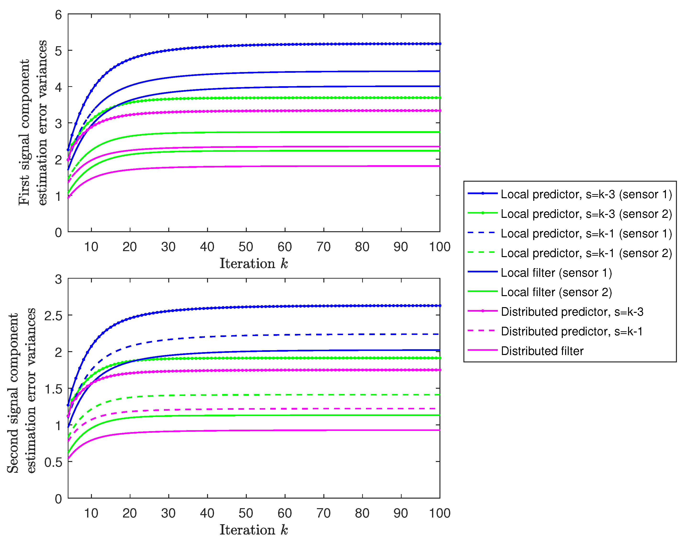
Performance of the local and distributed estimators. Figure 2 illustrates the local and distributed prediction and filtering error variances for $s=k-3,k-1,k,$ of the first and second signal components. For each signal component, this figure shows, on the one hand, that the error variances of the distributed estimators are lower than those of local ones; hence, the distributed fusion estimators provide better estimations of the signal. On the other hand, this figure reveals that the performance of the estimators improves as more observations are used; that is, the error variances of the local and distributed filters are smaller than those of the predictors, and these predictors became more accurate as s increases.

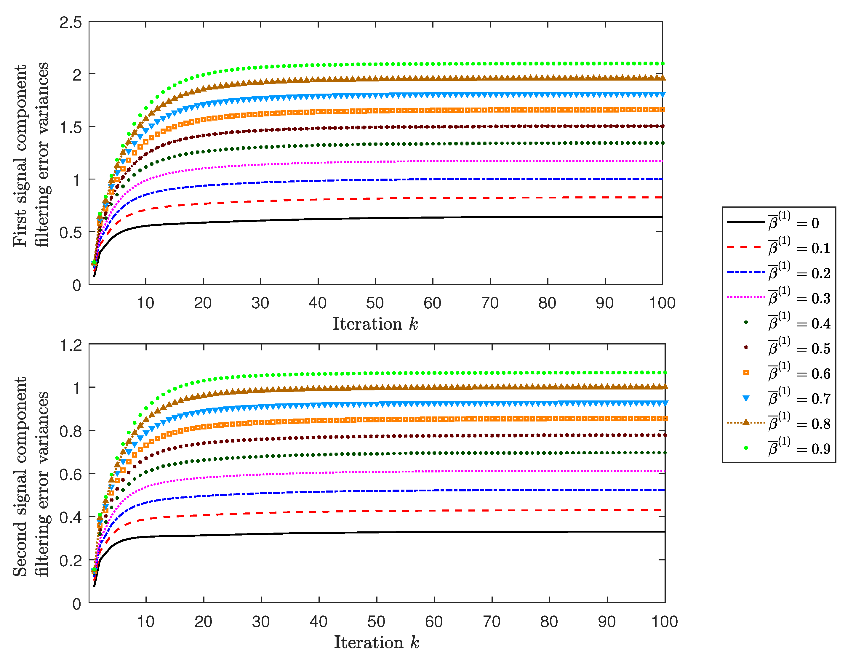
Influence of deception attacks. To analyse the effect of deception attacks, let us assume different values of ${\overline{\beta }}^{\left(1\right)}=0,0.1,\cdots ,0.9$. Figure 3 shows that the distributed filtering error variances for both signal components decrease in line with the probability of success ${\overline{\beta }}^{\left(1\right)}$. Hence, as expected, better estimations of the signal are obtained for lower values of successful attack probability and the best ones are obtained when ${\overline{\beta }}^{\left(1\right)}=0$, since in this case Sensor 1 has not been attacked. A similar analysis for different values of ${\overline{\beta }}^{\left(2\right)}$ as well as for the distributed prediction error variances leads us to the same conclusions.

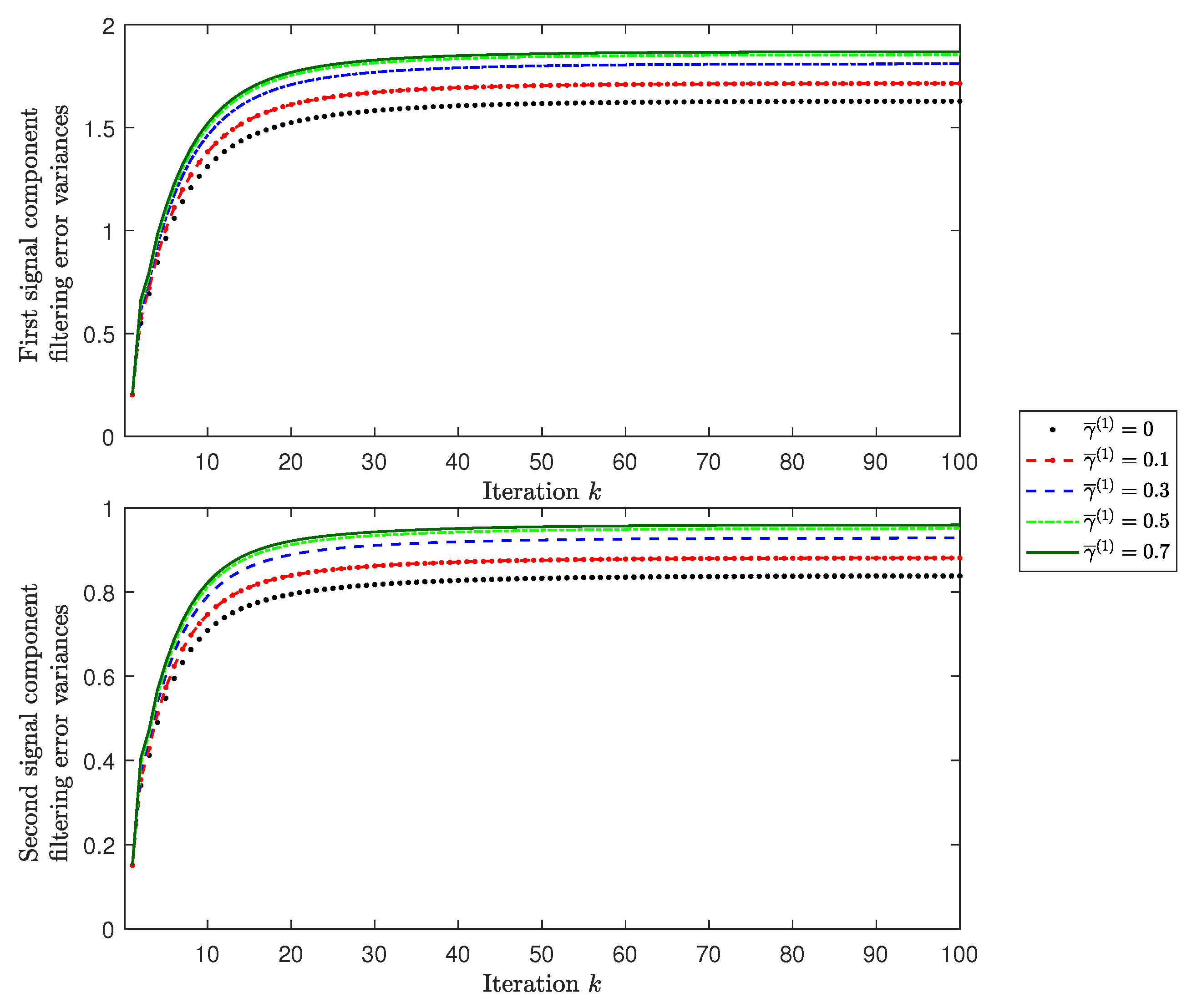
Influence of transmission delays. As in our to analysis of the impact of the deception attack, here we consider that only the delay probabilities for the first sensor change, while the other probabilities remain fixed. Figure 4 shows the distributed filtering error variances when ${\overline{\gamma }}^{\left(1\right)}=0,0.1,0.3,0.5,0.7;$ values greater than 0.7 have not been taken into account since in this case the difference in the results is negligible. From this figure it can be concluded that, as the values of ${\overline{\gamma }}^{\left(1\right)}$ decrease, the distributed filtering error variances become smaller, which means that smaller probabilities of transmission delays provide better results.

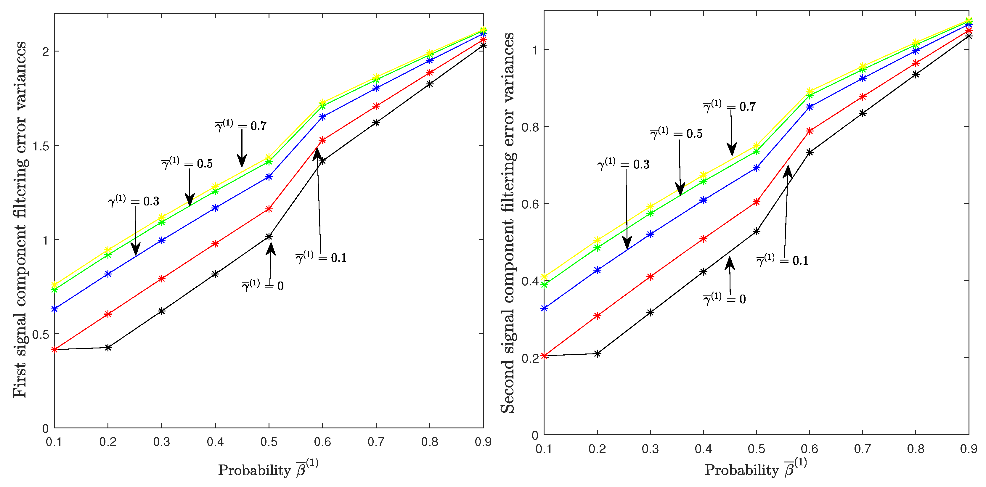
Finally, Figure 5 shows the distributed filtering error variances at $k=55$, varying jointly the different values of ${\overline{\beta }}^{\left(1\right)}$ and ${\overline{\gamma }}^{\left(1\right)}$ previously considered (actually, the results from $k=30$ are very similar, with only negligible variation). In this figure it can be clearly seen that the variances of the filtering error increase with the probability of success of the attacks on the first sensor (${\overline{\beta }}^{\left(1\right)}$) and also with the probability of delay in the measurements from the first sensor (${\overline{\gamma }}^{\left(1\right)}$). Similar results are obtained by varying these probabilities in the second sensor.

5. Conclusions

In this paper, we investigate the distributed fusion linear estimation problem in WSNs that are affected by three types of phenomena that are very common in practical situations, namely deception attacks, correlated noises and delays during transmission. At each sensor, the adversaries may launch random attacks, falsifying the output measurements; these deception attacks are modelled by independent sequences of independent Bernoulli random variables with different and known success probabilities. The measurement noises from different sensors are cross-correlated at the same time step and are also correlated with the signal at the same and subsequent time steps, an assumption that is fulfilled in many practical situations. During the transmission of the sensor outputs through the communication channels to their respective processing centres, these signals can suffer delays, which are modelled by Bernoulli variables describing whether the measures arrive on time or are delayed by one sampling time. For this model, we have derived a distributed fusion prediction and filtering algorithm, using only the information provided by the first and second-order moments of the processes involved in the model; that is, they do not require knowledge of the signal evolution model, although they are also applicable to the classical formulation using this model. In addition, we use a simulation example to show that the estimator accuracy is influenced by the success probabilities of deception attacks and by transmission delays.

Among further research topics of interest in this field, we investigate the stability property in the framework of estimation algorithms using covariance information, and address the problem of the vulnerability or destabilisation of systems subject to sensor deception attacks, as recently discussed in [32,33] for stealthy attacks.

Finally, it would also be of interest to design distributed fusion estimation algorithms in energy-efficient wireless sensor networks whilst considering some of the alternatives that have generated great interest in recent years; for example, event-triggered strategies [34] or other energy-efficient sensor transmission schemes, such as those described in [35].

References

- Ding, D.; Wang, Z.; Shen, B. Recent advances on distributed filtering for stochastic systems over sensor networks. Int. J. Gen. Syst. 2014, 43, 372–386. [Google Scholar] [CrossRef]
- Dong, H.; Wang, Z.; Ding, S.X.; Gao, H. A Survey on Distributed Diltering and Fault Detection for Sensor Networks. Math. Probl. Eng. 2014, 2014, 858624. [Google Scholar] [CrossRef] [Green Version]
- Li, W.; Wang, Z.; Wei, G.; Ma, L.; Hu, J.; Ding, D. A Survey on Multisensor Fusion and Consensus Filtering for Sensor Networks. Discrete Dyn. Nat. Soc. 2015, 2015, 683701. [Google Scholar] [CrossRef] [Green Version]
- Sun, S.L.; Lin, H.; Ma, J.; Li, X. Multi-sensor distributed fusion estimation with applications in networked systems: A review paper. Inf. Fusion. 2017, 38, 122–134. [Google Scholar] [CrossRef]
- Yang, C.; Yang, Z.; Deng, Z. Robust weighted state fusion Kalman estimators for networked systems with mixed uncertainties. Inf. Fus. 2019, 45, 246–265. [Google Scholar] [CrossRef]
- Xia, J.; Gao, S.; Qi, X.; Zhang, J.; Li, G. Distributed cubature H-infinity information filtering for target tracking against uncertain noise statistics. Signal Proccess. 2020, 177, 107725. [Google Scholar] [CrossRef]
- Hu, Z.; Hu, J.; Yang, G. A survey on distributed filtering, estimation and fusion for nonlinear systems with communication constraints: New advances and prospects. Syst. Sci. Control Eng. 2020, 8, 189–205. [Google Scholar] [CrossRef] [Green Version]
- Chen, W.; Ding, D.; Dong, H.; Wei, G. Distributed Resilient Filtering for Power Systems Subject to Denial-of-Service Attacks. IEEE Trans. Syst. Man Cybern. Syst. 2019, 49, 1688–1697. [Google Scholar] [CrossRef]
- Xu, M.; Zhang, Y.; Zhang, D.; Chen, B. Distributed Robust Dimensionality Reduction Fusion Estimation under DoS Attacks and Uncertain Covariances. IEEE Access. 2021, 9, 10328–10337. [Google Scholar] [CrossRef]
- Chen, B.; Ho, D.; Hu, G.; Yu, L. Secure Fusion Estimation for Bandwidth Constrained Cyber-Physical Systems under Replay Attacks. IEEE Trans. Cybern. 2018, 48, 1862–1876. [Google Scholar] [CrossRef]
- Ding, D.; Wang, Z.; Ho, D.; Wei, G. Distributed recursive filtering for stochastic systems under uniform quantizations and deception attacks through sensor networks. Automatica 2017, 78, 231–240. [Google Scholar] [CrossRef]
- Ma, L.; Wang, Z.; Han, Q.-L.; Lam, H.-K. Variance Constrained Distributed Filtering for Time-Varying Systems with Multiplicative Noises and Deception Attacks over Sensor Networks. IEEE Sens. J. 2017, 17, 2279–2288. [Google Scholar] [CrossRef] [Green Version]
- Han, F.; Dong, H.; Wang, Z.; Li, G. Local design of distributed H∞-consensus filtering over sensor networks under multiplicative noises and deception attacks. Int. J. Robust Nonlinear Control. 2019, 29, 2296–2314. [Google Scholar] [CrossRef]
- Caballero-Águila, R.; Hermoso-Carazo, A.; Linares-Pérez, J. Covariance-Based Estimation for Clustered Sensor Networks subject to Random Deception Attacks. Sensors 2019, 19, 3112. [Google Scholar] [CrossRef] [Green Version]
- Feng, J.; Zeng, M. Descriptor recursive estimation for multiple sensors with different delay rates. Int. J. Control. 2011, 84, 584–596. [Google Scholar] [CrossRef]
- Li, N.; Sun, S.; Ma, J. Multi-sensor distributed fusion filtering for networked systems with different delay and loss rates. Digit. Signal Process. 2014, 34, 29–38. [Google Scholar] [CrossRef]
- Chen, B.; Zhang, W.; Yu, L. Distributed Fusion Estimation with Missing Measurements, Random Transmission Delays and Packet Dropouts. IEEE Trans. Automat. Control. 2014, 59, 1961–1967. [Google Scholar] [CrossRef]
- Ma, J.; Sun, S. Distributed fusion filter for networked stochastic uncertain systems with transmission delays and packet dropouts. Signal Process. 2017, 130, 268–278. [Google Scholar] [CrossRef]
- Caballero-Águila, R.; Hermoso-Carazo, A.; Linares-Pérez, J. Networked Fusion Filtering from Outputs with Stochastic Uncertainties and Correlated Random Transmission Delays. Sensors 2016, 16, 847. [Google Scholar] [CrossRef] [Green Version]
- Caballero-Águila, R.; Hermoso-Carazo, A.; Linares-Pérez, J. Fusion Estimation from Multisensor Observations with Multiplicative Noises and Correlated Random Delays in Transmission. Mathematics 2017, 5, 45. [Google Scholar] [CrossRef]
- García-Ligero, M.J.; Hermoso-Carazo, A.; Linares-Pérez, J. Distributed and centralized fusion estimation from multiple sensors with Markovian delays. Appl. Math. Comput. 2012, 219, 2932–2948. [Google Scholar] [CrossRef]
- Shang, Y. Consensus seeking over Markovian switching networks with time-varying delays and uncertain topologies. Appl. Math. Comput. 2016, 273, 1234–1245. [Google Scholar] [CrossRef]
- García-Ligero, M.J.; Hermoso-Carazo, A.; Linares-Pérez, J. Distributed Fusion Estimation with Sensor Gain Degradation and Markovian Delays. Mathematics 2020, 8, 1948. [Google Scholar] [CrossRef]
- Li, X.; Zhu, Y.; Wang, J.; Han, C. Optimal Linear Estimation Fusion—Part I: Unified Fusion Rules. IEEE Trans. Inf. Theory 2003, 49, 2192–2208. [Google Scholar] [CrossRef]
- Yan, L.; Li, X.; Xia, Y.; Fu, M. Optimal sequential and distributed fusion for state estimation in cross-correlated noise. Automatica 2013, 49, 3607–3612. [Google Scholar] [CrossRef]
- Lin, H.; Sun, S. Globally optimal sequential and distributed fusion state estimation for multi-sensor systems with cross-correlated noises. Automatica 2019, 101, 128–137. [Google Scholar] [CrossRef]
- Feng, J.; Wang, Z.; Zeng, M. Distributed weighted robust Kalman filter fusion for uncertain systems with autocorrelated and cross-correlated noises. Inf. Fus. 2013, 14, 78–86. [Google Scholar] [CrossRef]
- Caballero-Águila, R.; Hermoso-Carazo, A.; Linares-Pérez, J.; Wang, Z. A new approach to distributed fusion filtering for networked systems with random parameter matrices and correlated noises. Inf. Fus. 2019, 45, 324–332. [Google Scholar] [CrossRef]
- Wang, D.; Wang, Z.; Shen, B.; Alsaadi, F. Security-guaranteed filtering for discrete-time stochastic delayed systems with randomly occurring sensor saturations and deception attacks. Int. J. Robust Nonlinear Control 2017, 27, 1194–1208. [Google Scholar] [CrossRef] [Green Version]
- Zhang, D.; Xie, J.; Ning, B. Network-based filtering for positive systems with random communication delays and deception attacks. Neurocomputing 2020, 400, 450–457. [Google Scholar] [CrossRef]
- Caballero-Águila, R.; Hermoso-Carazo, A.; Linares-Pérez, J. A Two-Phase Distributed Filtering Algorithm for Networked Uncertain with Fading Measuremente under Deception Attacks. Sensors 2020, 20, 6445. [Google Scholar] [CrossRef] [PubMed]
- Sui, T.; Mo, Y.; Marelli, D.; Sun, X.; Fu, M. The Vulnerability of Cyber-Physical System Under Stealthy Attacks. IEEE Trans. Automat. Control 2021, 66, 637–650. [Google Scholar] [CrossRef] [Green Version]
- Sui, T.; Sun, X. The vulnerability of distributed state estimator under stealthy attacks. Autoatica 2021, 133, 1–12. [Google Scholar] [CrossRef]
- Jiang, L.; Yan, L.; Xia, Y.; Guo, Q.; Fu, M.; Li, L. Distributed fusion in wireless sensor networks based on a novel event-triggered strategy. J. Franklin Inst. 2019, 356, 10315–10334. [Google Scholar] [CrossRef]
- Sriranga, N.; Nagananda, K.G.; Blum, R.S.; Saucan, A.; Varshney, P.K. Energy-efficient Decision Fusion for Distributed Detection in Wireless Sensor Networks. In Proceedings of the 21st International Conference on Information Fusion (FUSION), Cambrige, UK, 10–13 July 2018; pp. 1541–1547. [Google Scholar] [CrossRef] [Green Version]
Figure 1.
Distributed fusion estimation scheme in WNS with attacks and delays.
Figure 2.
Local and distributed prediction and filtering error variances.
Figure 3.
Distributed filtering error variances for different values of .
Figure 4.
Figure 5.
Distributed filtering error variances for different values at of and .