Inflated Unit-Birnbaum-Saunders Distribution

Abstract

The modeling different data behaviour like the human development index as a function of life expectancy, the water capacity of a reservoir with respect to a certain threshold, or the percentage of death rate of an infant before his or her first birthday, are situations which a researcher can face. It is noteworthy that these problems may have in common data with excessive zeros and ones. Then, it is essential to have flexible and accuracy models to fit data with these features. Given the relevance of data modeling with excessive zeros and ones, in this paper, a mixture of discrete and continuous distributions is proposed for modeling data with these behaviors. Additionally, the Unit-Birnbaum-Saunders distribution is considered with the aim to explain the continuous component of the model and the features of a Bernoulli process. The estimation of the parameters is based on the maximum likelihood method. Observed and expected information matrices are derived, illustrating interesting aspects of the likelihood approach. Finally, with practical applications by using real data we can show the advantage of using our proposal concerning the inflated beta model.

1. Introduction

One of the most used distributions to fit fatigue and life data is the Birnbaum-Saunders (BS) distribution, which was introduced in [1]. The BS distribution has a probability density function (PDF) given by

$$f_T\left(t\right)=\frac{t^{-3/2}(t+\beta )}{2\alpha \sqrt{\beta }}\varphi \left(\frac{1}{\alpha }\left[\sqrt{\frac{t}{\beta }}-\sqrt{\frac{\beta }{t}}\right]\right),t>0,$$

(1)

where $\varphi (·)$ is the PDF of the normal distribution, $\alpha >0$ is a shape parameter and $\beta >0$ is a scale parameter. If T is a random variable with BS distribution, then it is denoted as $T\sim \mathrm{BS}(\alpha ,\beta )$.

The BS distribution has been applied in many areas such as biology, medicine, forestry, environment, among others, and it has been extended to a large number of families of distributions. Díaz-García and Leiva-Sánchez [2] for example, introduced the extension of the BS model in the case of the elliptically symmetric distributions, while the elliptically asymmetric case was studied by Vilca-Labra and Leiva-Sánchez [3]. Another extension was considered by Martínez-Flórez et al. [4], which proposed the exponentiated (commonly known as alpha-power model) BS family of distributions. On the other hand, Moreno-Arenas et al. [5] studied the hazard proportional BS model, and Lemonte [6] proposed the multivariate Birnbaum-Saunders model.

Recently, [7] presented a type of BS distribution, which is useful to fit data with support on the interval $(0,1)$, becoming a new alternative to the beta and Kumaraswamy [8] distributions. This new model (named unit-Birnbaum-Saunders (UBS) model) is obtained by applying the transformation $X=exp(-T)$, where $T\sim \mathrm{BS}(\alpha ,\beta )$. Note that, this type of transformation has been used by other authors such as Mazucheli et al. [9], Mazucheli et al. [10] and Menezes et al. [11] among others. It follows that $T=-log\left(X\right)$ with the Jacobian of the transformation obtained by calculating the first derivative of T with respect to X, which is given by $\frac{dt}{dx}=\frac{1}{x}$. Then, by the random variable transformation theorem, see Cassella and Berguer [12] (p. 51), it follows that the PDF of the UBS model is given by

$$\begin{array}{cc}\hfill f_{\mathrm{UBS}}(x;\alpha ,\beta )& =\frac{1}{2x\alpha \beta \sqrt{2\pi }}\left[{\left(-\frac{\beta }{logx}\right)}^{1/2}+{\left(-\frac{\beta }{logx}\right)}^{3/2}\right]\hfill \\ \hfill & \times exp\left\{\frac{1}{2{\alpha }^2}\left[\frac{logx}{\beta }+\frac{\beta }{logx}+2\right]\right\},x\in (0,1),\hfill \end{array}$$

(2)

where $\alpha >0$ is a shape parameter and $\beta >0$ is a scale parameter. The model is denoted as $X\sim \mathrm{UBS}(\alpha ,\beta )$.

Statistical models to explain variables on the unit interval, such as proportions, rates or indexes have been studied by different authors, see [13,14,15,16,17,18,19,20]. Extensions of these models to situations where response variables are on the intervals $[0,1]$, $[0,1)$ or $(0,1]$ have been considered by [21,22,23,24]. Real data applications include the proportion of deaths caused by smoking, problems related to the estimation of the gross domestic product (GDP) and so on. Note that this area has been studied by [9,10,11].

This paper aims to propose an alternative approach for modeling response variables with zero and/or one inflation. A Bernoulli model that links excessive zeros and/or ones with a group of covariates that may influence the probability of their occurrence is considered. One of the main contributions of our proposed model is that it is useful for the analysis of material fatigue data on the interval $[0,1]$ with excess of zeros and/or ones. In the literature, there are other models for fitting data on $[0,1]$ ([22,23,24]), however, these models are not explicitly applied to fitting material fatigue data. We emphasize that the Birnbaum-Saunders distribution is widely used in the analysis of this type of data.

The rest of the paper is organized as follows. In Section 2 the doubly-censored random variable is defined, and the two-part model studied by [25] to analyze this type of variables is presented. Section 3 extends the UBS model to censored data, and the excessive zeros and/or ones are considered by using a mixture of Bernoulli and a doubly-censored UBS model. The parameters estimation is made by using the maximum likelihood approach. The non-singular observed and expected (Fisher) information matrices are derived. Finally, Section 4 presents three analysis with real data sets to compare the proposed model with the modified Beta model.

2. Censoring

A variable is said to be censored when one or more of the observed values are unknown beyond an upper or lower bound. In several practical situations, censoring occurs for limitations of the measuring devices or the experimental project. For example, the needle of a scale that does not provide a reading above 200 kg for all objects that weigh more than this limit, or the measure of viral load in people with HIV. When the data are censored, the probability distribution is a mixture between a continuous and a discrete distribution, and the two-part model by Cragg [25] is a way to analyze situations where data have a mixture between a discrete and a continuous distribution. The two-part model [25] is given by

$$g\left(y_i\right)=p_i(1-I_i)+(1-p_i)f\left(y_i\right)I_i,$$

(3)

where $p_i$ is the probability that determines the relative contribution of the point mass.

The random variable Y is left-censored at the value c, if for a random sample $y_1,\cdots ,y_n$ of size n, only the values of Y that are greater than the constant c can be observed; whereas, for values of Y less than or equal to constant c, only the value c is observed. Therefore, the values of the random variable Y can be written as follows:

$$y_i=\left\{\begin{array}{cc}{y}_i^{\ast },\hfill & \mathrm{if}{y}_i^{\ast }>c,\hfill \\ c,\hfill & \mathrm{if}{y}_i^{\ast }\le c,\hfill \end{array}\right.$$

where c is said to be the censoring point, and the random variable Y has PDF given by

$$g\left(y_i\right)=\left\{\begin{array}{cc}f\left(y_i^{\ast }\right),\hfill & \mathrm{if}{y}_i^{\ast }>c,\hfill \\ p,\hfill & \mathrm{if}{y}_i^{\ast }\le c,\hfill \end{array}\right.$$

For the case $f(·)=\varphi (·)$ it has the Tobit model.

A model is said to be inflated (excess of zeros and/or ones) if the probability mass for some of its points exceeds that allowed by the proposed model. In this case, it is usual to assume that the data distribution is a mixture between a standard distribution and a degenerate distribution concentrated in a point. Some cases that are studied in the statistical literature are the zero-inflated binomial (ZIB) model, zero-inflated Poisson (ZIP) model, and zero-inflated negative binomial (ZINB) model. For more illustration, see [23].

Definition 1.

A random variable Y is said to be a doubly-censored random variable if Y is left-censored and right-censored. For a random sample $y_1^{\ast },y_2^{\ast },\cdots ,y_n^{\ast },$ following certain distribution, it is defined

$$y_i=\left\{\begin{array}{cc}{c}_0,\hfill & if{y}_i^{\ast }\le c_0,\hfill \\ y_i^{\ast },\hfill & if{c}_0<y_i^{\ast }<c_1,\hfill \\ c_1,\hfill & if{y}_i^{\ast }\ge c_1\hfill \end{array}\right.$$

An extension of the model (3) for the doubly-censored case is given by

$$\begin{array}{cc}\hfill g\left(y_i\right)& =p_{0i}{I}_{0i}\left(y_i\right)+p_{1i}{I}_{1i}\left(y_i\right)\hfill \\ \hfill & +(1-p_{0i}-p_{1i})f^{+}\left(y_i\right)(1-I_{0i}\left(y_i\right)-I_{1i}\left(y_i\right)),\hfill \end{array}$$

(4)

where $I_{0i}\left(y_i\right)=1$ if $y_i\le c_0$ and zero otherwise, $I_{1i}\left(y_i\right)=1$ if $y_i>c_1$ and zero otherwise. It has that $p_{0i}$ is the proportion of observations below constant $c_0$ (the lower detection limit) and $p_{1i}$ the proportion of observations above constant $c_1$ (the upper detection limit).

If $y_i^{\ast }\sim \mathrm{N}(\mu ,{\sigma }^2)$, it follows from Definition 1 that the PDF of a doubly-censored random variable Y with normal distribution (DCN), which is an extension of the Tobit model, is given by

$$f\left(y_i\right)=\left\{\begin{array}{cc}\Phi \left(\frac{c_0-\mu }{\sigma }\right),\hfill & \mathrm{if}{y}_i^{\ast }\le c_0,\hfill \\ \frac{1}{\eta }\varphi \left(\frac{y_i-\mu }{\sigma }\right),\hfill & \mathrm{if}{c}_0<y_i^{\ast }<c_1,\hfill \\ 1-\Phi \left(\frac{c_1-\mu }{\sigma }\right),\hfill & \mathrm{if}{y}_i^{\ast }\ge c_1\hfill \end{array}\right.$$

3. The Bernoulli/Doubly Censored Birnbaum—Saunders Mixture Model

In this section, a new doubly-censored model based on unit-Birnbaum-Saunders distribution is introduced.

3.1. Mixture Model

As an alternative to the doubly-censored on $[0,1]$ interval models, the doubly-censored Tobit model, inflated beta distribution and doubly-censored power-normal model; a new model based on a mixture between a Bernoulli random variable and the asymmetric $\mathrm{UBS}(\alpha ,\beta )$ model is introduced. It is considered that the continuous part ranging in $(0,1)$ is modeled by a random variable following a $\mathrm{UBS}(\alpha ,\beta )$ distribution, while the point mass at zero can be modeled by a Bernoulli random variable with parameter $\gamma$, namely $\mathrm{Ber}\left(\gamma \right)$.

Definition 2.

A random variable X that assumes values on the closed interval $[0,1]$ is said to have a zero-and-one-inflated Bernoulli unit-Birnbaum-Saunders distribution (BUBSZOI) with parameters $\alpha ,\beta ,\gamma$ and p, if X has PDF given by

$$f\left(x\right)=\left\{\begin{array}{cc}p(1-\gamma ),\hfill & ifx=0,\hfill \\ (1-p)f_{\mathrm{UBS}}(x;\alpha ,\beta ),\hfill & if0<x<1,\hfill \\ p\gamma ,\hfill & ifx=1,\hfill \end{array}\right.$$

with $0<p,\gamma <1$ and $\alpha ,\beta >0$, where $f_{\mathrm{UBS}}(x_i;\alpha ,\beta )$ is the UBS distribution (2). We write $X\sim \mathrm{BUBSZOI}(\alpha ,\beta ,p,\gamma )$. We can see that, if $X\sim \mathrm{BUBSZOI}(\alpha ,\beta ,p,\gamma )$, then $P(x=0)=p(1-\gamma )$ and $P(x=1)=p\gamma$.

Let $X\sim \mathrm{BUBSZOI}(\alpha ,\beta ,p,\gamma )$, then the cumulative distribution function (CDF) of X is given by

$$\begin{array}{c}\hfill {\mathcal{F}}_X\left(x\right)=\left\{\begin{array}{cc}p(1-\gamma ),\hfill & \mathrm{if}x\le 0,\hfill \\ p(1-\gamma )+(1-p)\Phi \left(w\left(x\right)\right),\hfill & \mathrm{if}0<x<1\hfill \\ 1,\hfill & \mathrm{if}x\ge 1.\hfill \end{array}\right.\end{array}$$

where $w\left(x\right)=\frac{1}{\alpha }\left[\sqrt{\frac{-logx}{\beta }}-\sqrt{\frac{\beta }{-logx}}\right]$. After some algebraic manipulation, the k-th moment of $X\sim \mathrm{BUBSZOI}(\alpha ,\beta ,p,\gamma )$ can be obtained by using

$$\begin{array}{cc}\hfill \mathbb{E}\left(X^k\right)& =p\gamma +(1-p)\frac{2k{\alpha }^2\beta +\sqrt{2k{\alpha }^2\beta +1}+1}{2k{\alpha }^2\beta +1}exp\left[-\frac{\sqrt{2k{\alpha }^2\beta +1}-1}{{\alpha }^2}\right],\hfill \end{array}$$

for $k=1,2,\dots$, it follows that

$$\begin{array}{cc}\hfill {\mu }_1=\mathbb{E}\left(X\right)& =p\gamma +(1-p)\frac{2{\alpha }^2\beta +\sqrt{2{\alpha }^2\beta +1}+1}{2{\alpha }^2\beta +1}exp\left[-\frac{\sqrt{2{\alpha }^2\beta +1}-1}{{\alpha }^2}\right],\hfill \end{array}$$

and

$$\begin{array}{cc}\hfill {\mu }_2=\mathbb{E}\left(X^2\right)& =p\gamma +(1-p)\frac{4{\alpha }^2\beta +\sqrt{4{\alpha }^2\beta +1}+1}{4{\alpha }^2\beta +1}exp\left[-\frac{\sqrt{4{\alpha }^2\beta +1}-1}{{\alpha }^2}\right],\hfill \end{array}$$

so

$$\begin{array}{cc}\hfill Var\left(X\right)& =(1-p){\sigma }_{\mathrm{UBS}}^2+p(1-p){\mu }_1^2+p\gamma \left(1-p\gamma -2(1-p){\mu }_1\right),\hfill \end{array}$$

where ${\sigma }_{\mathrm{UBS}}^2$ is the variance of a random variable following a $\mathrm{UBS}(\alpha ,\beta )$ distribution.

3.1.1. Maximum Likelihood Estimation

Let $\mathbf{X}={(x_1,\dots ,x_n)}^{\top }$ a random sample of a BUBSZOI distribution. Defining ${\sum }_1$ as the sums corresponding to $0<X_i<1$, $n_0={\sum }_{i=1}^n{I}_{\left\{0\right\}}\left(x_i\right),$$n_1={\sum }_{i=1}^n{I}_{\left\{1\right\}}\left(x_i\right)$ and $n_{01}={\sum }_{i=1}^n{I}_{\{0,1\}}\left(x_i\right),$ where $I_A\left(x\right)$ is the indicator function for the set A, then, it follows that the log-likelihood function for the parameter vector $\mathbf{\theta }={(\alpha ,\beta ,p,\gamma )}^{\top }$ given the sample $\mathbf{X}$ can be written as

$$\begin{array}{cc}\hfill \ell (\mathbf{\theta };\mathbf{X})& =n_{01}log\left(p\right)+(n-n_{01})log(1-p)+n_{1}log\left(\gamma \right)+n_{0}log(1-\gamma )\hfill \\ \hfill & +\sum _1\{-log\left(x_i\right)-log\left(\alpha \right)-\frac{1}{2}log\left(\beta \right)+log(-log{x}_i+\beta )\hfill \\ \hfill & -\frac{3}{2}log(-log{x}_i)+\frac{1}{2{\alpha }^2}\left(\frac{log{x}_i}{\beta }+\frac{\beta }{log{x}_i}+2\right)\}.\hfill \end{array}$$

The elements of the score function, defined as the first partial derivative of the log-likelihood function concerning the parameters, are given by

$$\begin{array}{cc}\hfill \frac{\partial \ell (\mathbf{\theta };\mathbf{X})}{\partial \alpha }& =-\frac{1}{\alpha }\sum _1\left[1+\frac{1}{{\alpha }^2}\left(\frac{log{x}_i}{\beta }+\frac{\beta }{log{x}_i}+2\right)\right],\hfill \\ \hfill \frac{\partial \ell (\mathbf{\theta };\mathbf{X})}{\partial \beta }& =-\frac{n}{2\beta }+\sum _1\frac{1}{-log{x}_i+\beta }+\frac{1}{2{\alpha }^2}\sum _1\left(\frac{1}{log{x}_i}-\frac{log{x}_i}{{\beta }^2}\right),\hfill \\ \hfill \frac{\partial \ell (\mathbf{\theta };\mathbf{X})}{\partial p}& =\frac{n_{01}-np}{p(1-p)},\hfill \\ \hfill \frac{\partial \ell (\mathbf{\theta };\mathbf{X})}{\partial \gamma }& =\frac{n_1-\gamma n_{01}}{\gamma (1-\gamma )}\hfill \end{array}$$

The maximum likelihood estimator (MLE) for $\mathbf{\theta }={(\alpha ,\beta ,p,\gamma )}^{\top }$, can be obtained by solving the system of equations that results by equating previous derivatives to zero. Hence, we obtain the solutions $\widehat{p}=n_{01}/n$ and $\widehat{\gamma }=n_1/n_{01}$ for the proportions of zeros and ones, respectively. It can be shown that the estimator $\widehat{p}$ is unbiased for p. The system of equations obtained for ${(\alpha ,\beta )}^{\top }$ does not have an analytical solution and it must be solved by numerical methods like Newton-Raphson or quasi-Newton. The estimator $\widehat{\alpha }$ is obtained as function of $\widehat{\beta }$ by

$$\widehat{\alpha }=\sqrt{\frac{s}{\widehat{\beta }}+\frac{\widehat{\beta }}{r}-2}$$

where $s=\overline{(-logx)}$ and $r={\left(\overline{\left({\left(-logx\right)}^{-1}\right)}\right)}^{-1}$ while $\widehat{\beta }$ is the solution of the equation

$${\beta }^2-(2r+K\left(\beta \right))+r(s+K\left(\beta \right))=0.$$

where $K\left(\beta \right)={\left(\overline{\left({\left(-logx+\beta \right)}^{-1}\right)}\right)}^{-1}.$

3.1.2. Observed Information Matrix

The elements of the observed information matrix are obtained multiplying by minus the second partial derivative of the log-likelihood function concerning each of the parameters, i.e.,

$${\kappa }_{{\theta }_j{\theta }_{j^{\prime }}}=-\frac{{\partial }^2\ell (\mathbf{\theta };\mathbf{X})}{\partial {\theta }_j\partial {\theta }_{j^{\prime }}}$$

where ${\theta }_j,{\theta }_{j^{\prime }}\in {(\alpha ,\beta ,p,\gamma )}^{\top }$. Then, it follows that

$$\begin{array}{cc}\hfill {\kappa }_{\alpha \alpha }& =\sum _1\left[-\frac{1}{{\alpha }^2}+\frac{3}{{\alpha }^2}{a}_{x_i}^2\right],\hfill \\ \hfill {\kappa }_{\beta \alpha }& =\sum _1\frac{1}{{\alpha }^3}\left[\frac{-log{x}_i}{{\beta }^2}-\frac{1}{-log{x}_i}\right],\hfill \\ \hfill {\kappa }_{\beta \beta }& =\sum _1\left[-\frac{1}{2{\beta }^2}+\frac{1}{{(-log{x}_i+\beta )}^2}+\frac{1}{{\alpha }^2{\beta }^3}(-log{x}_i)\right],\hfill \\ \hfill {\kappa }_{pp}& =\frac{n_{01}(1-2p)+n{p}^2}{p^2{(1-p)}^2},\hfill \\ \hfill {\kappa }_{\gamma \gamma }& =\frac{n_1(1-2\gamma )+n_{01}{\gamma }^2}{{\gamma }^2{(1-\gamma )}^2},\hfill \end{array}$$

and

$$\begin{array}{c}\hfill {\kappa }_{\alpha p}=j_{\beta p}=j_{\alpha \gamma }=j_{\beta \gamma }=j_{\gamma p}=0,\end{array}$$

where

$$a_x=\frac{1}{\alpha }\left[\sqrt{\frac{-logx}{\beta }}-\sqrt{\frac{\beta }{-logx}}\right].$$

The elements of the Fisher information matrix can be obtained by multiplying by $n^{-1}$ the expected values of the elements of the matrix of second derivatives of the log-likelihood function. Following [22] the Fisher information matrix for $\mathbf{\theta }={(\alpha ,\beta ,p,\gamma )}^{\top }$ is given by

$$I\left(\mathbf{\theta }\right)=(1-p)\left(\begin{array}{cccc}\frac{1}{{\alpha }^2}& 0& 0& 0\\ 0& \frac{\sqrt{2\pi }+\alpha q\left(\alpha \right)}{\sqrt{2\pi }{\alpha }^2{\beta }^2}& 0& 0\\ 0& 0& \frac{1}{p{(1-p)}^2}& 0\\ 0& 0& 0& \frac{p}{\gamma (1-\gamma )(1-p)}\end{array}\right),$$

where $q\left(\alpha \right)=\alpha \sqrt{2/\pi }-\pi exp\left(2/{\alpha }^2\right)\mathrm{erf}\left(2/\alpha \right)/2$, where $\mathrm{erf}\left(x\right)=\frac{2}{\sqrt{\pi }}{\int }_x^{\infty }exp(-t^2)dt$ is the error function, see [26]. We can note that the $2\times 2$ superior submatrix of $\mathbf{I}\left(\mathbf{\theta }\right)$ matches with the Fisher information matrix of the UBS distribution. This shows that the parameters vectors ${(\alpha ,\beta )}^{\top }$ and ${(p,\gamma )}^{\top }$ are orthogonal, so that the information matrix is blocked orthogonal and can be written as

$$\mathbf{I}\left(\mathbf{\theta }\right)=\mathrm{Diag}\{I_{\alpha ,\beta },I_{p,\gamma }\},$$

where

$$I_{\alpha ,\beta }=\mathrm{Diag}\left\{\frac{1-p}{{\alpha }^2},\frac{(1-p)\left(\sqrt{2\pi }+\alpha q\left(\alpha \right)\right)}{\sqrt{2\pi }{\alpha }^2{\beta }^2}\right\},$$

and

$$I_{p,\gamma }=\mathrm{Diag}\left\{\frac{1}{p(1-p)},\frac{p}{\gamma (1-\gamma )}\right\}.$$

For large samples, the MLE $\widehat{\mathbf{\theta }}$ of $\mathbf{\theta }$ follows a distribution asymptotically normal, i.e.,

$$\sqrt{(}\widehat{\mathbf{\theta }}-\mathbf{\theta })\stackrel{A}{⟶}{N}_4(\mathbf{0},{\mathbf{I}}^{-1}\left(\mathbf{\theta })\right),$$

resulting that the asymptotic variance ${\Sigma }_{\widehat{\mathbf{\theta }}}$, of the MLE $\widehat{\theta }$ is $n^{-1}$ times the inverse of $\mathbf{I}\left(\mathbf{\theta }\right)$ and given by

$${\Sigma }_{\widehat{\mathbf{\theta }}}=\left(\begin{array}{cccc}\frac{{\alpha }^2}{n(1-p)}& 0& 0& 0\\ 0& \frac{1}{n(1-p)}\frac{\sqrt{2\pi }{\alpha }^2{\beta }^2}{\sqrt{2\pi }+\alpha q\left(\alpha \right)}& 0& 0\\ 0& 0& \frac{p(1-p)}{n}& 0\\ 0& 0& 0& \frac{\gamma (1-\gamma )}{np}\end{array}\right).$$

The approximation ${\mathrm{N}}_4(\mathbf{\theta },{\Sigma }_{\widehat{\mathbf{\theta }}})$ can be used to construct the confidence intervals for ${\theta }_r,$ which are given by the formula

$${\widehat{\mathbf{\theta }}}_r\mp z_{1-\rho /2}\sqrt{\widehat{\sigma }\left({\widehat{\mathbf{\theta }}}_r\right)},$$

where $\widehat{\sigma }(·)$ is the r-th diagonal element of the matrix ${\Sigma }_{\widehat{\mathbf{\theta }}}$ and $z_{1-\rho /2}$ is the $100(1-\rho /2)\%$ quantile of the standard normal distribution.

3.2. Mixture Under Reparameterization

A representation of the Bernoulli/UBS mixture model in the form of the doubly-censored model given in (4), that is, it could be written based on the probabilities of the limit points $c_0=0$ and $c_1=1$, call them ${\delta }_0$ and ${\delta }_1>0$ respectively, can be obtained under the reparameterization used by [23] by letting ${\delta }_1=p\gamma$ and ${\delta }_0=1-{\delta }_1$, where ${\delta }_0=P(x=0)$ and ${\delta }_1=P(x=1)$ with $0<{\delta }_0+{\delta }_1<1$, which leads to the PDF given by

$$f\left(x\right)=\left\{\begin{array}{cc}{\delta }_0,\hfill & \mathrm{if}x=0,\hfill \\ (1-{\delta }_0-{\delta }_1)g_{\mathrm{UBS}}(x;\alpha ,\beta ),\hfill & \mathrm{if}0<x<1,\hfill \\ {\delta }_1,\hfill & \mathrm{if}x=1,\hfill \end{array}\right.$$

which is denoted by ${\mathrm{BUBSZOI}}_R(\alpha ,\beta ,{\delta }_0,{\delta }_1)$. If $X\sim {\mathrm{BUBSZOI}}_R(\alpha ,\beta ,{\delta }_0,{\delta }_1)$, then the CDF of X is given by

$${\mathcal{F}}_R\left(x\right)=\left\{\begin{array}{cc}{\delta }_0,\hfill & \mathrm{if}x\le 0,\hfill \\ {\delta }_0+(1-{\delta }_0-{\delta }_1)\Phi \left(w\left(x\right)\right),\hfill & \mathrm{if}0<x<1,\hfill \\ 1,\hfill & \mathrm{if}x\ge 1.\hfill \end{array}\right.$$

where $w\left(x\right)=\frac{1}{\alpha }\left[\sqrt{\frac{-logx}{\beta }}-\sqrt{\frac{\beta }{-logx}}\right]$.

Given a random sample of size n of a $X\sim {\mathrm{BUBSZOI}}_R(\alpha ,\beta ,{\delta }_0,{\delta }_1)$, the log-likelihood function to estimate the parameter vector $\mathbf{\theta }={(\alpha ,\beta ,{\delta }_0,{\delta }_1)}^{\top }$ can be written as

$$\begin{array}{cc}\hfill \ell (\mathbf{\theta };\mathbf{X})& =n_{0}log\left({\delta }_0\right)+n_{1}log\left({\delta }_1\right)+(n-n_{01})log(1-{\delta }_0-{\delta }_1)\hfill \\ \hfill & +\sum _1\{-log\left(x_i\right)-log\left(\alpha \right)-\frac{1}{2}log\left(\beta \right)+log(-log{x}_i+\beta )\hfill \\ \hfill & -\frac{3}{2}log(-log{x}_i)+\frac{1}{2{\alpha }^2}\left(\frac{log{x}_i}{\beta }+\frac{\beta }{log{x}_i}+2\right)\},\hfill \end{array}$$

Then, the score equations follow by equating to zero the score functions, and leading to the following equations

$$\begin{array}{cc}\hfill & -\frac{1}{\alpha }\sum _1\left[1+\frac{1}{{\alpha }^2}\left(\frac{log{x}_i}{\beta }+\frac{\beta }{log{x}_i}+2\right)\right]=0,\hfill \\ \hfill & -\frac{n}{2\beta }+\sum _1\frac{1}{-log{x}_i+\beta }+\frac{1}{2{\alpha }^2}\sum _1\left(\frac{1}{log{x}_i}-\frac{log{x}_i}{{\beta }^2}\right)=0,\hfill \end{array}$$

which can be solved numerically by using Newton-Raphson. From equations $\frac{\partial \ell (\mathbf{\theta };\mathbf{X})}{\partial {\delta }_0}=0$ and $\frac{\partial \ell (\mathbf{\theta };\mathbf{X})}{\partial {\delta }_1}=0$ it is obtained the estimator ${\widehat{\delta }}_0=n_0/n$ of the proportion of zeros in the sample and ${\widehat{\delta }}_1=n_1/n$, the proportions of ones in the sample. In this new model, the Fisher information matrix can be written as $\mathbf{I}\left(\mathbf{\theta }\right)=\mathrm{Diag}\{I_{{\delta }_0,{\delta }_1},I_{\alpha ,\beta }\},$ where the elements of $I_{{\delta }_0,{\delta }_1}$ are given by $i_{{\delta }_0{\delta }_0}=\frac{1-{\delta }_1}{{\delta }_0(1-{\delta }_0-{\delta }_1)},$ $i_{{\delta }_1{\delta }_0}=\frac{1}{1-{\delta }_0-{\delta }_1}$ and $i_{{\delta }_1{\delta }_1}=\frac{1-{\delta }_0}{{\delta }_1(1-{\delta }_0-{\delta }_1)},$ with $I_{\alpha ,\beta }$ as were computed for the model $\mathrm{BUBSZOI}(\alpha ,\beta ,p,\gamma )$.

For this new parameterization, the parameters of the censored and non-censored parts of the model are orthogonal, so the corresponding MLEs are asymptotically orthogonal and the parameters can be estimated separately.

For n large,

$$\sqrt{n}(\widehat{\mathbf{\theta }}-\mathbf{\theta })\stackrel{A}{⟶}{\mathrm{N}}_4(\mathbf{0},{\Sigma }_{\widehat{\mathbf{\theta }}}),$$

meaning that $\widehat{\mathbf{\theta }}$ is consistent and asymptotically normally distributed with sample variance

$${\Sigma }_{\widehat{\mathbf{\theta }}}=\left(\begin{array}{cccc}\frac{{\alpha }^2}{n(1-{\delta }_0-{\delta }_1)}& 0& 0& 0\\ 0& \frac{1}{n(1-{\delta }_0-{\delta }_1)}\frac{\sqrt{2\pi }{\alpha }^2{\beta }^2}{\sqrt{2\pi }+\alpha q\left(\alpha \right)}& 0& 0\\ 0& 0& \frac{{\delta }_0(1-{\delta }_0)}{n}& -\frac{{\delta }_0{\delta }_1}{n}\\ 0& 0& -\frac{{\delta }_0{\delta }_1}{n}& \frac{{\delta }_1(1-{\delta }_1)}{n}\end{array}\right).$$

3.3. Censored Models for Zero or One Inflation

Particular cases of the previous zero-and-one-inflated model, are the situation of zero-inflated and one-inflated. In the case of the zero-inflated, the density function is given by:

$$f\left(x\right)=\left\{\begin{array}{cc}{\delta }_0,\hfill & \mathrm{if}x=0,\hfill \\ (1-{\delta }_0)g_{\mathrm{UBS}}(x;\alpha ,\beta ),\hfill & \mathrm{if}0<x<1.\hfill \end{array}\right.$$

where $0<{\delta }_0=P(x=0)<1$. This model is denoted ${\mathrm{BUBSZI}}_R(\alpha ,\beta ,{\delta }_0)$. The log-likelihood function of $\mathbf{\theta }={(\alpha ,\beta ,{\delta }_0)}^{\top }$ can be written as:

$$\begin{array}{cc}\hfill \ell (\mathbf{\theta };\mathbf{X})& =n_{0}log\left({\delta }_0\right)+(n-n_0)log(1-{\delta }_0)\hfill \\ \hfill & +\sum _1\{-log\left(x_i\right)-log\left(\alpha \right)-\frac{1}{2}log\left(\beta \right)+log(-log{x}_i+\beta )\hfill \\ \hfill & -\frac{3}{2}log(-log{x}_i)+\frac{1}{2{\alpha }^2}\left(\frac{log{x}_i}{\beta }+\frac{\beta }{log{x}_i}+2\right)\},\hfill \end{array}$$

The MLEs of the parameters $\alpha$ and $\beta$ are obtained numerically from the equations $\frac{\partial \ell (\mathbf{\theta };\mathbf{X})}{\partial \alpha }=0$ and $\frac{\partial \ell (\mathbf{\theta };\mathbf{X})}{\partial \beta }=0$, as in the general case of the model ${\mathrm{BUBSZOI}}_R(\alpha ,\beta ,{\delta }_0,{\delta }_1)$. For the case of the parameter ${\delta }_0$, the estimate is obtained from the equation $\frac{\partial \ell (\mathbf{\theta };\mathbf{X})}{\partial {\delta }_0}=0$ and it is given by ${\widehat{\delta }}_0=n_0/n$, which is the estimated proportion of zeros in the sample.

The variance of the MLE vector $\theta ={(\alpha ,\beta ,{\delta }_0)}^{\top }$ takes the form

$${\Sigma }_{\widehat{\mathbf{\theta }}}=\left(\begin{array}{ccc}\frac{{\alpha }^2}{n(1-{\delta }_0)}& 0& 0\\ 0& \frac{1}{n(1-{\delta }_0)}\frac{\sqrt{2\pi }{\alpha }^2{\beta }^2}{\sqrt{2\pi }+\alpha q\left(\alpha \right)}& 0\\ 0& 0& \frac{{\delta }_0(1-{\delta }_0)}{n}\end{array}\right).$$

In the case of the one-inflated, the likelihood function is given by:

$$f\left(x\right)=\left\{\begin{array}{cc}{\delta }_1,\hfill & \mathrm{if}x=1,\hfill \\ (1-{\delta }_1)g_{\mathrm{UBS}}(x;\alpha ,\beta ),\hfill & \mathrm{if}0<x<1.\hfill \end{array}\right.$$

where $0<{\delta }_1=\mathrm{Pr}(x=1)<1$. This is denoted by ${\mathrm{BUBSOI}}_R(\alpha ,\beta ,{\delta }_1)$. The log-likelihood function of $\mathbf{\theta }={(\alpha ,\beta ,{\delta }_1)}^{\top }$ can be written as

$$\begin{array}{cc}\hfill \ell (\mathbf{\theta };\mathbf{X})& =n_{1}log\left({\delta }_1\right)+(n-n_1)log(1-{\delta }_1)\hfill \\ \hfill & +\sum _1\{-log\left(x_i\right)-log\left(\alpha \right)-\frac{1}{2}log\left(\beta \right)+log(-log{x}_i+\beta )\hfill \\ \hfill & -\frac{3}{2}log(-log{x}_i)+\frac{1}{2{\alpha }^2}\left(\frac{log{x}_i}{\beta }+\frac{\beta }{log{x}_i}+2\right)\},\hfill \end{array}$$

As in the case of the zero-inflated, the MLEs of the parameters $\alpha$ and $\beta$ are obtained numerically from the equations $\frac{\partial \ell (\mathbf{\theta };\mathbf{X})}{\partial \alpha }=0$ and $\frac{\partial \ell (\mathbf{\theta };\mathbf{X})}{\partial \beta }=0,$ while ${\delta }_1$ is estimated from equation $\frac{\partial \ell (\mathbf{\theta };\mathbf{X})}{\partial {\delta }_1}=0$, thus, it is obtained the estimator ${\widehat{\delta }}_1=n_1/n$, which is the proportion of ones in the sample.

The variance of the MLE of the parameter vector $\mathbf{\theta }={(\alpha ,\beta ,{\delta }_1)}^{\top }$, is

$${\Sigma }_{\widehat{\mathbf{\theta }}}=\left(\begin{array}{ccc}\frac{{\alpha }^2}{n(1-{\delta }_1)}& 0& 0\\ 0& \frac{1}{n(1-{\delta }_1)}\frac{\sqrt{2\pi }{\alpha }^2{\beta }^2}{\sqrt{2\pi }+\alpha q\left(\alpha \right)}& 0\\ 0& 0& \frac{{\delta }_1(1-{\delta }_1)}{n}\end{array}\right).$$

3.4. Testing Nested Models

Let consider $F_{\theta }$ and $G_{\gamma }$ with corresponding density functions $f(y_i\mid x_i,\theta )$ and $g(y_i\mid x_i,\beta )$, respectively, the likelihood ratio statistic to compare models is given by

$$LR(\widehat{\mathbf{\theta }},\widehat{\mathbf{\beta }})\equiv {\ell }_f\left(\widehat{\mathbf{\theta }}\right)-{\ell }_g\left(\widehat{\mathbf{\beta }}\right)=\sum _{i=1}^{n}log\frac{f(y_i\mid {\mathbf{x}}_i,\widehat{\mathbf{\theta }})}{g(y_i\mid {\mathbf{x}}_i,\widehat{\mathbf{\beta }})},$$

This likelihood ratio statistic does not have a chi-square distribution. To overcome this problem, Vuong [27] proposed an alternative approach based on the Kullback-Liebler information criterion, [28]. The statistic is given by

$$T_{\mathrm{LR},\mathrm{NN}}=\frac{1}{\sqrt{n}}\frac{LR(\widehat{\mathbf{\theta }},\widehat{\mathbf{\beta }})}{{\widehat{\omega }}^2},$$

where

$$\begin{array}{cc}\hfill {\widehat{\omega }}^2& =\frac{1}{n}\sum _{i=1}^n{\left(log\frac{f(y_i\mid {\mathbf{x}}_i,\widehat{\mathbf{\theta }})}{g(y_i\mid {\mathbf{x}}_i,\widehat{\mathbf{\beta }})}\right)}^2-{\left(\frac{1}{n}\sum _{i=1}^n\left(log\frac{f(y_i\mid {\mathbf{x}}_i,\widehat{\mathbf{\theta }})}{g(y_i\mid {\mathbf{x}}_i,\widehat{\mathbf{\beta }})}\right)\right)}^2\hfill \end{array}$$

is an estimator for the variance of $\frac{1}{\sqrt{n}}LR(\widehat{\mathbf{\theta }},\widehat{\mathbf{\beta }})$.

Hence, it was shown that, as $n\to \infty$,

$$T_{\mathrm{LR},\mathrm{NN}}\stackrel{d}{⟶}\mathrm{N}(0,1)$$

under

$$H_0:E\left[log\frac{f(y_i\mid {\mathbf{x}}_i,\mathbf{\theta })}{g(y_i\mid {\mathbf{x}}_i,\mathbf{\beta })}\right]=0,$$

then, the models are equivalent. At the 5% level, being $z_{0.025}$ the critical value, the model is rejected if $T_{\mathrm{LR},\mathrm{NN}}>z_{0.025}$, that is, $T_{\mathrm{LR},\mathrm{NN}}<-z_{0.025}$.

4. Real Data Illustrations

In this section, the usefulness of the proposed models is presented. The BUBSZOI and BUBSZI distributions are fitted to real data sets.

4.1. Illustration 1 of the BUBSZOI Model

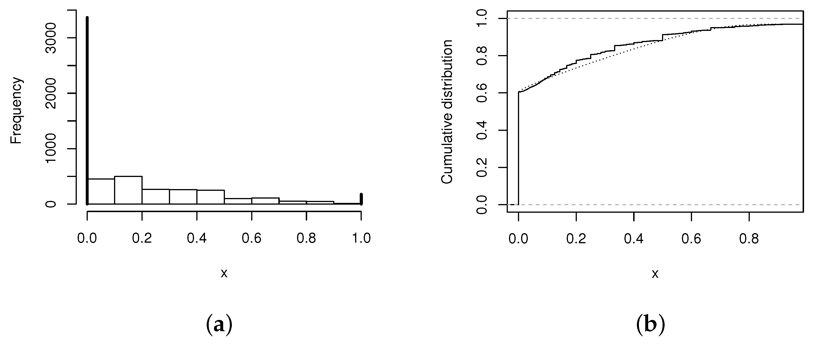
For this illustration, we use the data set available at http:www.datasus.gov.br, (accesed date: 27 November 2021). This data set corresponds to the proportions of infant deaths in 5561 Brazilian counties. The histogram, that show the behavior of the data, is given in the following Figure 1 (on left).

Table 1. Statistical summary of the infant deaths data.

Data	n	Mean	SE	Bias	Kurtosis
Complete	5561	0.137	0.246	2.069	6.647
Non-censored	3541	0.292	0.216	0.811	2.94

shows some descriptive statistics of the data set. For this data set, the inflated beta (BEINF) distribution was fitted, Ref. [23]. In addition, the MBLPN model proposed by [22] is fitted, where is assumed a mixture of a Bernoulli random variable for the discrete part, and a log-power-normal model for the continuous part (between zero and one). This is denoted by $\mathrm{MBLPN}(\mu ,\sigma ,\alpha ,{\delta }_0,{\delta }_1)$. The BUBSZOI model is also fitted. The MLEs (with standard errors in parentheses) of the fitted parameter models are given in

Table 2. The MLE of the parameters of the mixtures of the Bernoulli distribution with: Beta, LPN and UBS models.

Est.	BEINF	MBLPN	BUBSZOI
$\widehat{\mu }$	0.297 (0.004)	0.661 (0.0066)	–
$\widehat{\sigma }$	0.456 (0.005)	0.022 (0.0030)	–
$\widehat{\alpha }$	–	0.001 (0.001)	0.783 (0.012)
$\widehat{\beta }$	–	–	1.198 (0.019)
${\widehat{\delta }}_0$	0.606 (0.007)	0.606 (0.007)	0.606 (0.007)
${\widehat{\delta }}_1$	0.031 (0.002)	0.031 (0.002)	0.031 (0.002)

. Figure 1b is the CDF for the BUBSZOI model, showing that the model presents a good fit for the studied data set.

To compare BUBSZOI model against the MBLPN model of [22] and the BEINF model, a test of non-nested models is used. Let $F_{\theta }$ the BUBSZOI model and $G_{\beta },$ the MBLPN model, the Vuong’s approach leads to the observed value $T_{\mathrm{LR},\mathrm{NN}}=-0.0116$ which is not greater than the critical value $z_{0.025}=1.96$ and hence, the MBLPN distribution is not better than the BUBSZOI model. Similarly, to compare the BUBSZOI and BEINF models, it has $T_{\mathrm{LR},\mathrm{NN}}=55.3415$ which is greater than the critical value $z_{0.025}=1.96$ which favors the BUBSZOI model, then the best model to fit the data is the BUBSZOI.

4.2. Illustration of the BUBSZI Model

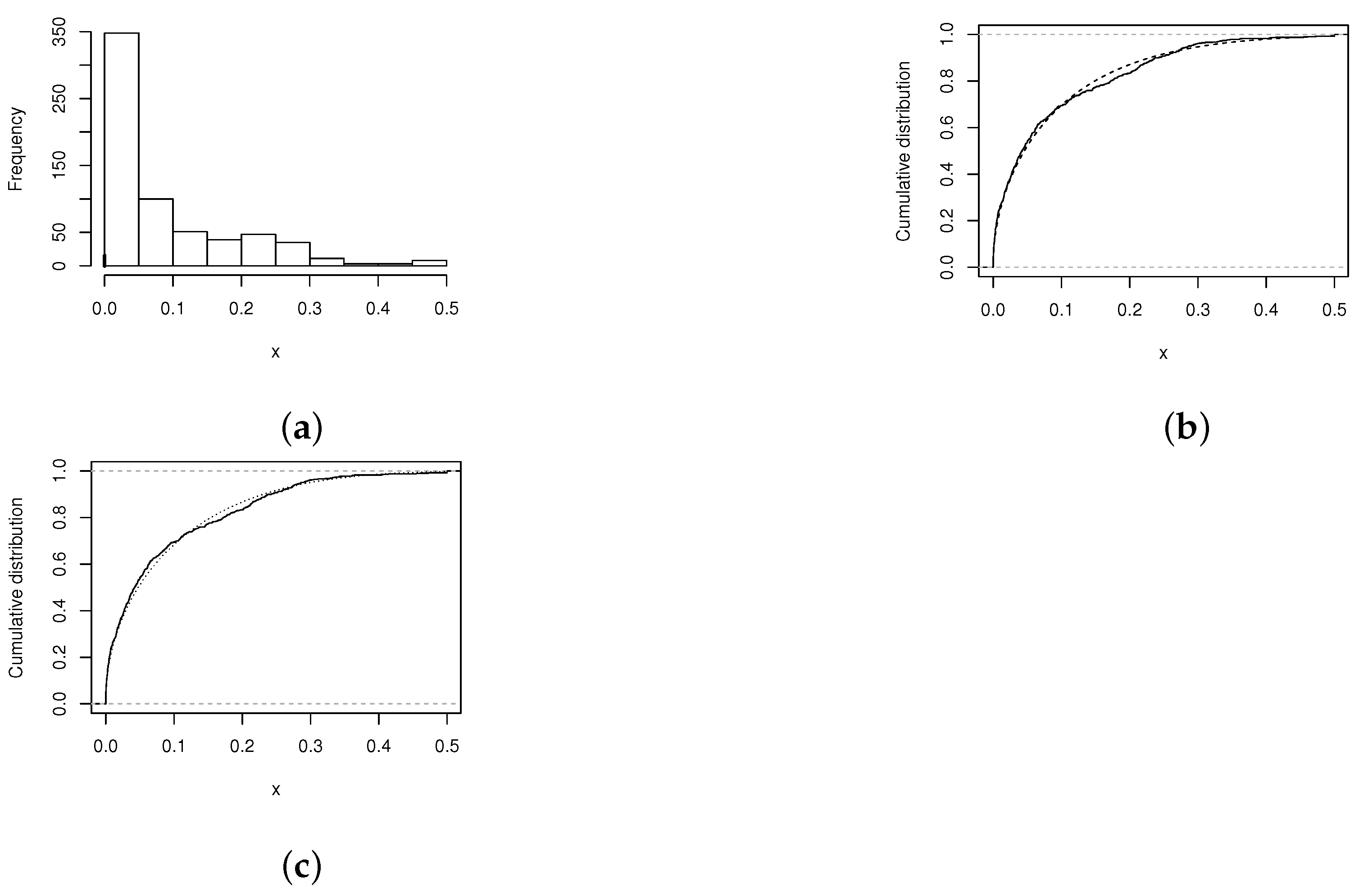
A situation in which our model can be useful, occurs when we want to fit a statistical model to data sets related to percentages of people with some feature of interest (with high or low frequency of occurrence). For example, this second illustration uses the database available and explained in detail at http:www.pnud.org.br (accessed date: 14 September 2021), corresponding to the percentage of people whit certain poverty conditions. Here, the frequency histogram of the data is presented in Figure 2a. Note that their shape is as an inverted J, a feature that can be modeled by the BEZI model, see [23], it is assumed a mixture of a Bernoulli random variable for the discrete part and a beta regression for the continuous (between zero and one), which is denoted by $\mathrm{BEZI}(\mu ,\sigma ,{\delta }_0)$. The total number of zeros in the sample is represented with a vertical bar at zero. Additionally, we consider a left-censored Tobit model and the BUBSZI distribution. The MLEs (with standard errors in parentheses) of the parameters of the proposed models are presented in

Table 3. The MLE of the parameters of the BEZI, Tobit and BUBSZI models.

Est.	BEZI	Tobit	BUBSZI
$\widehat{\mu }$	0.088 (0.004)	0.085 (0.004)	–
$\widehat{\sigma }$	6.290 (0.404)	0.104 (0.003)	–
$\widehat{\alpha }$	–	–	0.575 (0.016)
$\widehat{\beta }$	–	–	2.993 (0.066)
${\widehat{\delta }}_0$	0.023 (0.006)	–	0.023 (0.006)

.

Figure 2 also shows the CDF for the BEZI and BUBSZI model, illustrating the fact that the models present a good fit for the studied data set.

Now, being $F_{\theta }$ the BUBSZI model and $G_{\beta },$ the BEZI model, the Vuong’s approach leads to the observed value $T_{\mathrm{LR},\mathrm{NN}}=18.6431$. This value is greater than the critical point $z_{0.025}=1.96$ and hence, the BUBSZI distribution is the best model. Similarly, for comparing models BUBSZI and Tobit, we have $T_{\mathrm{LR},\mathrm{NN}}=11.5110$ which favors the BUBSZI model, then the best model to fit the data is the BUBSZI model.

4.3. Illustration 2 of the BUBSZOI Model

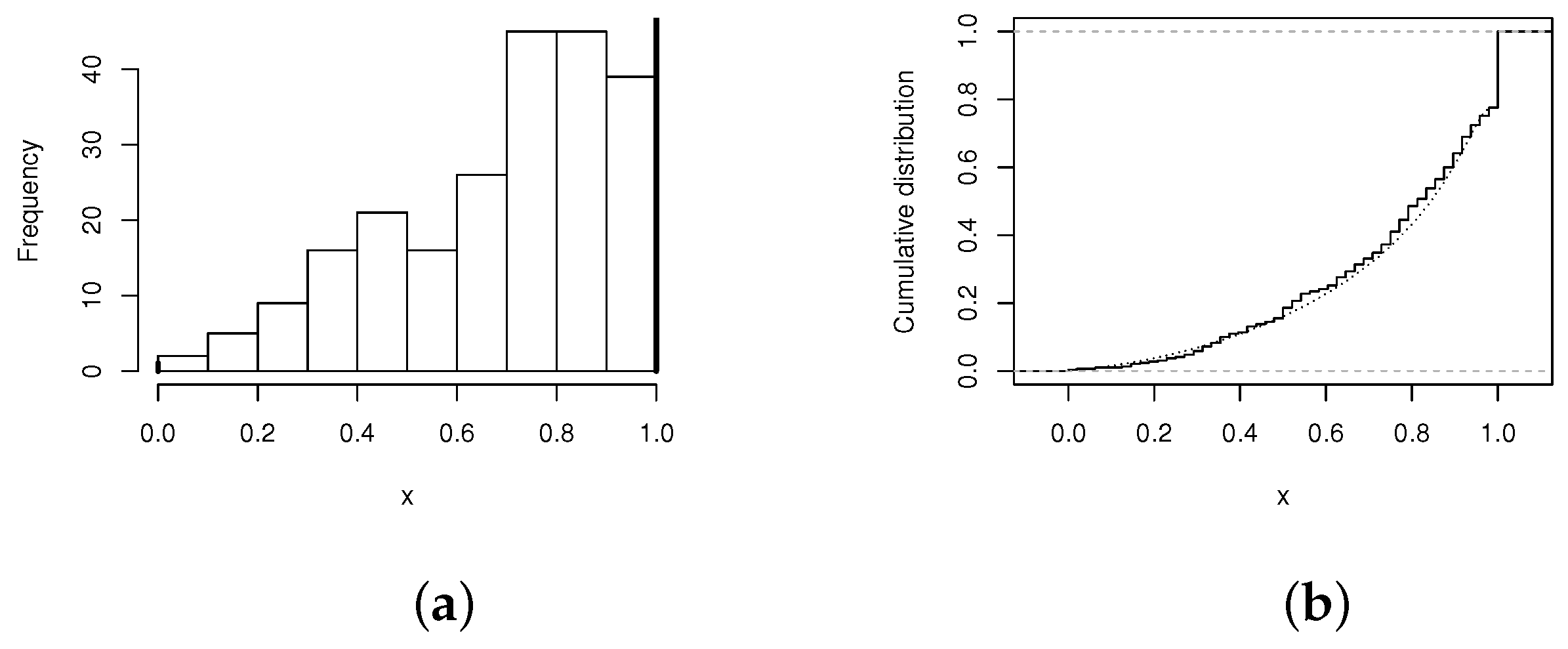
As was mentioned in the introduction, medicine is an important area of application of our model. So, this new illustration is made by using the data set which was studied by [29] and corresponds to a clinical marker of periodontal disease. The histogram of the response $\left(X\right)$ (proportion of diseased tooth sites of the incisors tooth), is presented in Figure 3a showing the data behavior. Notice that, the data set presents high inflation of $X=1$, but for some units, we have $X=0$.

We fit the beta and BUBSZOI models to the data set. The MLEs of the $\mu$ and $\sigma$ of the beta model are given by $\widehat{\mu }=0.6774\left(0.0143\right)$ and $\widehat{\sigma }=0.4698\left(0.0158\right)$, while for the BUBSZOI model, we obtained the MLEs $\widehat{\alpha }=1.2135\left(0.0573\right)$ and $\widehat{\beta }=0.2638\left(0.0178\right)$. The estimates of the ${\delta }_0$ and ${\delta }_1$ in both models are ${\widehat{\delta }}_0=0.0034\left(0.0034\right)$ and ${\widehat{\delta }}_1=0.2241\left(0.0244\right)$.

The value of Vuong’s statistic to compare the models under consideration is given by $T_{\mathrm{LR},\mathrm{NN}}=26.99265$, which is greater than $z_{0.025}=1.96$ which favors the BUBSZOI model, so the best model to fit the data is the BUBSZOI model. Figure 3 (on right), presents the CDF of the BUBSZOI model, illustrating the fact that the model presents a good fit for the studied data set.

5. Concluding Remarks

The modeling of data with excessive zeros or ones is a task that is required in areas like economy, medicine, agriculture, and so on. Possible applications in these areas could be related to the modeling of the infant mortality rate, the proportion of deaths caused by smoking, a clinical marker of periodontal disease, the estimation of the gross domestic product, or the mortality in traffic accidents, among others. As shown in previous sections, different alternatives could be found in the literature to model this behavior, as the extensions of the inflated beta model, which were used to compare their performance with our proposal.

This paper discusses an alternative to the beta regression model in the situation of excessive zeros and/or ones. The approach is based on an extension of the Tobit model with excess of zeros considered in [30]. The estimation is based on the likelihood approach and the Fisher information matrix is derived having orthogonality between the parameters, which simplifies large sample properties of the maximum likelihood estimators. Three illustrations with real data show that the proposed models can be even better than the extensions of the inflated beta model considered in [23].

References

- Birnbaum, Z.W.; Saunders, S.C. A new family of life distributions. J. Appl. Probab. 1969, 6, 319–327. [Google Scholar] [CrossRef]
- Díaz-García, J.A.; Leiva-Sánchez, V. A new family of life distributions based on the elliptically contoured distributions. J. Stat. Plan. Inference 2005, 128, 445–457. [Google Scholar] [CrossRef]
- Vilca-Labra, F.; Leiva-Sánchez, V. A new fatigue life model based on the family of skew-elliptical distributions. Commun. Stat. Theory Methods 2006, 35, 229–244. [Google Scholar] [CrossRef]
- Martínez-Flórez, G.; Bolfarine, H.; Gómez, H.W. An alpha-power extension for the Birnbaum-Saunders distribution. Statistics 2014, 48, 896–912. [Google Scholar] [CrossRef]
- Moreno-Arenas, G.; Martínez-Flórez, G.; Barrera-Causil, C. Proportional hazard Birnbaum-Saunders distribution with application to the survival data analysis. Rev. Colomb. Estadística 2016, 39, 129–147. [Google Scholar] [CrossRef]
- Lemonte, A.J. Multivariate Birnbaum-Saunders regression model. J. Stat. Comput. Simul. 2013, 46, 2244–2257. [Google Scholar] [CrossRef]
- Mazucheli, J.; Menezes, A.F.B.; Dey, S. The unit-Birnbaum-Saunders distribution with applications. Chil. J. Stat. 2018, 9, 47–57. [Google Scholar]
- Kumaraswamy, P. A generalized probability density function for double-bounded random processes. J. Hydrol. 1980, 46, 79–88. [Google Scholar] [CrossRef]
- Mazucheli, J.; Menezes, A.F.B.; Dey, S. Improved maximum-likelihood estimators for the parameters of the unit-gamma distribution. Commun. Stat. Theory Methods 2018, 47, 3767–3778. [Google Scholar] [CrossRef]
- Mazucheli, J.; Menezes, A.F.B.; Ghitany, M.E. The unit-Weibull distribution and associated inference. J. Appl. Probab. Stat. 2018, 13, 1–22. [Google Scholar]
- Menezes, A.F.B.; Mazucheli, J.; Dey, S. The unit-logistic distribution: Different methods of estimation. Pesqui. Oper. 2018, 38, 555–578. [Google Scholar] [CrossRef]
- Cassella, G.; Berger, R.L. Statistical Inference; Duxbury: Belmont, CA, USA, 2002. [Google Scholar]
- Bayes, C.L.; Bazan, J.L.; García, C. A new robust regression model for proportions. Bayesian Anal. 2012, 7, 841–866. [Google Scholar] [CrossRef]
- Branscum, A.J.; Johnson, W.O.; Thurmond, M.C. Bayesian beta regression: Applications to household expenditure data and genetic distance between foot-and-mouth diseases viruses. Aust. N. Z. J. Stat. 2007, 49, 287–301. [Google Scholar] [CrossRef]
- Cribari-Neto, F.; Vasconcellos, K.L.P. Nearly unbiased maximum likelihood estimation for the beta distribution. J. Stat. Comput. Simul. 2002, 72, 107–118. [Google Scholar] [CrossRef]
- Ferrari, S.; Cribari-Neto, F. Beta regression for modelling rates and proportions. J. Appl. Stat. 2004, 31, 799–815. [Google Scholar] [CrossRef]
- Kieschnick, R.; McCullough, B.D. Regression analysis of variates observed on (0, 1): Percentages, proportions and fractions. Stat. Model. 2003, 3, 193–213. [Google Scholar] [CrossRef] [Green Version]
- Lemonte, A.J.; Cribari-Neto, F.; Vasconcellos, K.L.P. Improved statistical inference for the two-parameter Birnbaum-Saunders distribution. Comput. Stat. Data Anal. 2007, 51, 4656–4681. [Google Scholar] [CrossRef]
- Paolino, P. Maximum likelihood estimation of models with beta-distributed dependent variables. Political Anal. 2001, 9, 325–346. [Google Scholar] [CrossRef]
- Vasconcellos, K.L.P.; Cribari-Neto, F. Improved maximum likelihood estimation in a new class of beta regression models. Braz. J. Probab. Stat. 2005, 19, 13–31. [Google Scholar]
- Martínez-Flórez, G.; Bolfarine, H.; Gómez, H.W. Doubly censored power-normal regression models with inflation. Test 2014, 24, 265–286. [Google Scholar] [CrossRef]
- Martínez-Flórez, G.; Bolfarine, H.; Gómez, H.W. Power-models for proportions with zero/one excess. Appl. Math. Inf. Sci. 2018, 24, 293–303. [Google Scholar] [CrossRef]
- Ospina, R.; Ferrari, S.L.P. Inflated beta distribution. Stat. Pap. 2010, 51, 111–126. [Google Scholar] [CrossRef] [Green Version]
- Ospina, R.; Ferrari, S.L.P. A general class of zero-or-one inflated beta regression models. Comput. Stat. Data Anal. 2012, 56, 1609–1623. [Google Scholar] [CrossRef] [Green Version]
- Cragg, J. Some statistical models for limited dependent variables with application to the demand for durable goods. Econometrica 1971, 39, 829–844. [Google Scholar] [CrossRef]
- Prudnikov, A.P.; Brychkov, Y.A.; Marichev, O.I. Inntegrals and Series: More Special Functions; Gordon and Breach Science Publishers: New York, NY, USA, 1990. [Google Scholar]
- Vuong, Q.H. Likelihood ratio tests for model selection and non-nested hypotheses. Econometrica 1989, 57, 307–333. [Google Scholar] [CrossRef] [Green Version]
- Kullback, S.; Leibler, R.A. On information and sufficiencys. Ann. Math. Stat. 1951, 22, 79–86. [Google Scholar] [CrossRef]
- Galvis, D.M.; Lachos, V.H.; Bandyphaday, D. Augmented mixed models for clustered proportion data. Stat. Methods Med. Res. 2017, 26, 880–897. [Google Scholar]
- Moulton, L.H.; Halsey, N.A. A mixture model with detection limits for regression analyses of antibody response to vaccine. Biometrics 1995, 51, 1570–1578. [Google Scholar] [CrossRef]
Figure 1.
(a) Histogram of the death proportions. (b) Graphs: empiric (solid line), BUBSZOI model (dotted line).
Figure 2.
(a) Histogram of the death proportions. (b) Graphs: empiric (solid line), BEZI (dashed line). (c) Graphs: empiric (solid line), BUBSZI (dotted line).
Figure 3.
(a) Histogram of the the variable X. (b) Graphs: empiric (solid line), BUBSZOI (dotted line).