Pathwise Convergent Approximation for the Fractional SDEs

Abstract

Fractional stochastic differential equation (FSDE)-based random processes are used in a wide spectrum of scientific disciplines. However, in the majority of cases, explicit solutions for these FSDEs do not exist and approximation schemes have to be applied. In this paper, we study one-dimensional stochastic differential equations (SDEs) driven by stochastic process with Hölder continuous paths of order $1/2<\gamma <1$. Using the Lamperti transformation, we construct a backward approximation scheme for the transformed SDE. The inverse transformation provides an approximation scheme for the original SDE which converges at the rate $h^{2\gamma }$, where h is a time step size of a uniform partition of the time interval under consideration. This approximation scheme covers wider class of FSDEs and demonstrates higher convergence rate than previous schemes by other authors in the field.

1. Introduction

Stochastic differential equations (SDEs) are used as a modeling tool in many fields of science. Currently, a lot of research is being conducted on models with fractional Brownian motion (fBm) $B^H$, $0<H<1$, since fBm introduces a memory element, which provides new and promising modeling possibilities. It should be noted that the definition of SDEs driven by fBm differs substantially from the definition used by standard Brownian-motion-driven SDEs. Furthermore, there is more than one way to define these SDEs (for example, in our paper, we will use the Riemann–Stieltjes integral to achieve this). The general conditions under which the fractional diffusion process has a unique solution were obtained in [1]. These conditions impose more strict restrictions on the coefficients than in the case of SDEs driven by standard Brownian motion (sBm).

Classical financial models such as Chan–Karoli–Longstaff–Sanders (CKLS), Cox–Ingersoll–Ross (CIR), and Ait–Sahalia are defined using SDEs driven by standard Brownian motion. Replacing the standard Brownian motion with a fractional Brownian motion, we obtain a fractional analogue of these classical models. In many of these models, the solution positivity is a desirable property. The positivity of fractional CIR model was studied in [2,3]. The conditions under which fractional CKLS, Ait–Sahalia and other models have positive solutions follow from [4,5,6]. The above-mentioned financial models have a strictly positive diffusion coefficient.

In this paper, we shall consider a one-dimensional SDE driven by an arbitrary stochastic process $Z={\left(Z_t\right)}_{t⩾0}$, $Z_0=0$, with Hölder continuous paths of order $1/2<\gamma <1$

$$X_t=x_0+{\int }_0^t\alpha \left(X_s\right)ds+{\int }_0^t\sigma \left(X_s\right)d{Z}_s,x_0\in \mathbb{R},t\in [0,T],$$

(1)

where $x_0$ is a constant, and the coefficients $\alpha ,\sigma :\mathbb{R}\to \mathbb{R}$ are continuous functions. The stochastic integral in Equation (1) is a pathwise Riemann–Stieltjes integral, and thus the whole equation is understood as a pathwise Riemann–Stieltjes integral equation (special case $Z=B^H$). The conditions under which the Equation (1) has a unique solution X were obtained in [7].

A lot of SDEs cannot be solved explicitly; thus, it is important to find their approximated solutions by applying some numerical methods. For SDEs driven by sBm, authors usually consider the convergence rate of strong Itô–Taylor approximation schemes of the SDEs solutions. From a strong convergence rate, one can obtain the pathwise convergence rate (see [8,9] and the references therein), which provides the error of the actual approximation.

For Equation (1) with $Z=B^H$ and rather smooth and bounded coefficients $\alpha$ and $\sigma$, different explicit approximation schemes were considered in [10,11,12,13] (see also the references therein). Particularly, in [10,12,13], Euler and other higher-order approximation schemes were considered; [11] presents a new method that converges with weaker conditions compared to the results in [12]; and in [14], less strict conditions for the coefficients were used in the explicit Euler approximation.

The purpose of this work is to obtain an approximation scheme under weaker conditions and of a higher order convergence rate than in the articles mentioned above. For this, we require the diffusion coefficient to be strictly positive, i.e., ${inf}_{x\in \mathbb{R}}\sigma \left(x\right)>0$. Such restriction on a diffusion coefficient was used in [11,13]. Since the diffusion coefficient is strictly positive, we can use the Lamperti transformation and transform a considerable SDE into simpler SDE with constant diffusion coefficient. The transformed SDE can be approximated accordingly to the chosen scheme, and the inverse transformation provides an approximation scheme for the original SDE. This strategy has been successfully applied to classical CIR, Heston-$3/2$ volatility, Ait–Sahalia, and other models using a backward (also called drift-implicit) Euler–Maruyama scheme [15,16,17] to obtain a strong convergence rate. This idea has also been successfully applied to fractional CIR model [18], fractional CKLS, Ait–Sahalia, and other models (see [4,5,6]) when they have positive solutions.

The paper is organized in the following way. In Section 2, we present the main results of the paper. Section 3 contains proofs of the main theorems. In Section 4, the fractional Pearson diffusion process and the model from [11] are considered as modeling examples. Finally, in Appendix A, we propose an approximation of the integrated fBm, which was used for the simulation results. Moreover, some results on pathwise integration, fBm, and almost sure convergence are listed in Appendix B and Appendix C as well.

2. Main Result

Assume that for some $L>0$ and for any $x,y\in \mathbb{R}$,

$$\begin{array}{cc}\hfill & \left|\alpha \left(x\right)\right|+\left|\sigma \left(x\right)\right|⩽L(1+|x\left|\right),|{\sigma }^{\prime }\left(x\right)|⩽L,\hfill \end{array}$$

(2)

$$\begin{array}{cc}\hfill & \left|\alpha \left(x\right)-\alpha \left(y\right)\right|+|{\sigma }^{\prime }\left(x\right)-{\sigma }^{\prime }\left(y\right)|⩽L|x-y|,\hfill \end{array}$$

(3)

and the process Z has Hölder continuous paths of order $1/2<\gamma <1$, i.e., there exists a random variable $G_{\gamma ,T}=G_{\gamma ,T}\left(\omega \right)\in (0,\infty )$ such that

$$\left|Z_t-Z_s\right|⩽G_{\gamma ,T}{\left|t-s\right|}^{\gamma },s,t\in [0,T].$$

Under these conditions given in [7] (see also [1]), Equation (1) has a unique solution X such that ${\parallel X\parallel }_{\alpha ,\infty ,T}<\infty$ a.s. for any $\alpha \in (1-\gamma ,\frac{1}{2})$. The definitions of the norm ${\parallel X\parallel }_{\alpha ,\infty ,T}$ are given in Appendix B.

In addition to the conditions formulated in (2)–(3), we will require that the diffusion term be such that

$$\left(\mathbf{H}\right)\underset{x\in \mathbb{R}}{inf}\sigma \left(x\right)>0.$$

Note that condition (3) implies that the function $1/\sigma \left(x\right)$ is continuously differentiable on $\mathbb{R}$. Thus, under condition $\left(\mathbf{H}\right)$, the Lamperti transform

$$F\left(x\right)={\int }_0^x\frac{1}{\sigma \left(y\right)}dy,x\in \mathbb{R}$$

has the inverse function $F^{-1}:\mathbb{R}\to \mathbb{R}$, which is strictly monotone and differentiable

$${\left(F^{-1}\right)}^{\prime }\left(x\right)=\sigma \left(F^{-1}\left(x\right)\right),x\in \mathbb{R}.$$

(4)

Set $Y_t=F\left(X_t\right)$. By chain rule, we obtain

$$Y_t=Y_0+{\int }_0^t{F}^{\prime }\left(X_s\right)d{X}_s=Y_0+{\int }_0^t\frac{\alpha \left(X_s\right)}{\sigma \left(X_s\right)}ds+Z_t=y_0+{\int }_0^{t}f\left(Y_s\right)ds+Z_t,$$

where $y_0=F\left(x_0\right)$,

$$f\left(x\right)=\widehat{f}\left(F^{-1}\left(x\right)\right),\widehat{f}\left(x\right)=\frac{\alpha \left(x\right)}{\sigma \left(x\right)}.$$

Since under conditions (2)–(3) there exists a unique solution of (1), the equation

$$Y_t=y_0+{\int }_0^{t}f\left(Y_s\right)ds+Z_t$$

(5)

has a unique solution under these same conditions.

To state our main results, we use the following requirements on function f:

$\left({\mathbf{C}}_0\right)$f is continuously differentiable on $\mathbb{R}$;

$\left({\mathbf{C}}_1\right)$ Assume that there exists a constant $K\in \mathbb{R}$ such that $f^{\prime }\left(x\right)⩽K$ for all $x\in \mathbb{R}$;

$\left({\mathbf{C}}_2\right)$ Assume that there exists a constant $M⩾0$ such that $g^{\prime }\left(x\right)⩾-M$ for all $x\in \mathbb{R}$, where $g\left(x\right)=f\left(x\right)f^{\prime }\left(x\right)$;

$\left({\mathbf{C}}_3\right)$ Assume that the function f on $\mathbb{R}$ is twice continuous differentiable and there exists a constant $N⩾0$ such that $|f^{″}\left(x\right)|⩽N$ for all $x\in \mathbb{R}$.

Let $\pi =\{t_k^n=\frac{k}{n}T,1⩽k⩽n\}$ be a sequence of uniform partitions of the interval $[0,T]$, and let $h=t_k^n-t_{k-1}^n$, $1⩽k⩽n$. For the solution Y of the SDE (5), define the following backward approximation scheme:

$$\begin{array}{cc}\hfill Y_{n,k+1}& -f\left(Y_{n,k+1}\right)h+f^{\prime }\left(Y_{n,k+1}\right)f\left(Y_{n,k+1}\right)\frac{h^2}{2}\hfill \\ \hfill & =Y_{n,k}+\left(Z_{t_{k+1}^n}-Z_{t_k^n}\right)-f^{\prime }\left(Y_{n,k}\right){\int }_{t_k^n}^{t_{k+1}^n}\left(Z_{t_{k+1}^n}-Z_s\right)ds,\hfill \\ \hfill Y_{n,0}& =y_0,0⩽k⩽n-1.\hfill \end{array}$$

(6)

For the simplicity of notation, we introduce the symbol $O_{\omega }$. Let $\left({\xi }_n\right)$ be a sequence of r.v.s, let $\varsigma$ be an a.s. nonnegative r.v., and let $\left(a_n\right)\subset (0,\infty )$ be a vanishing sequence. Then ${\xi }_n=O_{\omega }\left(a_n\right)$ means that $|{\xi }_n|\le \varsigma · a_n$ for all n. In particular, ${\xi }_n=O_{\omega }\left(1\right)$ means that the sequence $\left({\xi }_n\right)$ is a.s. bounded.

Define

$$h_0:=\frac{\sqrt{2M+{\left(K^{+}\right)}^2}-K^{+}}{M}$$

(7)

where constants K and M are given in $\left({\mathbf{C}}_1\right)$ and $\left({\mathbf{C}}_2\right)$, $K^{+}=max\{0,K\}$.

Theorem 1.

Suppose that the function f in (5) satisfies conditions $\left({\mathit{C}}_0\right)$–$\left({\mathit{C}}_3\right)$. Assume that the sequence of uniform partitions π of the interval $[0,T]$ is such that $h<h_0$. Then for $\gamma \in (\frac{1}{2},1)$, it follows that

$$\underset{1⩽k⩽n}{max}\left|Y_{t_k^n}-Y_{n,k}\right|=O_{\omega }\left(h^{2\gamma }\right).$$

Remark 1.

Note that this result is not applicable for CKLS, Heston-$3/2$volatility, or Ait–Sahalia models, since condition$\left({\mathit{C}}_3\right)$is not satisfied.

Theorem 2.

Assume that SDE (1) has unique solution and conditions of Theorem 1 are satisfied. Then for $\gamma \in (\frac{1}{2},1)$, it follows that

$$\underset{1⩽k⩽n}{max}\left|X_{t_k^n}-F^{-1}\left(Y_{n,k}\right)\right|=O_{\omega }\left(h^{2\gamma }\right).$$

3. Proofs of Theorems

Firstly, we prove that the backward approximation (6) is well defined.

Lemma 1.

Let the conditions$\left({\mathit{C}}_1\right)$and$\left({\mathit{C}}_2\right)$be satisfied. The function

$$H\left(x\right)=x-f\left(x\right)h+f^{\prime }\left(x\right)f\left(x\right)\frac{h^2}{2},x\in \mathbb{R},$$

is strictly monotone and${lim}_{x\to +\infty }H\left(x\right)=+\infty$,${lim}_{x\to -\infty }H\left(x\right)=-\infty$for any$h<h_0$.

Remark 2.

Note that for$K⩽0$and$g^{\prime }\left(x\right)⩾0$, there is no restriction on h.

Proof .

Under the assumptions $\left({\mathbf{C}}_1\right)$ and $\left({\mathbf{C}}_2\right)$, the function $H\left(x\right)$ is strictly monotone. Indeed,

$$\begin{array}{cc}\hfill (x-y)\left(H\left(x\right)-H\left(y\right)\right)=& {(x-y)}^2-(x-y)\left(f\left(x\right)-f\left(y\right)\right)h\hfill \\ \hfill & +(x-y)\left(f^{\prime }\left(x\right)f\left(x\right)-f^{\prime }\left(y\right)f\left(y\right)\right)\frac{h^2}{2}\hfill \\ \hfill ⩾& \left(1-K^{+}h-M\frac{h^2}{2}\right){(x-y)}^2>0\hfill \end{array}$$

(8)

for $h<h_0$.

Now we find the limits of the function $H\left(x\right)$ as $x\to \pm \infty$. The proof is similar as in [17]. From (8), it follows that

$$H\left(x\right)⩽H\left(x_0\right)+\left(1-K^{+}h-M\frac{h^2}{2}\right)(x-x_0)$$

for $x<x_0$, which provides ${lim}_{x\to -\infty }H\left(x\right)=-\infty$. Inequality (8) implies

$$H\left(x\right)⩾H\left(x_0\right)+\left(1-K^{+}h-M\frac{h^2}{2}\right)(x-x_0)$$

for $x>x_0$ and thus ${lim}_{x\to \infty }H\left(x\right)=\infty$. □

From Lemma 1, it follows that for each $b\in \mathbb{R}$, the equation $F\left(x\right)=b$ has a unique solution for $0<h<h_0$. Consequently, the backward approximation scheme is well defined if conditions $\left({\mathbf{C}}_1\right)$ and $\left({\mathbf{C}}_2\right)$ are satisfied and $h<h_0$.

3.1. Proof of Theorem 1

Applying the chain rule, we obtain that

$$\begin{array}{cc}\hfill & f\left(Y_{t_{k+1}^n}\right)-f\left(Y_s\right)\hfill \\ \hfill & ={\int }_s^{t_{k+1}^n}{f}^{\prime }\left(Y_u\right)d{Y}_u={\int }_s^{t_{k+1}^n}{f}^{\prime }\left(Y_u\right)f\left(Y_u\right)du+{\int }_s^{t_{k+1}^n}{f}^{\prime }\left(Y_u\right)d{Z}_u\hfill \\ \hfill & =-{\int }_s^{t_{k+1}^n}[f^{\prime }\left(Y_{t_{k+1}^n}\right)f\left(Y_{t_{k+1}^n}\right)-f^{\prime }\left(Y_u\right)f\left(Y_u\right)]du+f^{\prime }\left(Y_{t_{k+1}^n}\right)f\left(Y_{t_{k+1}^n}\right)(t_{k+1}^n-s)\hfill \\ \hfill & +{\int }_s^{t_{k+1}^n}[f^{\prime }\left(Y_u\right)-f^{\prime }\left(Y_s\right)]d{Z}_u+[f^{\prime }\left(Y_s\right)-f^{\prime }\left(Y_{t_k^n}\right)]\left(Z_{t_{k+1}^n}-Z_s\right)\hfill \\ \hfill & +f^{\prime }\left(Y_{t_k^n}\right)\left(Z_{t_{k+1}^n}-Z_s\right).\hfill \end{array}$$

(9)

From Equation (5), we obtain that

$$\begin{array}{cc}\hfill Y_{t_{k+1}^n}=& Y_{t_k^n}+f\left(Y_{t_{k+1}^n}\right)h-{\int }_{t_k^n}^{t_{k+1}^n}[f\left(Y_{t_{k+1}^n}\right)-f\left(Y_s\right)]ds+\left(Z_{t_{k+1}^n}-Z_{t_k^n}\right)\hfill \\ \hfill =& Y_{t_k^n}+f\left(Y_{t_{k+1}^n}\right)h+\left(Z_{t_{k+1}^n}-Z_{t_k^n}\right)-f^{\prime }\left(Y_{t_{k+1}^n}\right)f\left(Y_{t_{k+1}^n}\right){\int }_{t_k^n}^{t_{k+1}^n}(t_{k+1}^n-s)ds\hfill \\ \hfill & -f^{\prime }\left(Y_{t_k^n}\right){\int }_{t_k^n}^{t_{k+1}^n}\left[Z_{t_{k+1}^n}-Z_s\right]ds+R_{n,k+1}\hfill \\ \hfill =& Y_{t_k^n}+f\left(Y_{t_{k+1}^n}\right)h+\left(Z_{t_{k+1}^n}-Z_{t_k^n}\right)-f^{\prime }\left(Y_{t_k^n+1}\right)f\left(Y_{t_k^n+1}\right)\frac{h^2}{2}\hfill \\ \hfill & -f^{\prime }\left(Y_{t_k^n}\right){\int }_{t_k^n}^{t_{k+1}^n}\left[Z_{t_{k+1}^n}-Z_s\right]ds+R_{n,k+1},\hfill \end{array}$$

where

$$\begin{array}{cc}\hfill R_{n,k+1}=& {\int }_{t_k^n}^{t_{k+1}^n}{\int }_s^{t_{k+1}^n}[f^{\prime }\left(Y_{t_{k+1}^n}\right)f\left(Y_{t_{k+1}^n}\right)-f^{\prime }\left(Y_u\right)f\left(Y_u\right)]duds\hfill \\ & -{\int }_{t_k^n}^{t_{k+1}^n}{\int }_s^{t_{k+1}^n}[f^{\prime }\left(Y_u\right)-f^{\prime }\left(Y_s\right)]d{Z}_{u}ds\hfill \\ \hfill & -{\int }_{t_k^n}^{t_{k+1}^n}[f^{\prime }\left(Y_s\right)-f^{\prime }\left(Y_{t_k^n}\right)]\left(Z_{t_{k+1}^n}-Z_s\right)ds\hfill \end{array}$$

(10)

is the remainder term.

For simplicity of notation, we introduce the following:

$$\begin{array}{cc}\hfill {\zeta }_{n,k+1}=& f^{\prime }(Y_{t_{k+1}^n}+\theta (Y_{n,k+1}-Y_{t_{k+1}^n})),\mathrm{where}\theta ={\theta }_{n,k+1}\in (0,1),\hfill \\ \hfill {\eta }_{n,k}=& f^{″}(Y_{t_k^n}+\vartheta (Y_{n,k}-Y_{t_k^n})),\mathrm{where}\vartheta ={\vartheta }_{n,k}\in (0,1),\hfill \\ \hfill {\rho }_{n,k+1}=& g^{\prime }(Y_{t_{k+1}^n}+\kappa (Y_{n,k+1}-Y_{t_{k+1}^n})),\mathrm{where}\kappa ={\kappa }_{n,k+1}\in (0,1),g\left(x\right)=f^{\prime }\left(x\right)f\left(x\right).\hfill \end{array}$$

Then the difference of Equation (9) and approximation (6) is

$$\begin{array}{cc}\hfill & Y_{t_{k+1}^n}-Y_{n,k+1}\hfill \\ \hfill & =Y_{t_k^n}-Y_{n,k}+h\left(f(Y_{t_{k+1}^n}-f\left(Y_{n,k+1}\right)\right)-(f^{\prime }\left(Y_{t_{k+1}^n}\right)f\left(Y_{t_{k+1}^n}\right)\hfill \\ \hfill & -f^{\prime }\left(Y_{n,k+1}\right)f\left(Y_{n,k+1}\right))\frac{h^2}{2}-\left(f^{\prime }\left(Y_{t_k^n}\right)-f^{\prime }\left(Y_{n,k}\right)\right){\int }_{t_k^n}^{t_{k+1}^n}\left[Z_{t_{k+1}^n}-Z_s\right]ds+R_{n,k+1}\hfill \\ \hfill & =Y_{t_k^n}-Y_{n,k}+{\zeta }_{n,k+1}\left(Y_{t_{k+1}^n}-Y_{n,k+1}\right)h-{\rho }_{n,k+1}\left(Y_{t_{k+1}^n}-Y_{n,k+1}\right)\frac{h^2}{2}\hfill \\ \hfill & -{\eta }_{n,k}\left(Y_{t_k^n}-Y_{n,k}\right){\int }_{t_k^n}^{t_{k+1}^n}\left[Z_{t_{k+1}^n}-Z_s\right]ds+R_{n,k+1}\hfill \end{array}$$

and

$$\begin{array}{cc}\hfill & (Y_{t_{k+1}^n}-Y_{n,k+1})\left[1-{\zeta }_{n,k+1}h+{\rho }_{n,k+1}\frac{h^2}{2}\right]=(Y_{t_k^n}-Y_{n,k})[1-{\lambda }_{n,k}]+R_{n,k+1},\hfill \end{array}$$

(11)

where

$${\lambda }_{n,k+1}={\eta }_{n,k}{\int }_{t_k^n}^{t_{k+1}^n}\left(Z_{t_{k+1}^n}-Z_s\right)ds.$$

Applying assumptions $\left({\mathbf{C}}_1\right)$ and $\left({\mathbf{C}}_2\right)$, we transform equality (11) into a recursive inequality. Indeed,

$$1-{\zeta }_{n,k+1}h+{\rho }_{n,k+1}\frac{h^2}{2}⩾1-K^{+}h-M\frac{h^2}{2}>0$$

for $h<h_0$. Thus,

$$(Y_{t_{k+1}^n}-Y_{n,k+1})\left(1-K^{+}h-M\frac{h^2}{2}\right)⩽(Y_{t_k^n}-Y_{n,k})(1-{\lambda }_{n,k+1})+R_{n,k+1}.$$

Further, by applying inequality $1+x⩽e^x$, $\forall x⩾0$, we obtain that

$$\begin{array}{cc}\hfill & |y_{n,k+1}|⩽|y_{n,k}|exp\{|{\lambda }_{n,k+1}\left|\right\}{\epsilon }_h^{-1}+\left|R_{n,k+1}\right|{\epsilon }_h^{-1},\hfill \end{array}$$

(12)

where $y_{n,k}=Y_{t_k^n}-Y_{n,k}$ and ${\epsilon }_h=1-K^{+}h-M\frac{h^2}{2}$.

Now, recursively from (12), we obtain that

$$\begin{array}{cc}\hfill |y_{n,k+1}|⩽& \sum _{j=0}^k{\epsilon }_h^{-(k+1-j)}exp\left\{\sum _{i=j+1}^k\left|{\lambda }_{n,i+1}\right|\right\}\left|R_{n,j+1}\right|.\hfill \end{array}$$

We have $ln\frac{1}{1-x}⩽\frac{x}{1-x}$, $0⩽x<1$; thus, we obtain that

$$\begin{array}{cc}\hfill {\epsilon }_h^{-(k+1-j)}⩽& exp\left(nln\frac{1}{{\epsilon }_h}\right)⩽exp\left(n\frac{K^{+}h+M\frac{h^2}{2}}{{\epsilon }_h}\right)\hfill \\ \hfill ⩽& exp\left(\frac{K^{+}T+MT}{{\epsilon }_h}\right),\hfill \end{array}$$

if $h⩽2$. Consequently,

$$|y_{n,k+1}|⩽exp\left(\frac{K^{+}T+MT}{{\epsilon }_h}\right)\sum _{j=0}^{k}exp\left\{\sum _{i=j+1}^k\left|{\lambda }_{n,i+1}\right|\right\}|R_{n,j+1}|⩽{\psi }_n\sum _{j=0}^k\left|R_{n,j+1}\right|,$$

where

$${\psi }_n=exp\left(\frac{K^{+}T+MT}{{\epsilon }_h}\right)exp\left\{n\underset{1⩽i⩽n}{max}\left|{\lambda }_{n,i}\right|\right\}.$$

To finish the proof of Theorem 1, it remains to estimate ${max}_{1⩽j⩽n}\left|R_{n,j}\right|$ and ${max}_{1⩽i⩽n}\left|{\lambda }_{n,i}\right|$. From Lemmas 2 and 3 below, it follows that

$${\psi }_n=exp\left(\frac{K^{+}T+MT}{{\epsilon }_h}\right)exp\left\{n{O}_{\omega }\left(h^{1+\gamma }\right)\right\}=O_{\omega }\left(1\right).$$

Thus,

$$\underset{1⩽k⩽n}{max}\left|y_{n,k}\right|=O_{\omega }\left(h^{2\gamma }\right).$$

Lemma 2.

Under the assumptions of Theorem 1

$$\underset{1⩽j⩽n}{max}\left|R_{n,j}\right|=O_{\omega }\left(h^{1+2\gamma }\right).$$

Proof .

We start by estimating the first term $R_{n,j}$ in (10). Since the function $g^{\prime }\left(x\right)$ is continuous and the process Y is continuous, then ${sup}_{0⩽t⩽T}\left|g^{\prime }\left(Y_s\right)\right|<\infty$. From the Hölder continuity of Z, we obtain

$$\begin{array}{cc}\hfill |Y_t-Y_s|⩽& {\int }_s^t\left|f\left(Y_u\right)\right|du+|Z_t-Z_s|\hfill \\ \hfill ⩽& (t-s)\underset{0⩽u⩽T}{sup}|f\left(Y_u\right)|+G_{\gamma ,T}{\left|t-s\right|}^{\gamma }=O_{\omega }\left({\left|t-s\right|}^{\gamma }\right).\hfill \end{array}$$

Thus,

$$\begin{array}{cc}\hfill & {\int }_{t_k^n}^{t_{k+1}^n}{\int }_s^{t_{k+1}^n}\left|g\left(Y_u\right)-g\left(Y_s\right)\right|duds\hfill \\ \hfill & ⩽\underset{0⩽t⩽T}{sup}\left|g^{\prime }\left(Y_s\right)\right|\underset{t_k^n⩽s⩽t_{k+1}^n}{sup}\underset{s⩽u⩽t_{k+1}^n}{sup}\left|Y_u-Y_s\right|h^2=O_{\omega }\left(h^{2+\gamma }\right).\hfill \end{array}$$

From the Love–Young inequality, it follows that

$$\begin{array}{c}\hfill \left|{\int }_s^{t_{k+1}^n}[f^{\prime }\left(Y_u\right)-f^{\prime }\left(Y_s\right)]d{Z}_u\right|⩽C_{\gamma ,\gamma }{K}_Y{K}_Z\underset{0⩽t⩽T}{sup}\left|f^{″}\left(Y_t\right)\right|h^{2\gamma }=O_{\omega }\left(h^{2\gamma }\right).\end{array}$$

(13)

Therefore, the second term $R_{n,j}$ in (10) has the following estimate:

$$\begin{array}{cc}\hfill & \left|{\int }_{t_k^n}^{t_{k+1}^n}{\int }_s^{t_{k+1}^n}[f^{\prime }\left(Y_u\right)-f^{\prime }\left(Y_s\right)]d{Z}_{u}ds\right|\hfill \\ \hfill & ⩽{\int }_{t_k^n}^{t_{k+1}^n}\left|{\int }_s^{t_{k+1}^n}[f^{\prime }\left(Y_u\right)-f^{\prime }\left(Y_s\right)]d{Z}_u\right|ds=O_{\omega }\left(h^{1+2\gamma }\right).\hfill \end{array}$$

Finally, for the third term $R_{n,j}$ in (10), we obtain the estimate

$$\begin{array}{cc}\hfill & {\int }_{t_k^n}^{t_{k+1}^n}\left|f^{\prime }\left(Y_s\right)-f^{\prime }\left(Y_{t_k^n}\right)\right| · \left|Z_{t_{k+1}^n}-Z_s\right|ds\hfill \\ \hfill & ⩽\underset{0⩽t⩽T}{sup}|f^{″}\left(Y_t\right)|{\int }_{t_k^n}^{t_{k+1}^n}\left|Y_s-Y_{t_k^n}\right|· \left|Z_{t_{k+1}^n}-Z_s\right|ds=O_{\omega }\left(h^{1+2\gamma }\right).\hfill \end{array}$$

The proof is complete. □

Lemma 3.

Assume that condition$\left({\mathit{C}}_3\right)$is satisfied. Then

$$\underset{1⩽k⩽n}{max}\left|{\lambda }_{n,k}\right|=O_{\omega }\left(h^{1+\gamma }\right).$$

Proof .

Applying condition $\left({\mathbf{C}}_3\right)$, we obtain

$$|{\eta }_{n,k}|⩽N.$$

Since

$${\int }_{t_k^n}^{t_{k+1}^n}\left|Z_{t_{k+1}^n}-Z_s\right|ds=O_{\omega }\left(h^{1+\gamma }\right),$$

then the proof is complete. □

3.2. Proof of Theorem 2

Note that

$$\begin{array}{cc}\hfill \left|X_{t_k^n}-F^{-1}\left(Y_{n,k}\right)\right|=& \left|F^{-1}\left(Y_{t_k^n}\right)-F^{-1}\left(Y_{n,k}\right)\right|\hfill \\ \hfill =& \left|{\left(F^{-1}\left(Y_{t_k^n}+{\theta }_{n,k}(Y_{t_k^n}-Y_{n,k})\right)\right)}^{\prime }\right| · \left|Y_{t_k^n}-Y_{n,k}\right|\hfill \\ \hfill =& \left|\sigma \left(F^{-1}\left(Y_{t_k^n}+{\theta }_{n,k}(Y_{t_k^n}-Y_{n,k})\right)\right)\right| · \left|Y_{t_k^n}-Y_{n,k}\right|\hfill \end{array}$$

(14)

where $\theta ={\theta }_{n,k}\in (0,1)$, and

$$\underset{1⩽k⩽n}{max}|Y_{t_k^n}+{\theta }_{n,k}(Y_{t_k^n}-Y_{n,k})|⩽\underset{0⩽t⩽T}{sup}\left|Y_t\right|+O_{\omega }\left(h^{2\gamma }\right)=O_{\omega }\left(1\right).$$

(15)

Since the function $\sigma \left(x\right)$ satisfies condition (2), then

$$\left|\sigma \left(F^{-1}\left(x\right)\right)\right|⩽L\left(1+\left|F^{-1}\left(x\right)\right|\right).$$

In addition, as the function $F^{-1}\left(x\right)$ increases and (15) is satisfied, then there exists a random variable $0<\zeta <\infty$ such that

$$\underset{1⩽k⩽n}{max}\left|F^{-1}\left(Y_{t_k^n}+{\theta }_{n,k}(Y_{t_k^n}-Y_{n,k})\right)\right|⩽max\{\left|F^{-1}(-\zeta )\right|,\left|F^{-1}\left(\zeta \right)\right|\}=O_{\omega }\left(1\right).$$

Thus, the required result follows from Theorem 1.

4. Modeling

In this section, we will apply obtained theoretical results for concrete SDEs. In particular, the Pearson fractional diffusion process and the model from [11] based on trigonometric functions satisfy the conditions of Theorem 1. We chose to investigate the fractional Pearson diffusion process as it is better known and more widely used. However, the same simulation and investigation methodology can be applied to the second model as well.

4.1. Pearson Diffusion

Consider the Pearson diffusion process

$$d{X}_t=\alpha \left(X_t\right)dt+\sigma \left(X_t\right)d{B}_t^H$$

(16)

with

$$\alpha \left(x\right)=b-ax,\sigma \left(x\right)=\sqrt{{\sigma }_0+{\sigma }_{1}x+{\sigma }_2{x}^2}.$$

Assume that ${inf}_{x\in \mathbb{R}}\sigma \left(x\right)>0$. Then the diffusion coefficient $\sigma \left(x\right)$ has bounded first- and second-order derivatives, and Equation (16) has a unique solution since the drift and diffusion coefficients satisfy conditions (2)–(3).

Then Equation (16) after Lamperti transform has the form

$$Y_t=Y_0+{\int }_0^{t}f\left(Y_s\right)ds+B_t^H,$$

(17)

where

$$f\left(x\right)=\widehat{f}\left(F^{-1}\left(x\right)\right),\widehat{f}\left(x\right)=\frac{\alpha \left(x\right)}{\sigma \left(x\right)}.$$

To check the conditions $\left({\mathbf{C}}_0\right)$–$\left({\mathbf{C}}_3\right)$, we have to find the expressions of the functions $f^{\prime }\left(x\right)$, ${\left(f{f}^{\prime }\right)}^{\prime }\left(x\right)$, $f^{″}\left(x\right)$.

Note that

$$\begin{array}{cc}\hfill f^{\prime }\left(x\right)=& {\left(\widehat{f}\left(F^{-1}\left(x\right)\right)\right)}^{\prime }=\widehat{f^{\prime }}\left(F^{-1}\left(x\right)\right){\left(F^{-1}\right)}^{\prime }\left(x\right)=\widehat{f^{\prime }}\left(F^{-1}\left(x\right)\right)\sigma \left(F^{-1}\left(x\right)\right)\hfill \\ \hfill =& \left({\alpha }^{\prime }-\frac{\alpha {\sigma }^{\prime }}{\sigma }\right)\left(F^{-1}\left(x\right)\right),\hfill \end{array}$$

(18)

where

$$\widehat{f^{\prime }}\left(x\right)=\left(\frac{{\alpha }^{\prime }\sigma -\alpha {\sigma }^{\prime }}{{\sigma }^2}\right)\left(x\right).$$

Since

$$\left(\widehat{f}\widehat{f^{\prime }}\right)\left(x\right)=\left(\frac{\alpha {\alpha }^{\prime }\sigma -{\alpha }^2{\sigma }^{\prime }}{{\sigma }^3}\right)\left(x\right)=\left(\frac{\alpha {\alpha }^{\prime }}{{\sigma }^2}-\frac{{\alpha }^2{\sigma }^{\prime }}{{\sigma }^3}\right)\left(x\right)$$

and

$$\begin{array}{cc}\hfill {\left(\widehat{f}\widehat{f^{\prime }}\right)}^{\prime }\left(x\right)=& \frac{[{\left({\alpha }^{\prime }\left(x\right)\right)}^2+\alpha \left(x\right){\alpha }^{″}\left(x\right)]\sigma \left(x\right)-2\alpha \left(x\right){\alpha }^{\prime }\left(x\right){\sigma }^{\prime }\left(x\right)}{{\sigma }^3\left(x\right)}\hfill \\ \hfill & -\frac{[2\alpha \left(x\right){\alpha }^{\prime }\left(x\right){\sigma }^{\prime }\left(x\right)+{\alpha }^2\left(x\right){\sigma }^{″}\left(x\right)]\sigma \left(x\right)-3{\alpha }^2\left(x\right){\left({\sigma }^{\prime }\left(x\right)\right)}^2}{{\sigma }^4\left(x\right)},\hfill \end{array}$$

then

$$\begin{array}{cc}\hfill {\left(f{f}^{\prime }\right)}^{\prime }\left(x\right)=& {\left(\widehat{f}\widehat{f^{\prime }}\right)}^{\prime }\left(F^{-1}\left(x\right)\right)\sigma \left(F^{-1}\left(x\right)\right)\hfill \\ \hfill =& \left(\frac{[{\left({\alpha }^{\prime }\right)}^2+\alpha {\alpha }^{″}]\sigma -2\alpha {\alpha }^{\prime }{\sigma }^{\prime }}{{\sigma }^2}\right)\left(F^{-1}\left(x\right)\right)\hfill \\ \hfill & -\left(\frac{[2\alpha {\alpha }^{\prime }{\sigma }^{\prime }+{\alpha }^2{\sigma }^{″}]\sigma -3{\alpha }^2{\left({\sigma }^{\prime }\right)}^2}{{\sigma }^3}\right)\left(F^{-1}\left(x\right)\right).\hfill \end{array}$$

Further,

$$\begin{array}{cc}\hfill {\left(\widehat{f^{\prime }}\right)}^{\prime }\left(x\right)=& \frac{{\alpha }^{″}\left(x\right)\sigma \left(x\right)-{\alpha }^{\prime }\left(x\right){\sigma }^{\prime }\left(x\right)}{{\sigma }^2\left(x\right)}\hfill \\ & -\frac{[{\alpha }^{\prime }\left(x\right){\sigma }^{\prime }\left(x\right)+\alpha \left(x\right){\sigma }^{″}\left(x\right)]{\sigma }^2\left(x\right)-2\alpha \left(x\right)\sigma \left(x\right){\left({\sigma }^{\prime }\left(x\right)\right)}^2}{{\sigma }^4\left(x\right)}.\hfill \end{array}$$

Thus,

$$\begin{array}{cc}\hfill f^{″}\left(x\right)=& \widehat{f^{″}}\left(F^{-1}\left(x\right)\right)\sigma \left(F^{-1}\left(x\right)\right)\hfill \\ \hfill =& \left(\frac{{\alpha }^{″}\sigma -{\alpha }^{\prime }{\sigma }^{\prime }}{\sigma }\right)\left(F^{-1}\left(x\right)\right)-\left(\frac{[{\alpha }^{\prime }{\sigma }^{\prime }+\alpha {\sigma }^{″}]{\sigma }^2-2\alpha \sigma {\left({\sigma }^{\prime }\right)}^2}{{\sigma }^3}\right)\left(F^{-1}\left(x\right)\right).\hfill \end{array}$$

To simplify the analysis of derivatives and to allow the simulation itself, we take specific expressions of coefficients. Let

$$\sigma \left(x\right)=\sqrt{x^2+2x+2},a=1,b=2.$$

(19)

The Lamperti transformation of $\sigma$ and its inverse are defined as follows:

$$\begin{array}{cc}\hfill F\left(x\right)=& {\int }_0^x\frac{dy}{\sqrt{y^2+2y+2}}=ln\left(x+\sqrt{{(x+1)}^2+1}+1\right)={sinh}^{-1}(x+1),\hfill \\ \hfill F^{-1}\left(x\right)=& \frac{1}{2}\left(-e^{-x}+e^x-2\right)=sinhx-1.\hfill \end{array}$$

Note that

$${\left(F^{-1}\right)}^{\prime }\left(x\right)=\frac{1}{2}\left(e^{-x}+e^x\right)⩽e^{\left|x\right|}.$$

Thus, from (15), it follows that

$${\left(F^{-1}\left(Y_{t_k^n}+{\theta }_{n,k}(Y_{t_k^n}-Y_{n,k})\right)\right)}^{\prime }=O_{\omega }\left(1\right).$$

This is enough for Theorem 2 to be true (see equality (14)) if the conditions of Theorem 1 are satisfied.

Now we verify conditions $\left({\mathbf{C}}_0\right)$–$\left({\mathbf{C}}_3\right)$. Condition $\left({\mathbf{C}}_0\right)$ is satisfied (see (18)). By inserting the expressions of coefficients a and b, we obtain

$$\begin{array}{cc}\hfill \left|\widehat{f^{\prime }}\left(x\right)\sigma \left(x\right)\right|=& \left|-\frac{3x+4}{x^2+2x+2}\right|<2.09\hfill \\ \hfill \left|\widehat{f^{″}}\left(x\right)\sigma \left(x\right)\right|=& \left|\frac{3(2x^2+5x+2)}{{(x^2+2x+2)}^2}\right|<1.56\hfill \\ \hfill \left|{\left(\widehat{f}\widehat{f^{\prime }}\right)}^{\prime }\left(x\right)\sigma \left(x\right)\right|=& \left|\frac{-6x^3+6x^2+48x+28}{{(x^2+2x+2)}^{5/2}}\right|<9.63.\hfill \end{array}$$

Since the function $F^{-1}\left(x\right)$ is continuous and increasing then from above, it follows that the functions $f^{\prime }\left(x\right)$, $f^{″}\left(x\right)$, and ${\left(f{f}^{\prime }\right)}^{\prime }\left(x\right)$ are bounded. Thus, conditions $\left({\mathbf{C}}_1\right)$–$\left({\mathbf{C}}_3\right)$ are satisfied.

4.2. Numerical Simulation

Notice that the approximation Scheme (6) is not final. In order to obtain the original process $X_t$ approximation, the inverse Lamperti transform has to be applied. However, Scheme (6) is implicit and both the number of calculations needed and the general complexity of the approximation can be reduced by combining the Scheme (6) and Lamperti transform simultaneously:

$$\begin{array}{cc}\hfill F\left(X_{n,k+1}\right)& -\widehat{f}\left(X_{n,k+1}\right)h+\widehat{f^{\prime }}\left(X_{n,k+1}\right)\widehat{f}\left(X_{n,k+1}\right)\frac{h^2}{2}\hfill \\ \hfill & =F\left(X_{n,k}\right)+\left(B_{t_{k+1}^n}^H-B_{t_k^n}^H\right)-\widehat{f^{\prime }}\left(X_{n,k}\right){\int }_{t_k^n}^{t_{k+1}^n}\left(B_{t_{k+1}^n}^H-B_s^H\right)ds,\hfill \\ \hfill X_{n,0}& =x_0,0⩽k⩽n-1.\hfill \end{array}$$

(20)

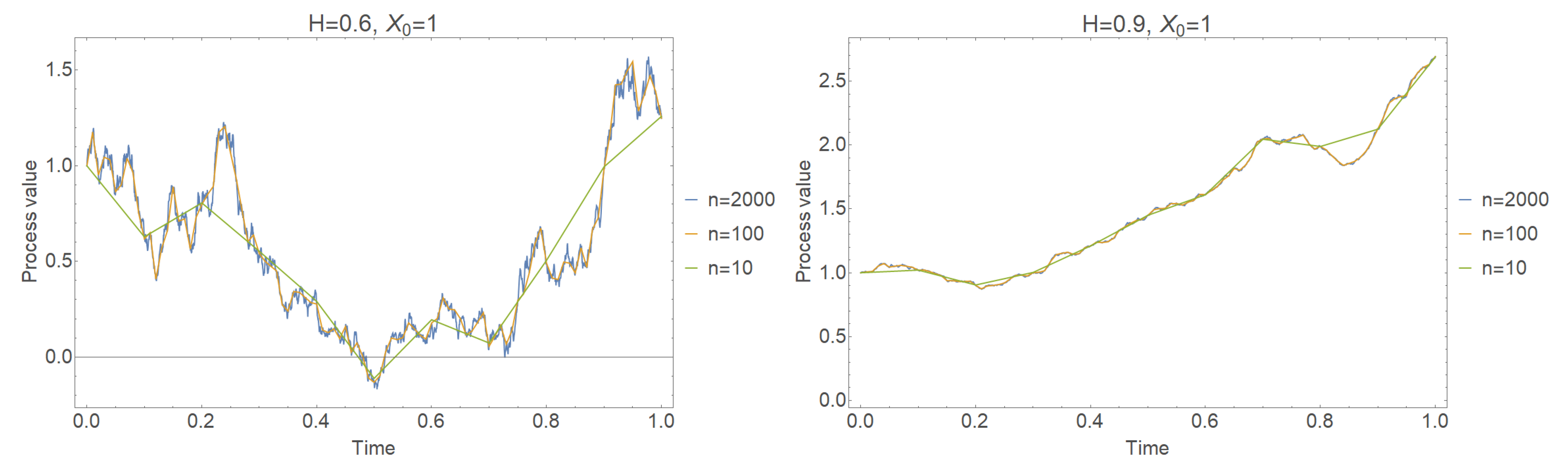
Now, using this finalized Scheme (20) we can generate trajectories of any process satisfying conditions of Theorem 1 (see Figure 1).

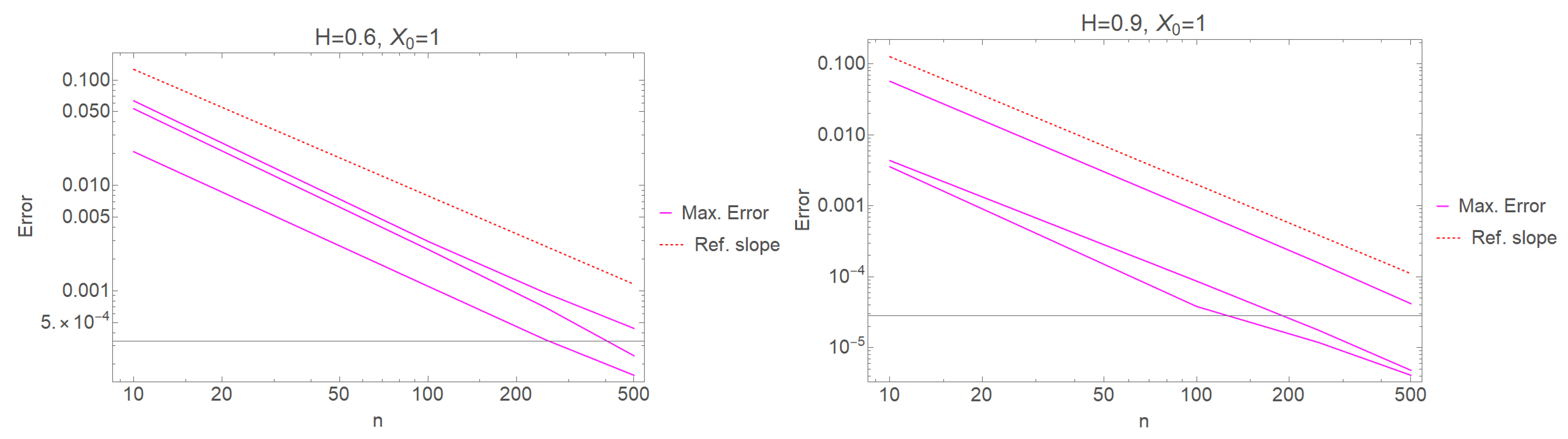
To compare the theoretical and empirical convergence rates of the Pearson process (19), we simulate the “exact” solution trajectories by using an approximation scheme (20) for a comparatively much smaller step size $h=2\times {10}^{-3}$. Since the object of the numerical experiment is investigation of the convergence rate, which is not dependent on the values of constants, the most basic set of values for (16) is sufficient (i.e., $X_0=a={\sigma }_2=1,b={\sigma }_0={\sigma }_1=2$). We see from Figure 2 that the empirical maximum error coincides with the theoretical result in Theorem 2 (reference slope).

Of course, it should be noted that we assume fBm values $B_t^H$ provided by Wolfram Mathematica programming language function FractionalBrownianMotionProcess to be not approximate but "true" values of fractional Brownian motion and that the same assumption is being made about the approximation of integrated fBm too.

5. Conclusions

We introduced an improved type of approximation scheme for certain SDEs. In comparison with the previous research in the field, due to less strict conditions, this approximation covers a wider class of stochastic processes and is proven to have a higher convergence rate. These theoretical results were supported by numerical experiments. Furthermore, we proposed a simple and direct approximation scheme with estimated convergence rate for integrated fractional Brownian motion, which can be applied by other authors modelling their own approximation schemes.

References

- Nualart, D.; Răşcanu, A. Differential equations driven by fractional Brownian motion. Collect. Math. 2002, 53, 55–81. [Google Scholar]
- Hu, Y.; Nualart, D.; Song, X. A singular stochastic differential equation driven by fractional Brownian motion. Stat. Probab. Lett. 2008, 78, 2075–2085. [Google Scholar] [CrossRef] [Green Version]
- Mishura, Y.; Yurchenko-Tytarenko, A. Fractional Cox–Ingersoll–Ross process with non-zero “mean”. Mod. Stoch. Theory Appl. 2018, 5, 99–111. [Google Scholar] [CrossRef]
- Zhang, S.Q.; Yuan, C. Stochastic differential equations driven by fractional Brownian motion with locally Lipschitz drift and their Euler approximation. Proc. R. Soc. Edinb. A 2021, 151, 1278–1304. [Google Scholar] [CrossRef]
- Kubilius, K. Estimation of the Hurst index of the solutions of fractional SDE with locally Lipschitz drift. Nonlinear Anal. Model. Control 2020, 25, 1059–1078. [Google Scholar] [CrossRef]
- Kubilius, K.; Medžiūnas, A. Positive solutions of the fractional SDEs with non-Lipschitz diffusion coefficient. Mathematics 2021, 9, 18. [Google Scholar] [CrossRef]
- Mishura, Y.; Shevchenko, G. Mixed stochastic differential equations with long-range dependence: Existence, uniqueness and convergence of solutions. Comput. Math. 2012, 64, 3217–3227. [Google Scholar] [CrossRef] [Green Version]
- Kloeden, P.; Neuenkirch, A. The pathwise convergence of approximation schemes for stochastic differential equations. LMS J. Comput. Math. 2007, 10, 235–253. [Google Scholar] [CrossRef] [Green Version]
- Kloeden, P.E.; Neuenkirch, A. Recent Developments in Computational Finance Foundations, Algorithms and Applications; World Scientific: Singapore, 2013. [Google Scholar]
- Deya, A.; Neuenkirch, A.; Tindel, S.A. Milstein-type scheme without Lévy area terms for SDEs driven by fractional brownian motion. Ann. L’I.H.P. Probab. Stat. 2012, 48, 518–550. [Google Scholar] [CrossRef]
- Jamshidi, N.; Kamrani, M. Convergence of a numerical scheme associated to stochastic differential equations with fractional Brownian motion. Appl. Numer. Math. 2021, 167, 108–118. [Google Scholar] [CrossRef]
- Neuenkirch, A.; Nourdin, I. Exact rate of convergence of some approximation schemes associated to SDEs driven by a fractional Brownian motion. J. Theoret. Probab. 2007, 20, 871–899. [Google Scholar] [CrossRef] [Green Version]
- Neuenkirch, A. Optimal pointwise approximation of stochastic differential equations driven by fractional Brownian motion. Stoch. Process Their Appl. 2008, 118, 2294–2333. [Google Scholar] [CrossRef] [Green Version]
- Mishura, Y.; Shevchenko, G. The rate of convergence for Euler approximations of solutions of stochastic differential equations driven by fractional Brownian motion. Int. J. Probab. Stoch. Process. 2008, 80, 489–511. [Google Scholar] [CrossRef] [Green Version]
- Alfonsi, A. Strong order one convergence of a drift implicit Euler scheme: Application to the CIR process. Stat. Probab. Lett. 2013, 83, 602–607. [Google Scholar] [CrossRef] [Green Version]
- Dereich, S.; Neuenkirch, A.; Szpruch, L. An Euler-type method for the strong approximation of the Cox–Ingersoll–Ross process. Proc. R. Soc. A Math. Phys. Eng. Sci. 2012, 468, 1105–1115. [Google Scholar] [CrossRef] [Green Version]
- Neuenkirch, A.; Szpruch, L. First order strong approximations of scalar SDEs defined in a domain. Numer. Math. 2014, 128, 103–136. [Google Scholar] [CrossRef]
- Hong, J.; Huang, C.; Kamrani, M.; Wang, X. Optimal strong convergence rate of a backward Euler type scheme for the Cox–Ingersoll–Ross model driven by fractional Brownian motion. Stoch. Process Their Appl. 2020, 130, 2675–2692. [Google Scholar] [CrossRef] [Green Version]
- Medžiūnas, A. On the Congruence of Finite Generalized Harmonic Numbers Sums Modulo p2. Ann. Pol. Math 2020, 126, 279–292. [Google Scholar] [CrossRef]
- Abundo, M.; Pirozzi, E. On the Integral of the Fractional Brownian Motion and Some Pseudo-Fractional Gaussian Processes. Mathematics 2019, 7, 991. [Google Scholar] [CrossRef] [Green Version]
- Kubilius, K.; Mishura, Y.; Ralchenko, K. Parameter Estimation in Fractional Diffusion Models; Bocconi & Springer Series; Springer: Berlin/Heidelberg, Germany, 2017. [Google Scholar]
Figure 1.
Approximation trajectories of Pearson process for conditions (19).
Figure 2.
Maximum error of several approximation trajectories of Pearson process for conditions (19) in comparison to reference slope.
Publisher’s Note: MDPI stays neutral with regard to jurisdictional claims in published maps and institutional affiliations. |
© 2022 by the authors. Licensee MDPI, Basel, Switzerland. This article is an open access article distributed under the terms and conditions of the Creative Commons Attribution (CC BY) license (https://creativecommons.org/licenses/by/4.0/).
Share and Cite
MDPI and ACS Style
Kubilius, K.; Medžiūnas, A. Pathwise Convergent Approximation for the Fractional SDEs. Mathematics 2022, 10, 669. https://0-doi-org.brum.beds.ac.uk/10.3390/math10040669
AMA Style
Kubilius K, Medžiūnas A. Pathwise Convergent Approximation for the Fractional SDEs. Mathematics. 2022; 10(4):669. https://0-doi-org.brum.beds.ac.uk/10.3390/math10040669
Chicago/Turabian StyleKubilius, Kęstutis, and Aidas Medžiūnas. 2022. "Pathwise Convergent Approximation for the Fractional SDEs" Mathematics 10, no. 4: 669. https://0-doi-org.brum.beds.ac.uk/10.3390/math10040669
Note that from the first issue of 2016, this journal uses article numbers instead of page numbers. See further details here.