Infrared Small Target Detection Based on Partial Sum Minimization and Total Variation

Abstract

In the advanced applications, based on infrared detection systems, the precise detection of small targets has become a tough work today. This becomes even more difficult when the background is highly dense in addition to the nature of small targets. The problem raised above is solved in various ways, including infrared patch image (IPI) based methods which are considered to have the best performance. In addition, the greater shrinkage of singular values in the methods based on IPI leads to the problem of nuclear norm minimization (NNM), which leads to the problem of incorrectly recognizing small targets in a highly complex background. Hence, this paper proposed a new method for infrared small target detection (ISTD) via total variation and partial sum minimization (TV-PSMSV). The proposed TV-PSMVS in this work basically replaces the IPI’s NNM with partial sum minimization (PSM) of singular values and, additionally, the total variance (TV) regularization term is inducted to the background patch image (BPI) to suppress the complex background and enhance the target object of interest. The mathematical solution of the proposed TV-PSMSV approach was performed using alternating direction multiplier (ADMM) to verify the proposed solution. The experimental evaluation using real and synthetic data set was performed, and the result revealed that the proposed TV-PSMSV outperformed existing referenced methods in the terms of background suppression factor (BSF) and the signal to gain ratio (SCRG).

1. Introduction

Early warning systems, video surveillance systems, military services and infrared search and track systems (IRST) are all examples of applications that use infrared small target detection (ISTD) technology. The object of interest usually remains in the complex background and is tough to detect due to the low noise ratio [1,2]. In general, ISTD approaches can be classified into two categories: sequential detection (SD) methods and single-frame detection (SFD) methods. To estimate the precise location of small targets, SD approaches such as 3-D matching filters [3,4] use both spatial and temporal information in the image. On the other hand, SFD algorithms are more reliable and efficient. TDMMS (two-dimensional least-mean squares) [5] max-mean and max-mean filters [6,7], and other SFD algorithms are the common examples. A human visual system (HVS) [8,9] based on ISTD has been recently introduced where the target is considered to be the most prominent object. Local contrast measure (LCM) [2] and its extended version are the highly researched saliency-based approaches.

Another type of technique treats the detection of small targets as a binary classification issue. Some of the well-known approaches in this class [10,11] are principal component analysis (PCA) [12] and its extended version [13]. Wang et al. [14] built a large sea-sky background dictionary to overcome the dictionary sample difficulties. Wang et al. [15] employed the parameter of study weight to bifurcate the object of interest from the background. The first work using patch image was coined by Gao et. al. and gave an IPI model to handle the problem of ISTD [1]. This IPI based model assumes that the background patch image has the non-local self-correlation characteristic. Continuing this work, Y. He et al. [16] presented a method based on sparse and low-rank representations for ISTD. Inspired by this, Zhang et al. [17] proposed a block-diagonal adaptive target-constrained representation method for sparse target separation and low-rank backgrounds.

The current IPI-based methods are affected by a difficult problem called l₁-norm sparsity issue, as a result of which these methods cannot accurately detect the background and sometimes fail to classify the target component in the target image. Dai et al. [18] has proposed a new method using the structural information of the background image, which has better performance than other methods. However, this method requires calculating the weight of the column, which is a difficult task. Dai et al. [19] again created a new non-negative IPI model that uses the partial sum of the least sum of the singular values to correctly and accurately estimate the background and preserve the large singular values.

The main drawback of this strategy is the difficulty in determining the energy constraint ratio as well as the ranking of the metrics. To overcome which Gao et al. [20] Reweighted IPI (ReWIPI) was proposed to restrict the background patch image while preserving the background edge information, which is based on the work of [21]. Similar work was proposed in [22] However, even this may result in incorrect singular value decomposition (SVD) calculations due to poor weight adjustment.

In [23], a proposal that used TV regularization and principal component pursuit (TV-PCP) to provide intrinsic smoothness to the background patch image and another method [24] based on the LP norm and TV was also proposed. Work on small target detection method based on the TV norm is mentioned in [25]. Some recent developments in IPI based approaches are also available in the literature, including reweighted IPI and tensor model with both nonlocal and local prior information [26] and non-convex rank approximation minimization [27,28]. Due to the small size of the target and the fact that the background seems to be highly diversified in character, the small target recognition task is extremely tough. However, current IPI approaches have had a lot of success in recent years. Nonetheless, our findings revealed significant flaws that may have hampered the performance of these cutting-edge approaches.

The initial flaw with these approaches was the improper estimate of background patch images (BPI) using NNM, due to l1-norm-based sparsity issues. Another difficulty was the constant weighting option, which controls the background versus target patch image trade-off. Inconsistency is caused by both the low rank qualities of the background and the sparsity property of the small target image. Such a result, having a global constant weighting parameter, as in [19], is not a smart idea. Taking these problems into account, Dai et al. [18] provided a proposal based on an adaptive column-wise weight parameter. However, the performance of this method suffers due to additional processing required for calculation of column-wise weights. As the present IPI approach uses NNM to restrict the background patch image, edges in a highly varied background might be falsely recognised as a target point owing to excessive shrinking of singular values. To solve this issue, the PSMSV has been substituted for the NNM in the current IPI model, since it preserves the important features present in the background scene. The reason for using PSMSV is that it preserves the large singular values and only minimize variance in the residual rank, which basically minimize the noise variance of observed data and not the whole data matrix. Second, the TV regularisation term was used to the IPI model’s background patch image in order to keep strong edges while enhancing the small target.

In this study, a TV-PSMSV-based approach is proposed, which combines TV regularisation with PSMSV. Further, the mathematical solution of transformation optimization using ADMM of the proposed method is presented and, finally, experimental evaluation was used for the verification of performance.

The following is a summary of the research work’s main contribution:

• An ISTD method called TV-PSMSV has been introduced in which a TV term was inducted to the BPI model to obtain more detailed features in the scene. Moreover, the PSMSV was adopted to limit BPI.
• The suggested TV-PSMSV model used an ADMM-based method to address image transformation optimization.
• The suggested model was experimentally evaluated using standard data sets; the findings revealed that it outperforms the referred state-of-the-art technique [1,18,19,20].

The remainder of the paper is laid out as follows. The technique of the suggested method is detailed in depth in Section 2. Section 3 describes the proposed method’s experimental findings using the original, noisy, and synthetic images of infrared image sequences, as well as its comparison to existing baseline approaches. In Section 4, the final conclusion is outlined.

2. Materials and Methods

This section presents the proposed TV-PSMSV method, the second part of the section outlines the TV-PSMSV model, the last subsection introduces mathematical transformation and optimization of the image using ADMM technology.

2.1. Total Variation (TV)

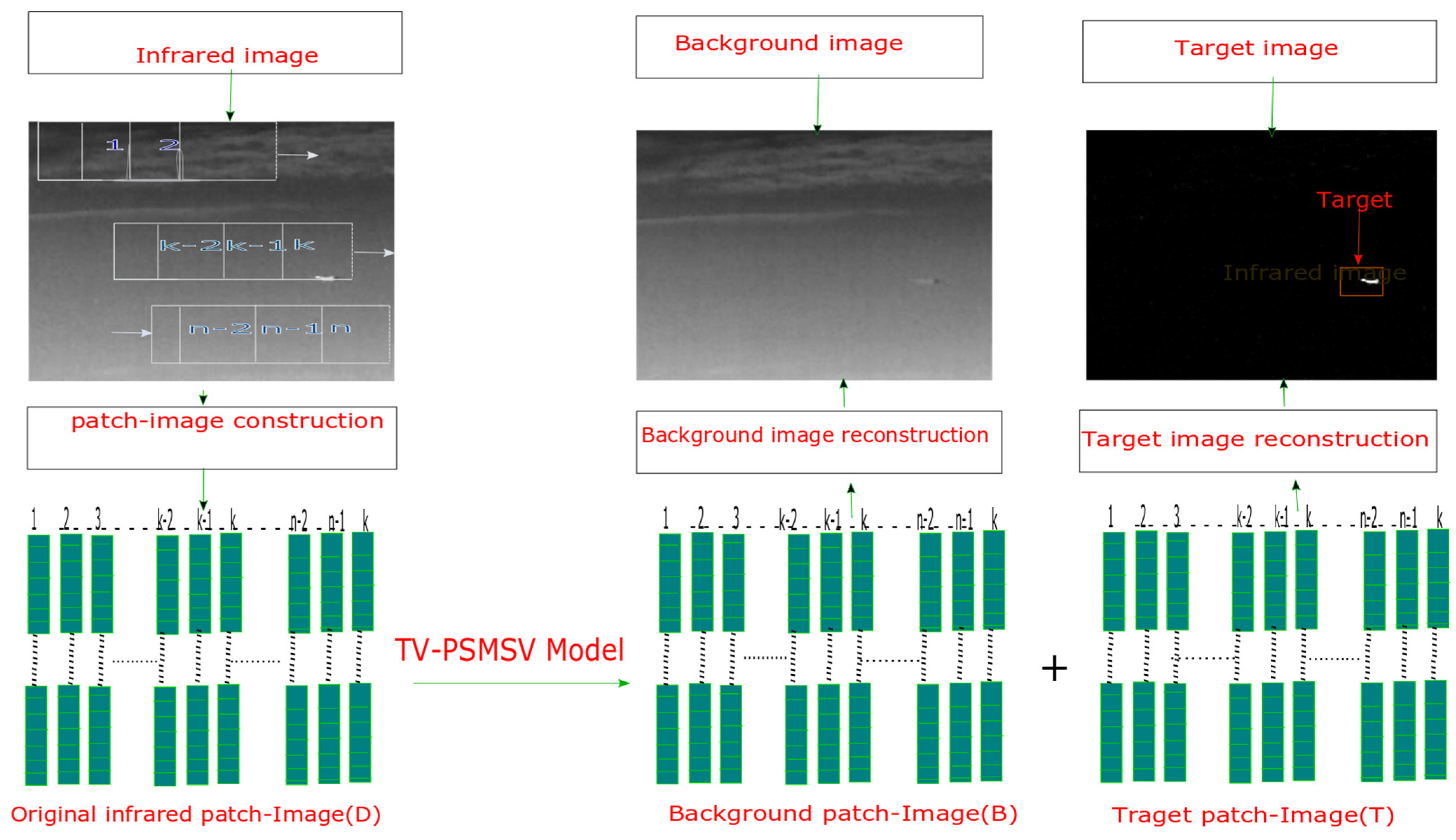
An approach based on total variation regularisation was introduced by Rudin et al. [29] is used in numerous applications of image processing. The TV model demonstrated how the TV standard may preserve the edges and corners of an image without sacrificing any details. Let $U\in R^{x\times y}$ indicate an image, and Equations (1) and (2) define the discretised anisotropic $T{V}^A$ and isotropic $T{V}^I$ of an image, respectively (2).

$$T{V}^A\left(U\right)={\displaystyle \sum }_{i=1}^x{\displaystyle \sum }_{j=1}^{y-1}\left|U_{i,j}-U_{i,j+1}\right|+{\displaystyle \sum }_{i=1}^{x-1}{\displaystyle \sum }_{j=1}^y$$

(1)

$$T{V}^I={\displaystyle \sum }_{i=1}^{x-1}{\displaystyle \sum }_{j=1}^{y-1}{\left( \begin{array}{c}{\left|U_{i,j}-U_{i,j+1}\right|}^2+\\ {\left|U_{i,j}-U_{i+1,j}\right|}^2\end{array}\right)}^{\frac{1}{2}}+{\displaystyle \sum }_{j=1}^{y-1}\left|U_{x,j}-U_{x,j+1}\right|+{\displaystyle \sum }_{i=1}^{x-1}\left|U_{i,y}-U_{i+1,y}\right|$$

(2)

Let, $D_i$U$\in R^2$ represent the discrete gradient of U at pixel I; image U is vectorized as a column vector and $D_i$ represents the gradient operator of image. Then $TV\left(U\right)$ can be finally represented as given in Equation (3):

$$TV\left(U\right)={\displaystyle \sum }_i{\Vert D_i\left(U\right)\Vert }_2.$$

(3)

2.2. TV-PSMSV Model

Single frame images are represented in the following way:

$$f_o\left(x,y\right)=f_B\left(x,y\right)+f_T\left(x,y\right)+f_N\left(x,y\right)$$

(4)

where $f_o,f_B,f_T,f_N$ are the original, background, target, noise image, and (x,y) is position of pixels in the image sequentially. Gao et al. [1], firstly, adopted (Equation (4)) in the (IPI) model-formulated target background method as below:

$$D=T+B+N,$$

(5)

where, D, B, T, and N are the input patch-image, BPI, and the target patch-image (TPI) and the noise patch-image (NPI), respectively. The low-rank BPI matrix B and the sparse TPI matrix T are decomposed from the matrix D. (Equation (5)) can be transformed into an optimization problem as stated below, and this is inspired by the method in [30].

$$\begin{gathered} \underset{B, T}{min}{\Vert B\Vert }_{*}+\lambda {\Vert T\Vert }_1, \\ s.t {\Vert D-T-B\Vert }_F\le \delta \end{gathered}$$

(6)

Here, symbol ${\Vert .\Vert }_{*}$ represents the NN of the matrix which can be calculated as the sum of singular values, symbol ${\Vert .\Vert }_1$ represents the l₁-norm and it is calculated by formula ${\Vert X\Vert }_1={\displaystyle \sum }_{ij}\left|X_{ij}\right|$, the symbol ${\Vert .\Vert }_F$ represents the Frobenius norm, which is calculated using the formula ${\Vert X\Vert }_F=\sqrt{{\displaystyle \sum }_{ij}{X}^2{}_{ij}}$, symbol $\lambda$ stands the weighting parameter and $\delta$ is the noise level of images.

2.2.1. Background Patch Image (BPI)

The BPI is derived from a combination of low-rank subspace clusters as described in [1], and NNM is used to calculate the BPI. Current target-background separation approaches, such as IPI [1], WIPI [18], and [19], use NNM to restrict the BPI. Because NNM treats all singular values the same, it shrinks them with the same threshold. As a result, instead of using NNM, the proposed method used PSMSV [31] to estimate background owing to inadequate samples. This is because PSMSV retains the larger singular values and minimises noise.

Using PSMSV, the BPI matrix B may be defined as:

$$\{\begin{array}{c}\left|{\Vert B\Vert }_{*}-{\Vert P_{N}B\Vert }_{*}\right|=\left|{\displaystyle {\displaystyle \sum }_{i=1}^{min\left(m, n\right)}}{\sigma }_{i}B-{\displaystyle {\displaystyle \sum }_{i=1}^N}{\sigma }_{i}B\right|\\ ={\displaystyle {\displaystyle \sum }_{i=N+1}^{min\left(m, n\right)}}{\sigma }_{i}B={\Vert B\Vert }_{*,\le r}\\ ={\Vert B\Vert }_{p=N}, \end{array}$$

(7)

where symbols representation as follows:

${\sigma }_{i}B$—the ith singular value of B (arranged in descending order), r—the upper limit ratio of ${\sigma }_N\left(B\right) \mathrm{and} {\sigma }_1\left(B\right) \mathrm{is} \mathrm{equal} \mathrm{to} \frac{{\sigma }_N\left(B\right)}{{\sigma }_1\left(B\right)},$ ${\Vert B\Vert }_{p=N}$—the target rank of B.

2.2.2. Target Patch-Image (TPI)

Infrared images do not have a defined size for the small target. As a result, the detection system may consider the TPI to be a sparse matrix. The l₁-norm may be used to calculate TPI in an infrared image, as demonstrated below in Equation (8).

$${\Vert T\Vert }_1=\left({{\displaystyle \sum }}_{ij}\left|T_{ij}\right|\right)$$

(8)

2.2.3. Noise Patch-Image (NPI)

It is reasonable to consider that the NPI follows the Gaussian noise distribution as described in Equation (9).

$${\Vert D-T-B\Vert }_F\le \delta$$

(9)

Here, ${\Vert .\Vert }_F$ stands for Frobenius Norm, and $\delta$ values varied depending on the image.

Finally, in addition to PSMSV, the TV regularisation term was included with the BPI. The following is the formulation of the suggested PSMSV-TV model:

$$\begin{gathered} \underset{B,T}{min}{\Vert B\Vert }_{*,\le r}+{\lambda }_{1}TV\left(B\right)+{\lambda }_2{\Vert T\Vert }_1, \\ s.t D=B+T+N, {\Vert N\Vert }_F\le \delta \end{gathered}$$

(10)

where TV$(.)$ represents the TV norm and ${\lambda }_1,{\lambda }_2$ are the constant parameter. The Equation (9) can be written as below:

$$\begin{gathered} \underset{B,T}{min}{\Vert B\Vert }_{*,\le r}+{\lambda }_2{\Vert T\Vert }_1+{\lambda }_1{\displaystyle \sum }_i{\Vert D_{i}B\Vert }_2, \\ s.t D=T+N+B, {\Vert N\Vert }_F\le \delta \end{gathered}$$

(11)

Here, $D_i$ is the gradient operator.

Finally, the proposed model applied a post-processing method on the TPI, to detect the object effectivily.

2.3. Mathematical Solution of the PSMSV-TV Model Using ADMM

We may further reformulate the aforementioned minimization issue given in Equation (11) by breaking it into sub-problems by using splitting variables as given below:

$$\begin{array}{c}\underset{Z_1,Z_2,Z_3}{min}{\Vert Z_1\Vert }_{*,\le r}+{\lambda }_2{\Vert Z_3\Vert }_1+{\lambda }_1{\displaystyle {\displaystyle \sum }_i}{\Vert z_i\Vert }_2\\ s.t Z_1=B,Z_2=\left[z_1;z_2;z_3\dots \dots ;z_{mn}\right],z_i=D_{i}B,\\ Z_3=T,D=N+T+B,{\Vert N\Vert }_F\le \delta \end{array}$$

(12)

The formulation of augmented Lagrangian function of above Equation (12) is derived in Equation (13).

$$\begin{gathered} L_A=\underset{P_1,P_2,P_3}{min}{\Vert P_1\Vert }_{*,\le r}+{\lambda }_1{{\displaystyle \sum }}_i{\Vert p_i\Vert }_2+{\lambda }_2{\Vert P_3\Vert }_1+\langle L_1,Z_{1}B\rangle +\frac{\beta }{ 2}{\Vert P_1-B\Vert }_F{}^2 \\ +{{\displaystyle \sum }}_i\langle l_{i },p_i-D_{i}B\rangle +\frac{{\beta }_i}{2}{\Vert p_i-D_{i}B\Vert }_F{}^2+\langle L_3,P_{3}T\rangle +\frac{\beta }{2}{\Vert P_3-T\Vert }_F{}^2+ \\ \langle L_4, D-N-T-B\rangle +\frac{\beta }{2}{\Vert D-N-T-B\Vert }_F{}^2 \end{gathered}$$

(13)

The standard trace inner product for the matrix of vectors is denoted by. The Lagrange multipliers are $L_1,L_2,L_3$ and $L_4$ and the penalty parameter is >0. Each variable T, B, $P_1,P_2, \mathrm{and} P_3$ in Equation (13) are vectorized to column vectors for simplicity. The optimization problem of image matrix is mathematically solved using the ADMM [30,32]; it is solved in every iteration by minimising each of the T, B, $P_1,P_2, \mathrm{and} P_3$ variables while leaving the other variables constant. Lastly, the Lagrange multipliers have been modified as follows:

$$\{\begin{array}{c}{L}_1{}^{k+1}\leftarrow L_1{}^k+\gamma \beta \left(P_1{}^{k+1}-B^{k+1}\right)\\ L_2{}^{k+1}\leftarrow L_2{}^k+\gamma \beta \left(P_2{}^{k+1}-D{B}^{k+1}\right)\\ L_3{}^{k+1}\leftarrow L_3{}^k+\gamma \beta \left(P_3{}^{k+1}-T^{k+1}\right)\\ L_4{}^{k+1} \leftarrow L_4{}^k+\gamma \beta \left(P_4{}^{k+1}-B^{k+1}-T^{k+1}-N^{k+1}\right)\end{array}$$

(14)

Here $\gamma >0$ represent step length.

The $P_1$ sub-problem can be represented using given below Equation (15)

$$\begin{gathered} P_1{}^{k+1}\underset{Z_1}{arg min} L_A(P_1,P_2{}^k,P_3{}^k,B^k,T^k) \\ \underset{Z_1}{=arg min {\Vert Z_1\Vert }_{*,\le r}}+\langle L_1,P_1-B\rangle +\frac{\beta }{2}{\Vert P_1-B\Vert }_F{}^2 \\ \underset{Z_1}{=arg min}{\Vert P_1\Vert }_{*,\le r}+\frac{\beta }{2}{\Vert P_1-\left(B^k- \frac{L_1{}^k}{\beta }\right)\Vert }_F{}^2 \end{gathered}$$

(15)

This sub-problem can be solved by applying the Theorem 1 as given below:

Theorem 1. 

Let us consider$X,L \in R^{m\times n}, \tau >0, \mathrm{and} l=min\left(m,n\right),$which can be decomposed by SVD. L can be considered as two matrices, L =$L_1+L_2$=$U_{L_1}{D}_{L_1}{V}_{l_1}{}^T$+$U_{L_2}{D}_{l_2}{V}_{L_2}{}^T$; here, $U_{L_1},V_{L_1}$are singular value matrices corresponding to N highest singular values by SVD, and$U_{L_2},V_{L_2}$from${\left(N+1\right)}^{th}$to the last singular values. Finally, the PSVM problem for singular values may be described as shown in Equation (16):

$$\underset{X}{arg min\frac{1}{2}}{\Vert X-L\Vert }_F{}^2+\tau {\Vert X\Vert }_{p=N}$$

(16)

The partial singular value thresholding operator may be used to describe the optimal solution of Equation (15), which is defined as:

$$\begin{gathered} P_{N,\tau }\left[Y\right]=U_Y\left(D_{Y_1}+S_{ \tau }\left[D_{Y_2}\right]V_Y{}^T\right) \\ =Y_1+U_{Y_2}{S}_{ \tau }\left[D_{Y_2}\right]V_{Y_2}{}^T. \end{gathered}$$

(17)

Here

$$\begin{gathered} D_{Y1} \mathrm{is} \mathrm{equal} \mathrm{to} \mathrm{diag}\left({\sigma }_{1,}\dots .,{\sigma }_{N,}0,\dots ,0\right), \\ {D}_{Y2} \mathrm{is} \mathrm{equal} \mathrm{to} \mathrm{diag}\left(0,\dots ,0,{\sigma }_{N+1,}\dots .,{\sigma }_{l,}\right) \end{gathered}$$

(18)

In addition, $S_{ \tau }\left[x\right]$ = sign$\left(x\right)$.max$\left(\left|x\right|-\tau ,0\right)$ is the thresholding operator [33,34,35]. It may be phrased as follows for the P₂ sub-problem:

$$\{\begin{array}{c}{P}_2{}^{k+1}\leftarrow \underset{Z_2}{arg min} L_A\left(P_1{}^k,P_2,P_3{}^k,B^k,T^k\right)\\ =\underset{P_2}{arg min}{\displaystyle {\displaystyle \sum }_i}\left(\begin{array}{c}{\Vert p_i\Vert }_2+\langle l_{i }{}^K,z_i-D_i{B}^K\rangle \\ +\frac{{\beta }_i}{2}{\Vert p_i-D_i{B}^K\Vert }_F{}^2\end{array}\right)\end{array}$$

(19)

Because it is a l₂ optimization problem, the sub-problem (19) may be mathematically solved using a 2-D shrinkage-like formula [36].

$$\{\begin{array}{c}{p}_i=max\left\{{\Vert D_{i}B-\frac{l_{i }}{{\beta }_i}\Vert }_2-\frac{1}{{\beta }_i},0\right\}.\frac{\left(D_{i}B-\frac{l_{i }}{{\beta }_i}\right)}{{\Vert D_{i}B-\frac{l_{i }}{{\beta }_i}\Vert }_2},\end{array}$$

(20)

The reformulation for the P₃ sub-problem can be solved using the Equation (21):

$$\{\begin{array}{c}{P}_3{}^{k+1}\leftarrow \underset{P_3}{arg min{L}_A\left(P_1{}^k,P_2{}^k,{ P}_3,P_{2 }{}^k,B^k,T^k\right)}\\ =arg min{\lambda }_2{\Vert P_3\Vert }_1,+\langle L_3,P_3-T\rangle +\frac{\beta }{2}{\Vert P_3-T\Vert }_F{}^2\\ =\underset{Z_3}{arg min}{\lambda }_2{\Vert P_3\Vert }_1+\frac{\beta }{2}{\Vert P_3-\left(T^k-\frac{L_3{}^k}{\beta }\right)\Vert }_F{}^2\end{array}$$

(21)

The Equation (21) can be further solved by given below Equations (22) and (23).

$$P_3{}^{k+1}=T{h}_{\frac{{\lambda }_2}{\beta }}\left(T^k-\frac{L_3{}^k}{\beta }\right)$$

(22)

$${Th}_{\epsilon }\left(W\right)=\{\begin{array}{c} w-\epsilon w>\epsilon \\ w-\epsilon w<-\epsilon \\ 0 otherwise \end{array}$$

(23)

where ${Th}_{\epsilon }(.)$ represent the thresholding.

For N sub-problem, the solutions may be represented as given in Equation (24)

$$\{\begin{array}{c}{N}^{k+1}\underset{N}{\leftarrow arg min}\begin{array}{c}\langle L^k{}_4, D-B^k-T^k-\end{array}N\rangle \\ +\frac{\beta }{2}{\Vert D-B-T^k-N\Vert }_F{}^2\\ ={\Vert N-\left(D-T^k-B^k+\frac{L_4{}^k}{\beta }\right)\Vert }_F{}^2\\ s.t. {\Vert N\Vert }_F\le \delta \end{array}$$

(24)

The Equation (24) can be further solved by given below Equation (25).

$$N^{k+1}=P_{\Omega }\left(D-T^k-B^k+\frac{L_4{}^k}{\beta }\right)$$

(25)

where $\Omega$ denotes the sphere of the ${\Vert .\Vert }_F\le \delta$, and the $P_{\Omega }$ is the projection onto the matching sphere.

For the B sub-problem, the solutions may be represented as given in Equation (26)

$$B^{k+1}\leftarrow \frac{\partial L_A}{\partial B}=0$$

(26)

Equation (26), for example, may be rewritten as:

$$-\frac{\partial L_A}{\partial B}=L_1{}^k+ \beta \left(P_1{}^{k+1}-B\right)+{\displaystyle \sum }_i\left[D_i{}^T{l}_{i }+{ \beta }_i{D}_i{}^T\left(p_i-D_{i}B\right)\right]+L_4{}^k+ \beta \left(D-T^{k+1}\right)$$

(27)

$$\begin{gathered} B^{k+1}={\left({\displaystyle \sum }_i\beta D_i{}^T{D}_i+2\beta \right)}^{-1} \\ \left[\begin{array}{c}{L}_1{}^k+L_4{}^k+\left({\displaystyle {\displaystyle \sum }_i}\left[{\beta }_i{D}_i{}^T\left(p_i-D_{i}B\right)+D_i{}^T{l}_{i }\right]\right)\\ +\beta \left(P_1{}^{k+1}-T+D\right)\end{array}\right] \end{gathered}$$

(28)

Sub-problem may be handled in the same way as B sub-problem:

$$T^{k+1}\leftarrow \frac{\partial L_A}{\partial T}=0$$

(29)

$$T^{k+1}=\frac{L^k+ \beta \left(D-B^{k+1}\right)+\beta p_3{}^{k+1}+L_4{}^k}{2\beta }$$

(30)

2.4. Modelling for Small Target Extraction from Background Image

The entire target-background extraction process using the PSMSV-TV paradigm is depicted by Figure 1 and is described as given below steps:

A: 

Creation of patch image from Input:

This is the initial phase, when an infrared patch image called D was created using the original image $f_D$ from the image sequence. A sliding window moved from left to right first and then moved down from top to bottom to create the patch-images.

B: 

Target background separation:

In the second phase, the input patch image was processed using Algorithm 1 to fragment it into two matrices; the first one was a B and the second was a T.

C: 

Regeneration of the target and background image:

In the third phase, the proposed method reconstructed the $f_T$, and the $f_B$ from the target patch images and the background. The whole process could be accomplished using the technique outlined in [1].

D: 

Segmentation process:

Now the final touch was initiated, where some final-processing to enhance the quality of target image was performed for the adaptive thresholding scheme was run as described in [1] and it was calculated using given Equation (31):

$$t_{up}= max\left(v_{min},\overline{f_T}+k\sigma \right)$$

(31)

Here $\sigma , \overline{f_T}$ is the standard deviation and the average of the k and $f_T$ respectively, and $v_{min}$ is taken as an empirical constant value.

Algorithm 1: The PSMSV-TV Method.

Input: Input is the original IPI $\mathit{D}$,$\beta ,\gamma ,{\lambda }_1,{\lambda }_{2,}\mathit{r}\mathit{a}\mathit{t}\mathit{i}\mathit{o} \mathit{r},$tol Output: ${\mathit{T}}^{\mathit{k}},{\mathit{B}}^{\mathit{k}}$ 1:  $\mathbf{Initialize}\mathbf{:} {\mathit{B}}^{\mathit{k}} = \mathit{z}\mathit{e}\mathit{r}\mathit{o}\mathit{s}\left(\mathit{m},\mathit{n}\right), {\mathit{T}}^{\mathit{k}} = \mathit{z}\mathit{e}\mathit{r}\mathit{o}\mathit{s}\left(\mathit{m},\mathit{n}\right), {\mathit{P}}_{\mathbf{1}} = {\mathit{P}}_{\mathbf{3}} = \mathit{z}\mathit{e}\mathit{r}\mathit{o}\mathit{s}\left(\mathit{m},\mathit{n}\right), {\mathit{L}}_{\mathbf{1}}={\mathit{L}}_{\mathbf{3}} = \mathit{z}\mathit{e}\mathit{r}\mathit{o}\mathit{s}\left(\mathit{m},\mathit{n}\right),$ ${\mathit{L}}_{\mathbf{2}} = \mathit{z}\mathit{e}\mathit{r}\mathit{o}\mathit{s} (\mathbf{2}, \mathit{mn}), {\mathit{P}}_{\mathbf{2}} = \mathit{z}\mathit{e}\mathit{r}\mathit{o}\mathit{s} (\mathit{mn}, \mathbf{2}),\mathbf{\gamma }=\mathbf{1.5},\mathit{t}\mathit{o}\mathit{l}={\mathbf{10}}^{-\mathbf{5}},$ 2:  while (not converged) do: 3:  ${\mathit{P}}_{\mathbf{1}}{}^{\mathit{k}\mathbf{+}\mathbf{1}}\mathbf{=}{\mathit{P}}_{\mathit{N},{\mathit{\beta }}^{\mathbf{-}\mathbf{1}}}\left(B^k-\frac{{\mathit{L}}_{\mathbf{1}}{}^k}{\beta }\right)$ 4:  ${\mathit{P}}_{\mathbf{2}}{}^{\mathit{k}\mathbf{+}\mathbf{1}}$ is calculated using Equation (19) 5:  ${\mathit{P}}_{\mathbf{3}}{}^{\mathit{k}\mathbf{+}\mathbf{1}}=\mathit{T}{\mathit{h}}_{\frac{{\lambda }_{\mathbf{2}}}{\beta }}\left(T^{\mathit{k}}-\frac{{\mathit{L}}_{\mathbf{3}}{}^{\mathit{k}}}{\beta }\right)$ 6:  $B^{\mathit{k}+\mathbf{1}}$ is solved by Equation (28) 7:  $T^{\mathit{k}+\mathbf{1}}$ is solved by Equation (30) 8:  ${\mathit{N}}^{\mathit{k}+\mathbf{1}}=P_{\Omega }\left(D-T^{\mathit{k}}-B^{\mathit{k}}+\frac{{\mathit{L}}_{\mathbf{4}}{}^k}{\beta }\right)$ 9:  Update ${\mathit{L}}_{\mathit{i}}\left(\mathit{i}=\mathbf{1},\mathbf{2},\mathbf{3},\mathbf{4}\right)$ according to Equation (14) 10:  Convergence checking $\frac{\Vert D-T^k-B^k{{\Vert }^2}_F}{{\Vert D\Vert }_F}<\mathit{t}\mathit{o}\mathit{l}$ 11:  k++ 12:  end while.

3. Experimental Result Analysis

In the experimental analysis, the performance of the proposed TV-PSMSV was evaluated against the referenced existing methods. This involved standard dataset preparation and comprehensive experimentation on real, noisy, and synthetic image sequences in a variety of background environments.

3.1. Dataset Preparation

The dataset for experimental evaluation consisted of 1080 infrared images with various backgrounds such as sea, sky, cloud, and ground; dataset description was presented in

Table 1. Summery of taken dataset.

Infrared Real Sequences #	Image Size	No of Frames	Target Characteristics	Target Type	Background Characteristics
# 1	256 × 200	30	The target is small in size, yet it has a great imaging range.	A small ship	Blurred sea-sky backgrounds.
# 2	256 × 200	250	The target is small in size, yet it has a great imaging range.	An airplane	High dense clouds with less local contrast
# 3	256 × 200	250	The target is small in size, yet it has a great imaging range and SRC value is low.	An airplane	With varying background
# 4	128 × 128	100	The target is small in size, yet it has a great imaging range and SRC value is low	A Helicopter	Changing background
# 5	128 × 128	200	Small size with 1 or 2 target	A ship	Changing background
# 6	280 × 228	250	The target is small in size, yet it has a great imaging range and SRC value is low	A man walking through the forest	Background with heavy clouds.

. We began by experimenting with single item infrared pictures. Second, the suppression capacity of the proposed technique was proven using picture sequences with Gaussian noise. We employed synthetic image sequences to assess the robustness of the proposed technique. In addition, we addressed how characteristics such as image patch size and sliding step size affected the outcomes. The proposed strategy has been compared with eight baseline approaches: max-mean filter [6], max-median filter [6], top-hat filter [37], IPI [1], RPCA [18], NIPPS [19], RIPT [26] and TV-PCP [23] on six distinct original infrared images. The parameter settings for all of the baseline techniques are listed in

Table 2. Summery of parameter settings for evaluation.

No.	Methods	Parameter Values
1	Max-Mean Filter [5]	Filter size 5 × 5
2	Max-Median Filter [5]	Filter size 5 × 5
3	Top-Hat filter [37]	Structure shape is 3 × 3
4	NIPPS [19]	$\mathrm{Patch} \mathrm{size}=50 \times 50, \mathrm{sliding} \mathrm{step}=10, \rho =1.5, \lambda =\frac{L}{\sqrt{min\left(m,n\right)}}, r={10}^{-3},$$L=2, \mathrm{tolerance} \mathrm{error}, \epsilon ={10}^{-7},$
5	RPCA [18]	$\mathrm{sliding} \mathrm{step}=10, \mathrm{Patch} \mathrm{size}=50 \times 50, \mathrm{tolerance} \mathrm{error} \epsilon ={10}^{-7}$$, \lambda =\frac{1}{\sqrt{m}}$
6	IPI model [1]	$\mathrm{sliding} \mathrm{step}=10, \mathrm{Patch} \mathrm{size}=50 \times 50, \mathrm{tolerance} \mathrm{error} \epsilon ={10}^{-7}$$, \lambda =\frac{1}{\sqrt{m}},$
7	RIPT [26]	$\mathrm{Patch} \mathrm{size} \mathrm{is} 50 \times 50, \mathrm{sliding} \mathrm{step} \mathrm{is} 10, \lambda =\frac{L}{\sqrt{min\left(m,n\right)}}$$,L=1,h=1, \epsilon ={10}^{-7}$
8	TV-PCP [23]	Patch size is 50 × 50, sliding step is 14, lambda = 0.005, maxIter = 250, $Tol=5 \times {10}^6, \mathrm{beta}=0.025, \mathrm{gama}=1.5, \mathrm{lambda} 2=1/\left(\mathrm{sqrt}\right(min(mm,nn)), \rho$ = 1.5
9	ISTD based on TV-PSMSV	$\mathrm{sliding} \mathrm{step}=14, \mathrm{Patch} \mathrm{size}=50 \times 50, \beta =0.025,{\lambda }_1=0.005,{\lambda }_2=\frac{L}{\sqrt{min\left(m,n\right)}},$$r={10}^{-3}, L=2, \gamma =1.5,$$\mathrm{tolerance} \mathrm{error} \epsilon ={10}^{-5}$

. The ADMM was used here to solve the procedure. All of the algorithms were implemented in MATLAB 2015a on a PC with a configuration of 2.2 GHz processor, and 4GB of RAM.

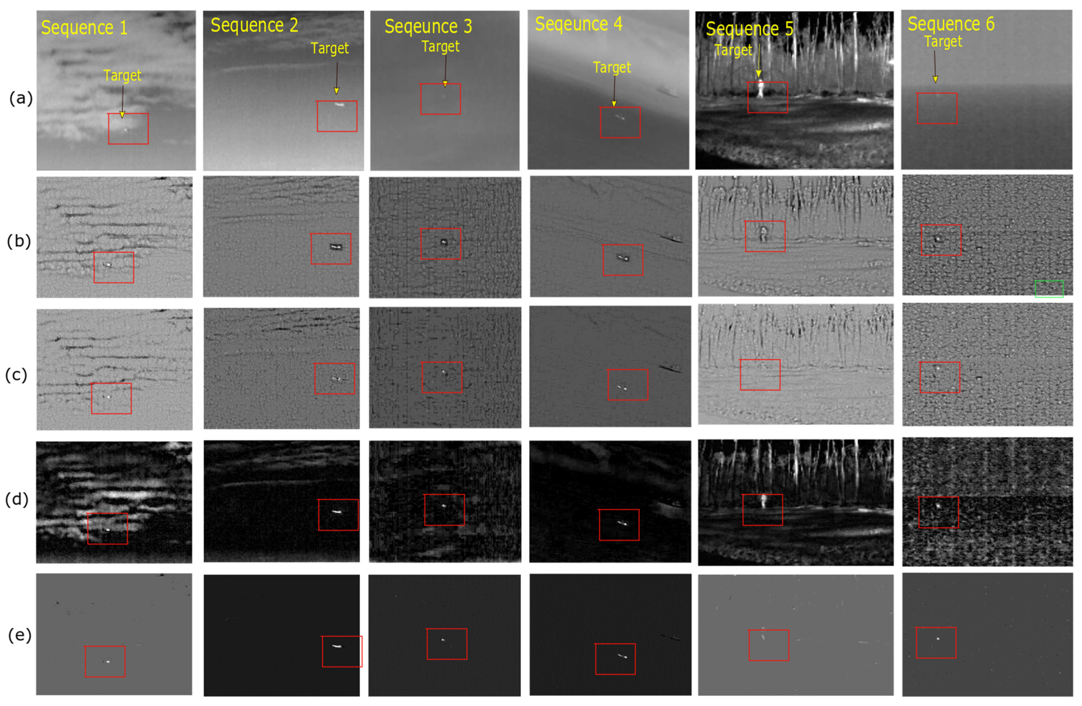
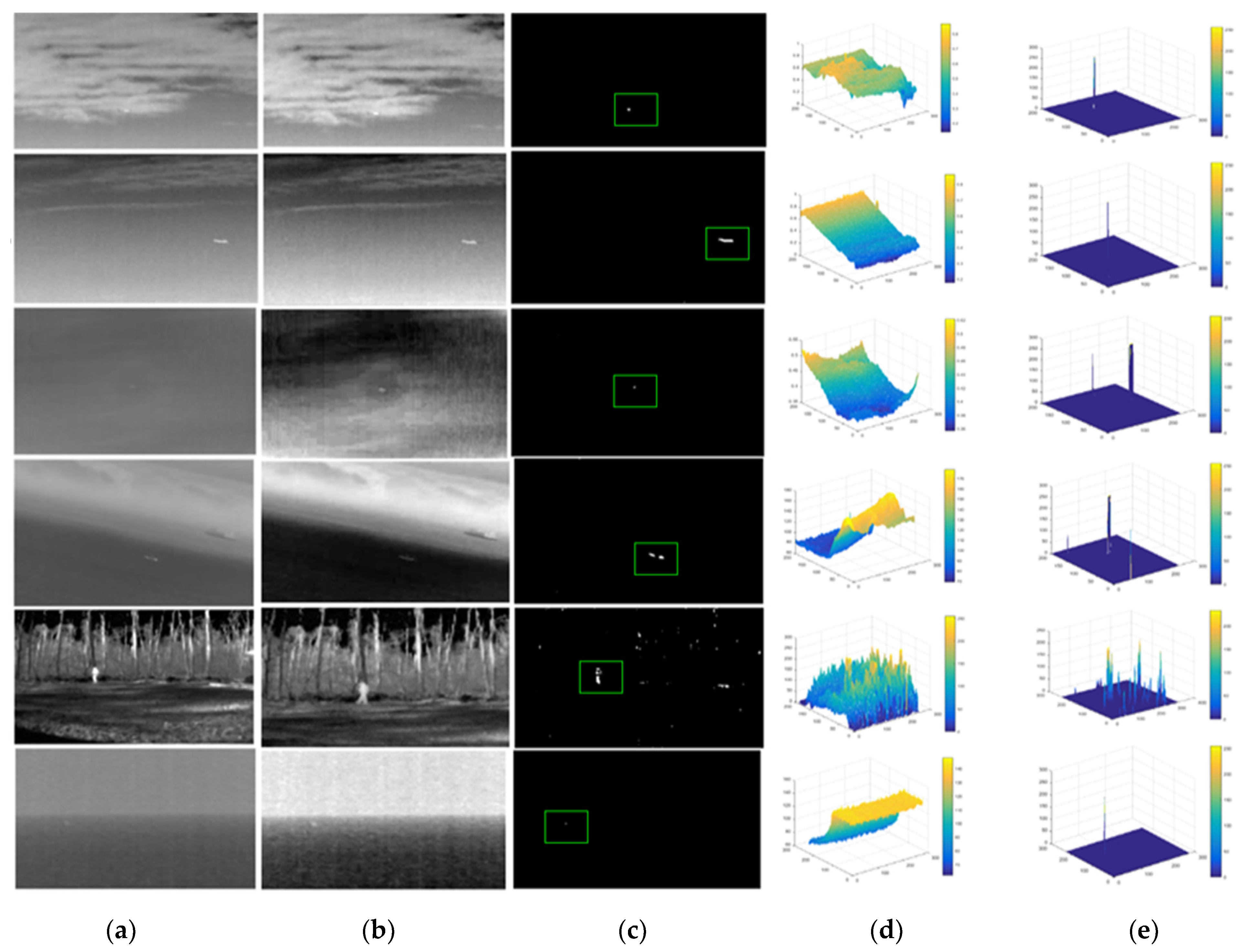
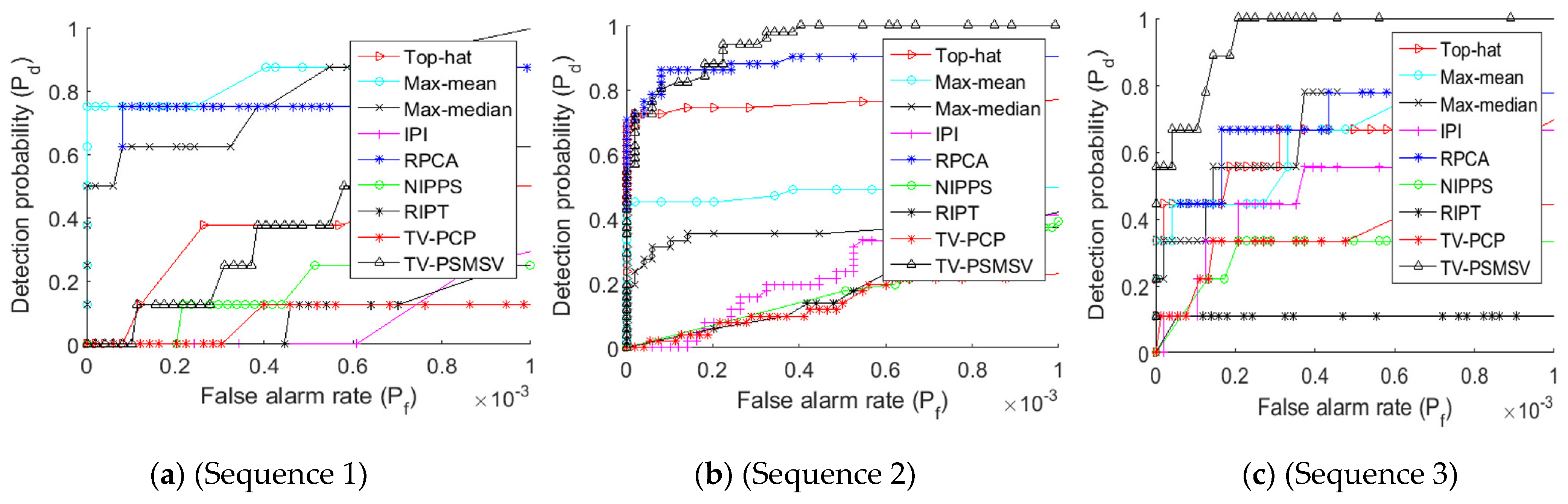
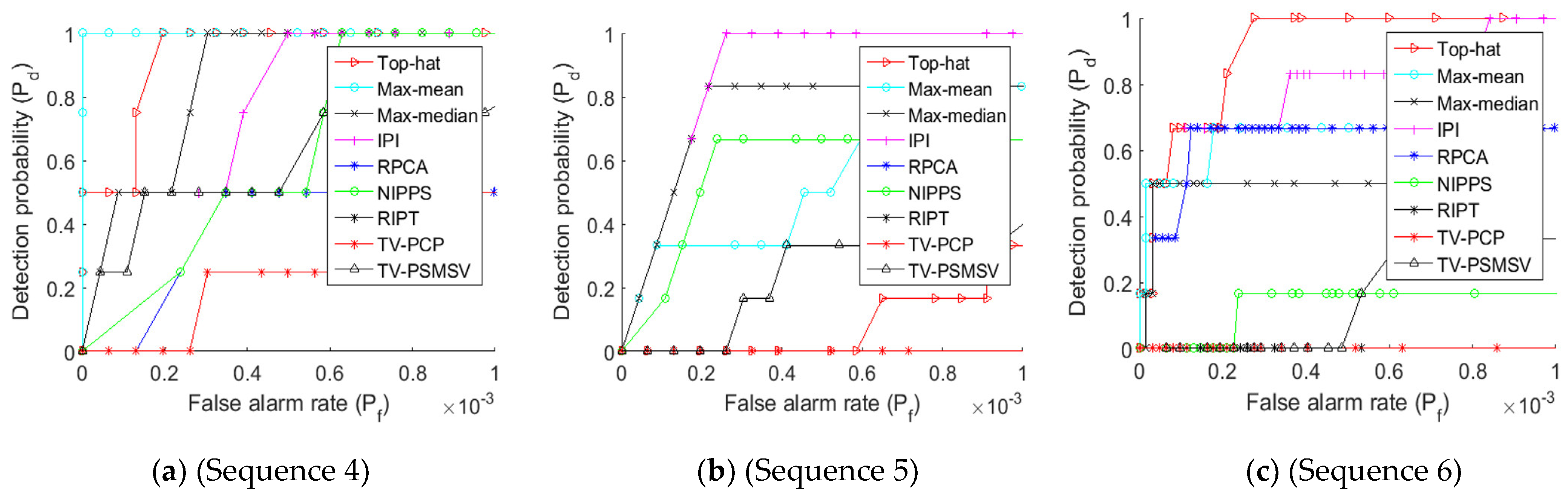
3.2. Experimental Evaluation Using Real Image Sequence

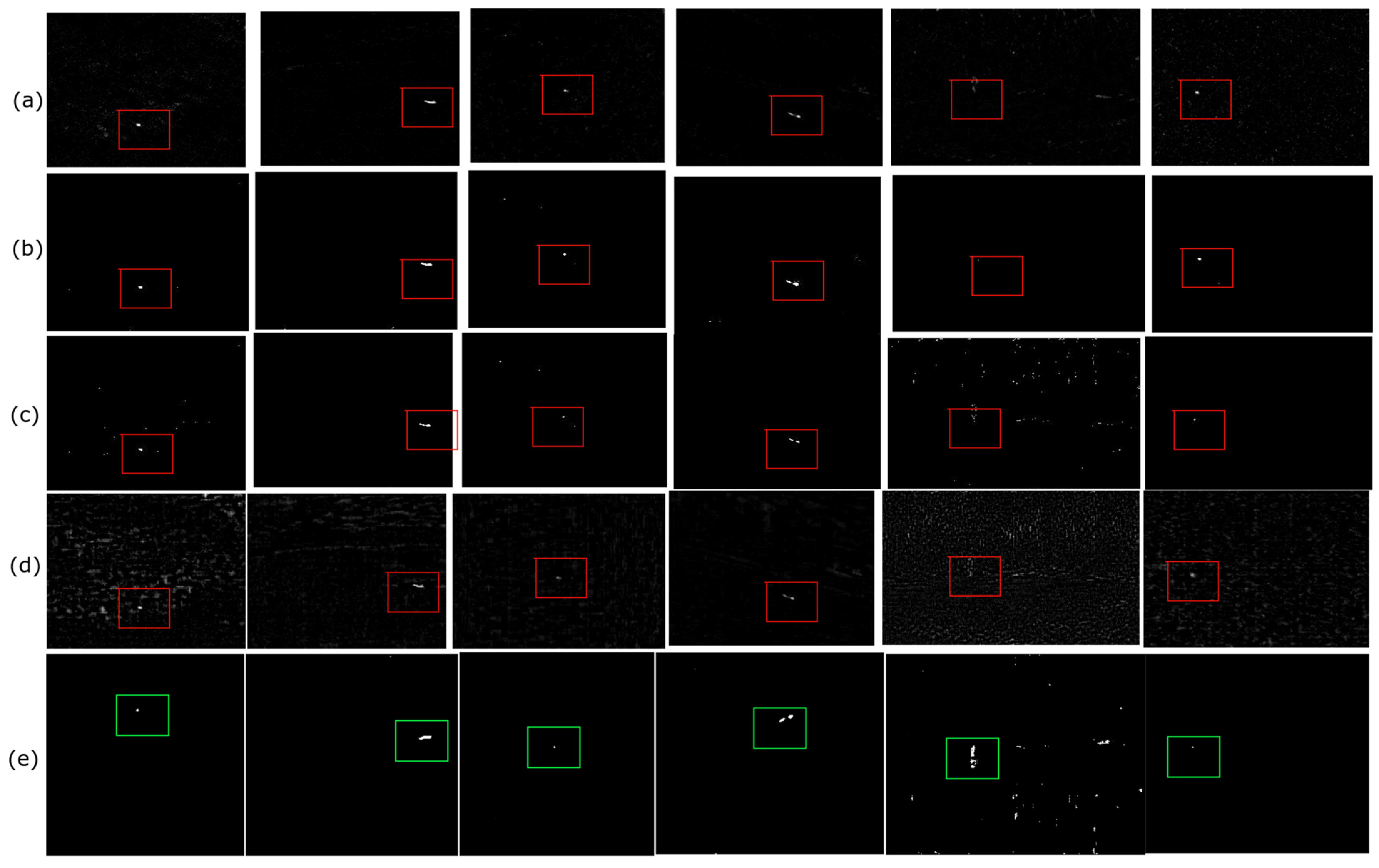
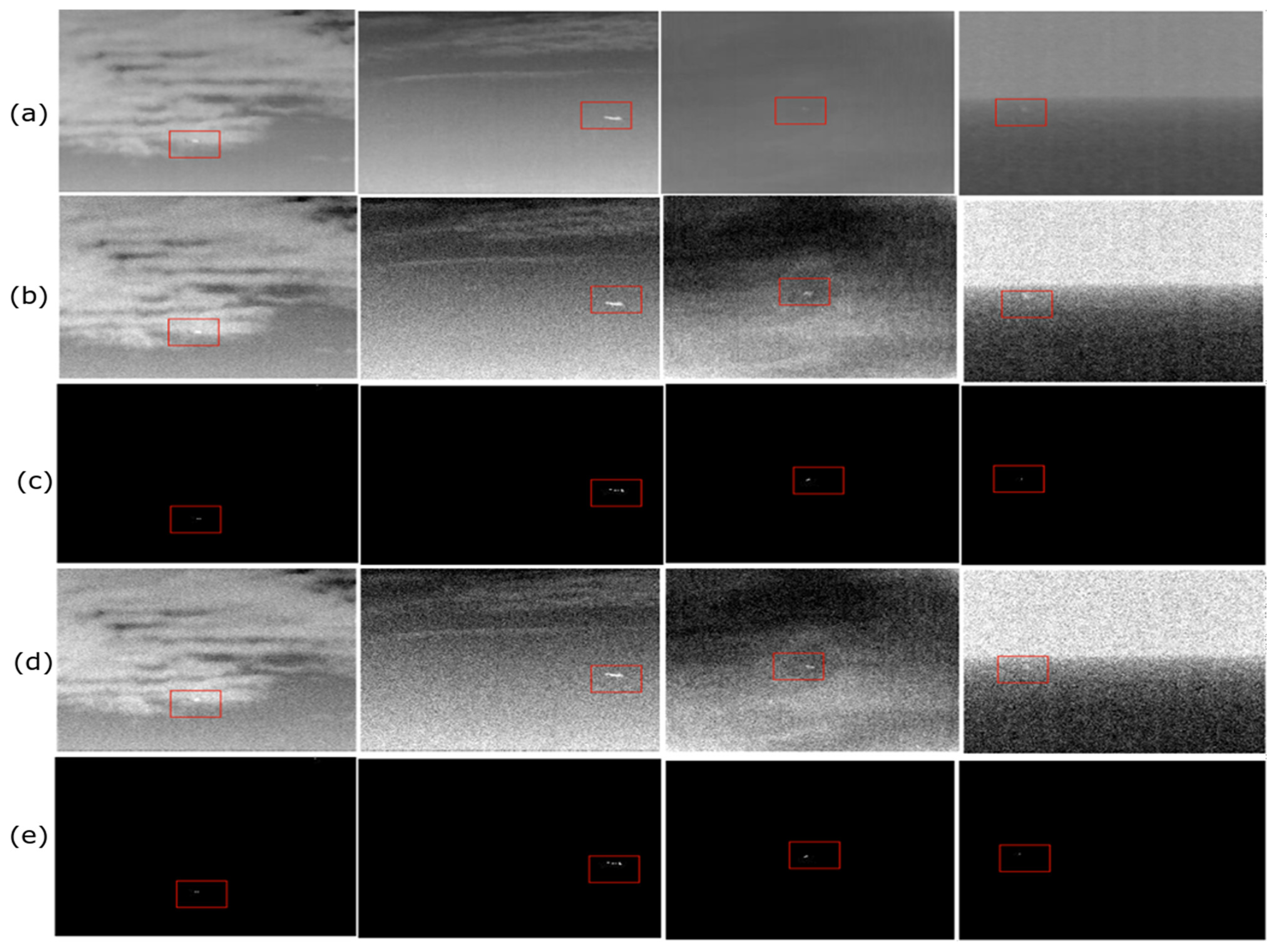
3.2.1. Evaluation of Background Suppression of Images Sequences

This section shows the experimental results of each strategy on taken dataset of six different image sequences with different complex backgrounds. In Figure 2 and Figure 3, the suggested TV-PSMSV technique is displayed alongside the max-mean filter, max-median filter [6], top-hat filter [37], IPI [1], RPCA [16], NIPPS [20], RIPT [27] and TV-PCP [23] approaches. In the Figure 2 the experimental results of Max-mean, Max-median,Top-hat and IPI methods are presented. The top hat, max-mean, and max-median methods are simple and easy to implement. Due to this reason, these methods demonstrated strong detecting skills when the background was moderately sluggish and smooth. However, they exhibited poor capability when the background was quite strong and dense.

As it can be observed from the Figure 3 that, the RPCA approach has shown good performance, but its shortcoming is that it had a fixed regulating value, making background prediction problematic at times.. The NIPPS approach utilises the partial sum minimization of singular values in place of the NNM in the IPI to contrain the background. Due to this, this method was also capable of suppressing background effectively. In addition to this, the model just minimised the noise variance without taking into account the entire data matrix, which makes this model different from the others. Although the IPI method could detect the target object quite well, this method lacked its performance due to the presence of heavy noise and l1 norm sparsity. Thus, the detection of a non-target object may be seen in the target image.

The RIPT method has impressed well in terms of target detection and background suppression ability. RIPT did not do well in the presence of noise. Although the TV-PCP method performed well, it still had issues in non-smooth background. Motivated by the work in TV-PCP [23], the inner smoothness and the sharp edges information of the background could be extracted by introducing the TV norm. Therefore, the suggested approach could smooth the background beautifully, allowing strong edges and buildings to be very easily predicted, allowing the true target to be identified smoothly. Furthermore, there may be clutter in the background of the image whose grey level was comparable to the potential target, making it harder to recognize the target object. As a result, the 3D grey map in Figure 4 could better assist in predicting the position of the small target in the image.

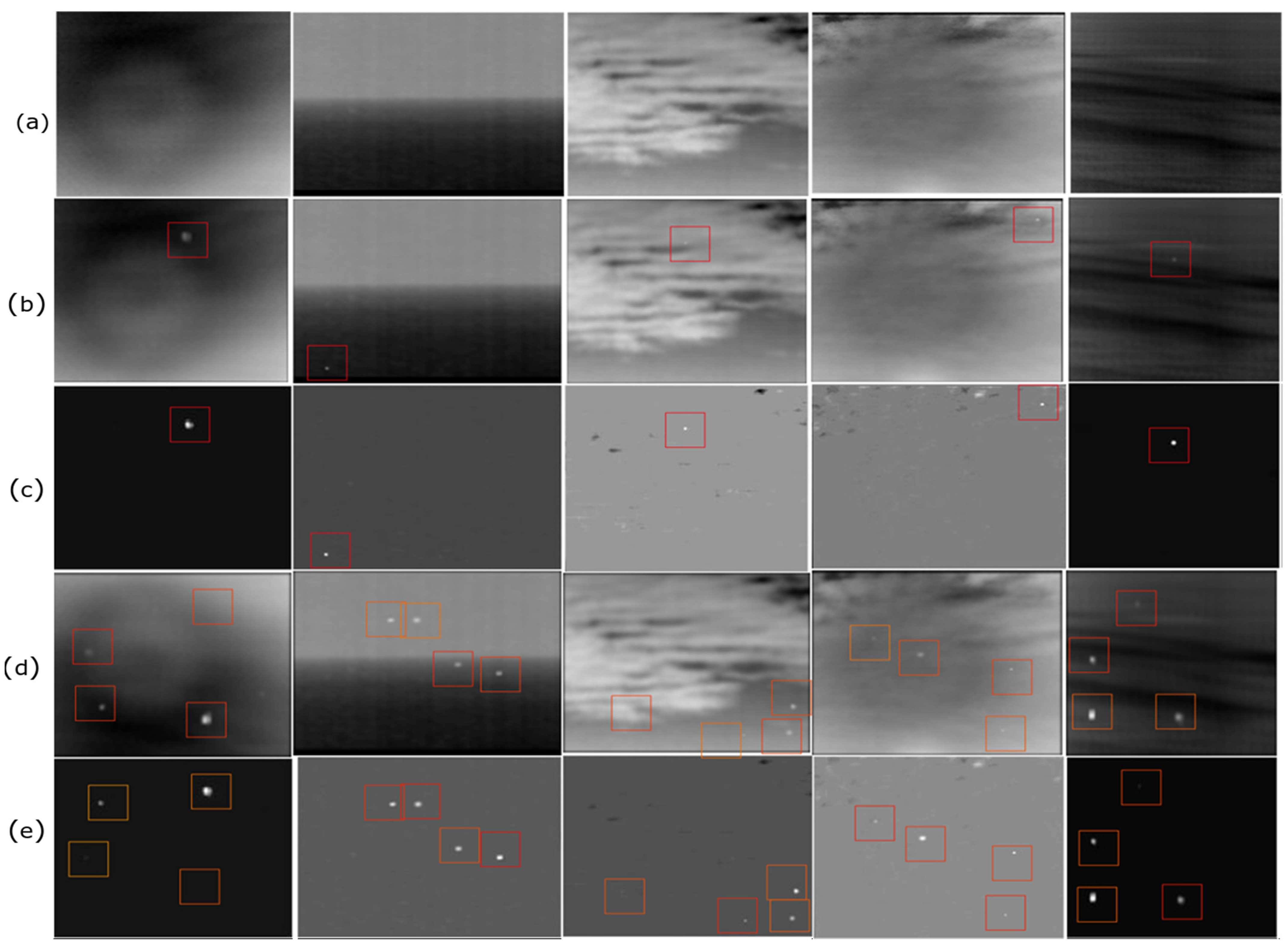
3.2.2. Evaluation of Background Suppression for Noisy Images Sequences

The next experiment was conducted in the context of noisy images. Figure 5a depicts the original image sequences, whereas Figure 5b,c depict images with Gaussian noise of 10 and 20 standard deviations (sd.), respectively. It can be seen from the findings in Figure 5d,e that the suggested technique performed better than the mentioned methods in terms of background suppression and small target detection in noisy images.

3.2.3. Experimental Evaluation on a Synthetic Image Sequences

In the third evaluation, the performance of the proposed TV-PSMSV method is validated against the synthetic image sequences. A dataset of synthetic image sequences was prepared with varied backgrounds applying real infrared images. The small targets with variable size were embedded into the background at different random locations. The synthetic dataset preparation process was clearly defined in [1]. During the experiment evaluation, one and four target image sequences were identified. In addition, the proposed TV-PSMSV’s ability to decrease background noise was evaluated; results are shown into the Figure 6.

3.3. Evaluation Metrics Indicators

In order to assess the outcome of the presented TV-PSMSV approach, two standard classical evaluation metrics were considered, namely: SCRG and background suppression factor (BSF). Detailed description of these indicators is outlined in [38] and can be represented as shown in Equation (32):

$$BSF=\frac{C_{in}}{C_{out}}, SCRG=\frac{{\left(\raisebox{1ex}{$S$}\!\left/ \!\raisebox{-1ex}{$C$}\right.\right)}_{out}}{{\left(\raisebox{1ex}{$S$}\!\left/ \!\raisebox{-1ex}{$C$}\right.\right)}_{in}}$$

(32)

Here, C and S denote the clutter standard deviation and signal amplitude, and the original input and the output target image are represented by in and out, respectively. The experimental results values of BSF and SCRG are shown in

Table 3. Observed values of BSF and SCRG.

ISTD	Evaluation Indicators	Seq1	Seq2	Seq3	Seq4	Seq5	Seq6
Top Hat	BSF	0.488	2.339	0.512	2.354	0.923	0.923
	SCRG	1.281	5.733	7.376	53.302	3.081	24.651
Max-Median	BSF	1.296	3.895	0.747	3.249	1.167	1.195
	SCRG	1.608	1.708	5.415	36.456	2.117	17.393
Max-Mean	BSF	1.383	3.387	0.863	3.816	1.861	1.255
	SCRG	1.529	1.580	6.461	51.109	3.117	17.867
IPI	BSF	5.025	4.057	1.481	13.778	29.862	10.410
	SCRG	0.047	3.450	5.665	263.310	125.505	195.948
RPCA	BSF	3.799	25.882	3.073	6.468	0.494	3.790
	SCRG	10.739	60.950	36.166	76.236	0.683	90.559
NIPPS	BSF	4.604	6.169	2.687	6.726	7.413	7.576
	SCRG	2.792	6.298	23.787	168.042	30.018	4.700
RIPT	BSF	3.507	7.124	3.101	2.874	0.896	14.874
	SCRG	2.122	4.835	9.308	1.233	0.062	0.038
TV-PCP	BSF	1.403	4.948	1.776	3.002	1.477	3.026
	SCRG	0.857	2.694	6.726	27.870	0.033	14.284
TV-PSMSV	BSF	12.043	25.905	15.147	21.218	19.065	24.915
	SCRG	14.384	62.224	95.985	189.954	2.061	218.774

for all referenced methods along with TV-PSMSV on six different image sequences. The largest and second largest value of these indicators is shown in the table with red and blue colour. From the indicator mentioned in the table, it can be observed that the proposed TV-PSMSV method had the best result of BSF for the sequences 1 to 4 and 6 and second-highest value for the 5th sequence.

Similarly, for the sequences 1 to 6, the suggested method’s SCRG value was the greatest. Therefore, it can be concluded that the suggested strategy of TV-PSMSV outperformed the mentioned current methods in terms of enhancement as well as background suppression.

The receiver operation curve (ROC) is a second statistic that may be used for the experimental evaluation of various approaches. The connection between the probability detection $P_d$ as well as false alarm rate $P_f$ is represented by this curve [39] which may be expressed by using Equations (33) and (34)

$$P_d=\frac{Number of detected pixels }{Number of real target pixels} ,$$

(33)

$$P_f=\frac{Number of false alarms }{\begin{array}{c}Total number of pixels\\ in the whole image \end{array}}$$

(34)

All of the aforementioned metrics were evaluated in a small local region with a rectangular size of dimensions $a\times b$, background rectangle size of dimensions $\left(a+2d\right)\times \left(b+2d\right)$, and here, d is taken as a constant equal to 20 pixels.

The output of the presented technique against the baseline approaches can be seen in Figure 6, which is represented by an ROC curve. Figure 7a shows that the IPI and RPCA methods produced better results than the proposed method. The suggested methods improved detection ability because of TV term introduced in the BPI, which smooths the background and successfully detects the target. In addition, NIPPS did not get a decent outcome for sequence 1. Figure 7b shows that the TV-PSMSV did not produce good results when related with the RPCA method. Figure 7c shows that the TV-PSMSV technique had the highest performance, followed by IPI, and that the rest of the other methods performed poorly. Figure 8a shows that the suggested TV-PSMSV method, when compared to other methods, produced good results; however, NIPPS had weak detection ability. The suggested TV-PSMSV approach had the best detection rate, followed by IPI, as shown in Figure 8b. Finally, because of adding the TV term with the input scene, it can be observed from Figure 8c that the suggested technique had strong detection ability.

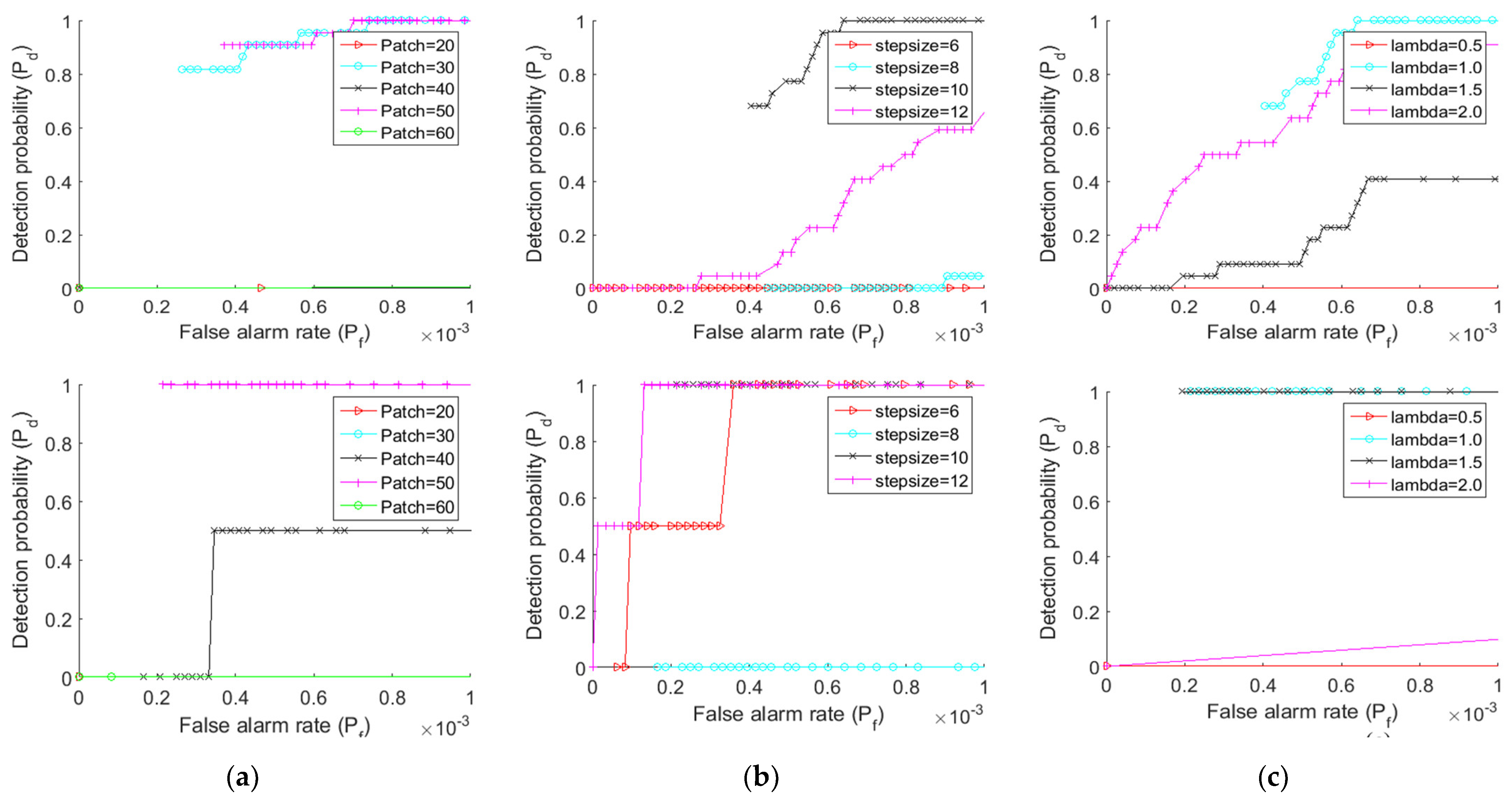
3.4. Parameter Analysis

This section evaluates three critical characteristics that is mainly used to test the robustness of the proposed TV-PSMSV technique under various background scenarios are discussed in the next section. These characteristics are patch size, step size, and regulating parameter. We must use these parameters to achieve greater performance, as they may not provide the global best solution. Evaluation results of Figure 9 shows the ROC curves for four separate images with 4 varying characteristics.

3.4.1. Image Patch-Size

Patch size is thought to be a crucial factor in detection of performance. We know that fine-tuning the patch parameter increases the sparsity of the target. However, this will very certainly increase the computational cost of the method. In the experiment, we tested patch sizes of 20, 30, 40, 50, and 60 and generated the ROC curve for the four image sequences, which can be seen in Figure 9a. The ROC curve shows that adjusting the image patch size had an impact on both detection performance and computational complexity. Patch size 30 is thought to be ideal in the method.

3.4.2. Step-Size

Similarly, the step size must be adjusted properly. In the experiment, the patch size was set to 30 × 30, and then step sizes of 6, 8, 10, and 12 were explored. The ROC curve on step size shows that adopting a small step increases computation time and reduces the algorithm’s detection performance. Reduce calculation time by increasing the step size to a large amount. Figure 9b indicates that a step size of 10 is the optimum option.

3.4.3. Controlling Parameter $\lambda$

The controlling parameter $\lambda =\frac{L}{\sqrt{min\left(m,n\right)}}$ is another key parameter that helps to balance the BPI and TPI. A larger $\lambda$ value would over-shrink the small target, while a small value would leave residue in the complex background image, thereby increasing the number of false alarms. L = 0.5, L = 1, L = 1.5, and L = 2 are the four values we chose for L. Figure 9c shows the experimental results for various L values (c). When compared to various L values, the ideal value at L = 1 yields an excellent performance.

3.4.4. Computational or Running Complexity

Table 4. Comparative summary of time and computing cost.

Method	Top-Hat	Max-Median	Max-Mean	RPCA	NIPPS	IPI	RIPT	TV-PCP	TV-PSMSV
Time (s)	0.868	6.65	7.69	8.77	4.11	11.51	1.93	392.77	242.69
Computational Cost	O (K2 M × N log K)	O (M × N × K2)	O (M × N × K2)	O (M × N2)	O (M × N2)	O (M × N2)	O (M × N2)	O (K × M × N2)	O (K × M × N2)

depicts the running time along with the execution cost of one scene out of the whole dataset as in Figure 2a. The total computation cost of the top-hat method with the size of the structure element as K² and the size of the image as M × N is O (K²logK²MN), whereas the execution cost of the max-mean and max-mean methods here is O (M × N × K²). The execution cost of all competing approaches based on the IPI model is O (M × N²), where the patch image size is M × N and it depends on the cost of the SVD of each step in the algorithm.

The cost for the NIPPS, RPCA,RIPT and IPI is O (m × n²) and for TV-PCP and the finally for proposed TV-PSMSV method, the cost of ADMM to updating every sub problem and the multipliers for running patch size of m × n is O (m × n). In addition, the cost of executing a 2-D TV regularisation is O (m × n log (m × n), while the cost of running a full SVD is O (m × n²). As a result, the total calculation cost is O ((m × n) + (m × n log (m × n) + (m × n)²); in the worst case, the cost will be O (m × n² × k), where k denotes the number of time running the process. Because of the induction of TV regularisation, the suggested TV-PSMSV has a substantially higher cost of running per image than the other baseline approaches due to the introduction of TV regularization.

4. Conclusions

In the present work a model, namely, TV-PSMSV is presented, which is used in the ISTD system. This model addressed the issue of employing NNM for restricting the BPI in existing IPI-based approaches. In TV-PSMSV, NNM was substituted with PSMSV to constrain the BPI due to over-shrinkage of singular values. Secondly, to take care of the strong edges in the background of the input scene and to improve the object of interest, a TV regularisation term was inducted into the BPI. Finally, the ADMM approach was used to solve the target-background separation procedure. Experimental outcome demonstrate that the presented TV-PSMSV method yielded better results in stronger background suppression and detection ability than previous baseline approaches. In the near future, this work can be extended into more robust tensor-patch images-based models to improve existing IPI-based approaches.

References

1. Gao, C.; Meng, D.; Yang, Y.; Wang, Y.; Zhou, X.; Hauptmann, A.G. Infrared Patch-Image Model for Small Target Detection in a Single Image. IEEE Trans. Image Process. 2013, 22, 4996–5009. [Google Scholar] [CrossRef] [PubMed]
2. Chen, C.L.P.; Li, H.; Wei, Y.; Xia, T.; Tang, Y.Y. A Local Contrast Method for Small Infrared Target Detection. IEEE Trans. Geosci. Remote Sens. 2014, 52, 574–581. [Google Scholar] [CrossRef]
3. Reed, I.S.; Gagliardi, R.M.; Stotts, L.B. Optical moving target detection with 3-D matched filtering. IEEE Trans. Aerosp. Electron. Syst. 1988, 24, 327–336. [Google Scholar] [CrossRef]
4. Rawat, S.; Verma, S.K.; Kumar, Y. Review on recent development in infrared small target detection algorithms. Procedia Comput. Sci. 2020, 167, 2496–2505. [Google Scholar] [CrossRef]
5. Bae, T.-W.; Kim, Y.-C.; Ahn, S.-H.; Sohng, K.-I. A novel Two-Dimensional LMS (TDLMS) using sub-sampling mask and step-size index for small target detection. IEICE Electron. Express 2010, 7, 112–117. [Google Scholar] [CrossRef] [Green Version]
6. Deshpande, S.D.; Er, M.H.; Venkateswarlu, R.; Chan, P. Max-mean and max-median filters for detection of small targets. In Signal and Data Processing of Small Targets; SPIE: Denver, CO, USA, 1999; Volume 3809, pp. 74–84. [Google Scholar] [CrossRef]
7. Rawat, S.; Verma, S.K.; Kumar, Y. Infrared small target detection based on Non-convexTriple Tensor Factorization. IET Image Process. 2021, 15, 556–570. [Google Scholar] [CrossRef]
8. Itti, L.; Koch, C.; Niebur, E. A model of saliency-based visual attention for rapid scene analysis. IEEE Trans. Pattern Anal. Mach. Intell. 1998, 20, 1254–1259. [Google Scholar] [CrossRef] [Green Version]
9. Li, G.; Liu, F.; Sharma, A.; Khalaf, O.I.; Alotaibi, Y.; Alsufyani, A.; Alghamdi, S. Research on the Natural Language Recognition Method Based on Cluster Analysis Using Neural Network. Math. Probl. Eng. 2021, 9982305. [Google Scholar] [CrossRef]
10. Alotaibi, Y. A New Database Intrusion Detection Approach Based on Hybrid Meta-heuristics. Comput. Mater. Contin. 2021, 66, 1879–1895. [Google Scholar] [CrossRef]
11. Suryanarayana, G.; Chandran, K.; Khalaf, O.I.; Alotaibi, Y.; Alsufyani, A.; Alghamdi, S.A. Accurate Magnetic Resonance Image Super-Resolution Using Deep Networks and Gaussian Filtering in the Stationary Wavelet Domain. IEEE Access 2021, 9, 71406–71417. [Google Scholar] [CrossRef]
12. Hu, T.; Zhao, J.J.; Cao, Y.; Wang, F.L.; Yang, J. Infrared small target detection based on saliency and principle component analysis. J. Infrared Millim. Waves 2010, 29, 303–306. [Google Scholar]
13. Gao, C.; Su, H.; Li, L.; Li, Q.; Huang, S. Small infrared target detection based on kernel principal component analysis. In Proceedings of the 2012 5th International Congress on Image and Signal Processing, Chongqing, China, 16–18 October 2012; pp. 1335–1339. [Google Scholar]
14. Wang, X.; Shen, S.; Ning, C.; Xu, M.; Yan, X. A sparse representation-based method for infrared dim target detection under sea--sky background. Infrared Phys. Technol. 2015, 71, 347–355. [Google Scholar] [CrossRef]
15. Wang, C.; Qin, S. Adaptive detection method of infrared small target based on target-background separation via robust principal component analysis. Infrared Phys. Technol. 2015, 69, 123–135. [Google Scholar] [CrossRef]
16. He, Y.; Li, M.; Zhang, J.; An, Q. Small infrared target detection based on low-rank and sparse representation. Infrared Phys. Technol. 2015, 68, 98–109. [Google Scholar] [CrossRef]
17. Zhang, Z.; Ren, J.; Li, S.; Hong, R.; Zha, Z.; Wang, M. Robust Subspace Discovery by Block-diagonal Adaptive Locality-constrained Representation. In Proceedings of the 27th ACM International Conference on Multimedia, Association for Computing Machinery (ACM), Nice, France, 21–25 October 2019; pp. 1569–1577. [Google Scholar]
18. Dai, Y.; Wu, Y.; Song, Y. Infrared small target and background separation via column-wise weighted robust principal component analysis. Infrared Phys. Technol. 2016, 77, 421–430. [Google Scholar] [CrossRef]
19. Dai, Y.; Wu, Y.; Song, Y.; Gao, J. Non-negative infrared patch-image model: Robust target-background separation via partial sum minimization of singular values. Infrared Phys. Technol. 2017, 81, 182–194. [Google Scholar] [CrossRef]
20. Guo, J.; Wu, Y.; Dai, Y. Small target detection based on reweighted infrared patch--image model. IET Image Process. 2017, 12, 70–79. [Google Scholar] [CrossRef]
21. Gu, S.; Xie, Q.; Meng, D.; Zuo, W.; Feng, X.; Zhang, L. Weighted Nuclear Norm Minimization and Its Applications to Low Level Vision. Int. J. Comput. Vis. 2017, 121, 183–208. [Google Scholar] [CrossRef]
22. Zhang, L.; Li, M.; Qiu, X.; Zhu, Y. Infrared Small Target Detection Based on Four-Direction Overlapping Group Sparse Total Variation. Trait. Signal 2020, 37, 367–377. [Google Scholar] [CrossRef]
23. Wang, X.; Zhenming, P.; Dehui, K.; Zhang, P.; He, Y. Infrared dim target detection based on total variation regularization and principal component pursuit. Image Vis. Comput. 2017, 63, 1–9. [Google Scholar] [CrossRef]
24. Rawat, S.; Verma, S.K.; Kumar, Y. Reweighted infrared patch image model for small target detection based on non-convex p-norm minimisation and TV regularization. IET Image Process. 2020, 14, 1937–1947. [Google Scholar] [CrossRef]
25. Wan, M.; Gu, G.; Xu, Y.; Qian, W.; Ren, K.; Chen, Q. Total Variation-Based Interframe Infrared Patch-Image Model for Small Target Detection. IEEE Geosci. Remote Sens. Lett. 2022, 19, 1–5. [Google Scholar] [CrossRef]
26. Dai, Y.; Wu, Y. Reweighted Infrared Patch-Tensor Model with Both Nonlocal and Local Priors for Single-Frame Small Target Detection. IEEE J. Sel. Top. Appl. Earth Obs. Remote Sens. 2017, 10, 3752–3767. [Google Scholar] [CrossRef] [Green Version]
27. Zhang, L.; Peng, L.; Zhang, T.; Cao, S.; Peng, Z. Infrared small target detection via non-convex rank approximation minimization joint l2,1 norm. Remote Sens. 2018, 10, 1821. [Google Scholar] [CrossRef] [Green Version]
28. Zhang, L.; Peng, Z. Infrared Small Target Detection Based on Partial Sum of the Tensor Nuclear Norm. Remote Sens. 2019, 11, 382. [Google Scholar] [CrossRef] [Green Version]
29. Rudin, L.I.; Osher, S.; Fatemi, E. Nonlinear total variation based noise removal algorithms. Phys. D Nonlinear Phenom. 1992, 60, 259–268. [Google Scholar] [CrossRef]
30. Chen, G.; Zhang, J.; Li, D.; Chen, H. Robust Kronecker product video denoising based on fractional-order total variation model. Signal Process. 2016, 119, 1–20. [Google Scholar] [CrossRef]
31. Oh, T.-H.; Tai, Y.-W.; Bazin, J.-C.; Kim, H.; Kweon, I.S. Partial Sum Minimization of Singular Values in Robust PCA: Algorithm and Applications. IEEE Trans. Pattern Anal. Mach. Intell. 2016, 38, 744–758. [Google Scholar] [CrossRef] [Green Version]
32. Wang, Z.; Li, H.; Ling, Q.; Li, W. Robust Temporal-Spatial Decomposition and Its Applications in Video Processing. IEEE Trans. Circuits Syst. Video Technol. 2013, 23, 387–400. [Google Scholar] [CrossRef]
33. Donoho, D.L.; Johnstone, I.M. Adapting to Unknown Smoothness via Wavelet Shrinkage. J. Am. Stat. Assoc. 1995, 90, 1200. [Google Scholar] [CrossRef]
34. Hale, E.T.; Yin, W.; Zhang, Y. Fixed-Point Continuation for ℓ1ℓ1-Minimization: Methodology and Convergence. SIAM J. Optim. 2008, 19, 1107–1130. [Google Scholar] [CrossRef]
35. Li, C. An Efficient Algorithm for Total Variation Regularization with Applications to the Single Pixel Camera and Compressive Sensing; Rice University: Houston, TX, USA, 2010. [Google Scholar]
36. Lin, Z.; Chen, M.; Ma, Y. The augmented Lagrange multiplier method for exact recovery of corrupted low-rank matrices. arXiv 2010, arXiv:1009.5055. [Google Scholar]
37. Bai, X.; Zhou, F. Analysis of new top-hat transformation and the application for infrared dim small target detection. Pattern Recognit. 2010, 43, 2145–2156. [Google Scholar] [CrossRef]
38. Hilliard, C.I. Selection of a clutter rejection algorithm for real-time target detection from an airborne platform. In Proceedings of the SPIE Proceedings, Orlando, FL, USA, 13 July 2000; Volume 4048, pp. 74–84. [Google Scholar]
39. Gu, Y.; Wang, C.; Liu, B.; Zhang, Y. A Kernel-Based Nonparametric Regression Method for Clutter Removal in Infrared Small-Target Detection Applications. IEEE Geosci. Remote Sens. Lett. 2010, 7, 469–473. [Google Scholar] [CrossRef]
Figure 1. The proposed TV-PSMSV process.
Mathematics 10 00671 g001
Figure 2. Following rows (ae) depicts the background suppression result on six original image sequences: (a) Original six image sequences (b) Max-mean (c) Max-median and (d) Top-hat (e) IPI.
Mathematics 10 00671 g002
Figure 3. Following rows (ae) depicts the Background suppression result on six original image sequences: (a) RPCA, (b) NIPPS, (c) RIPT, (d) TV-PCP, (e) PSMSV-TV.
Mathematics 10 00671 g003
Figure 4. Target background separation result is presented in column (ae). (a) original images (b) Low rank background (c) sparse target (d) 3-D mesh of (a,e) 3-D mesh of (c).
Mathematics 10 00671 g004
Figure 5. Experimental result in case of noisy images, (a) Real images, (b) Noisy images with standard deviation (sd.) of 10, (c) Background suppression Figure 4b, (d) Noisy images with standard deviation (sd.) of 20, and (e) Background suppression Figure 4d.
Mathematics 10 00671 g005
Figure 6. Experimental result in case of synthetic images, (a) Background, (b) One Target, (c) Result of Figure 5b, (d) Four targets, and (e) Result of Figure 5d.
Mathematics 10 00671 g006
Figure 7. ROC graph of dataset image sequences (ac).
Mathematics 10 00671 g007
Figure 8. ROC graph of dataset image sequences (ac).
Mathematics 10 00671 g008
Figure 9. Experimental result of ROC curve for infrared image sequences 1–4 (a) Results under different patch size (b) Results under different step size. (c) Results under different controlling parameter.
Mathematics 10 00671 g009