
Fractional Euler-Lagrange Equations Applied to Oscillatory Systems


Abstract
:1. Introduction
2. Methodology
2.1. Fractional Euler-Lagrange Equations
2.2. Applications
2.2.1. The Simple Pendulum—Modeling
2.2.2. Spring-Mass-Damper System-Modeling
2.3. Conditions and Parameters of the Simulations

| Simple Pendulum | Spring-Mass-Damper System | |
|---|---|---|
| Case | External force | External force |
| Case A | Q1 = 0 | Q1 = 0 |
| Case B | Q1 = A cos(wt) | Q1 = A cos(wt) |
| Case C | Q1 = A cos (wt) l1 sin (θ) | Q1 = Impulsive function |
| Simple Pendulum | Spring-Mass-Damper System | ||
|---|---|---|---|
| Mass | m = 1kg | Mass | m = 1kg |
| Acceleration of gravity | g = 9.81m/s² | Acceleration of gravity | g = 9.81m/s² |
| Length of the string | l1 = 1m | Stiffness and damping constants | k = 5; c = 0.1 |
| Coefficient tau | τ = 1 | Coefficient tau | τ = 1 |
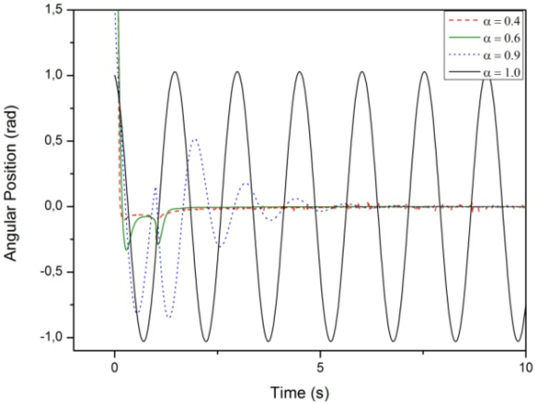
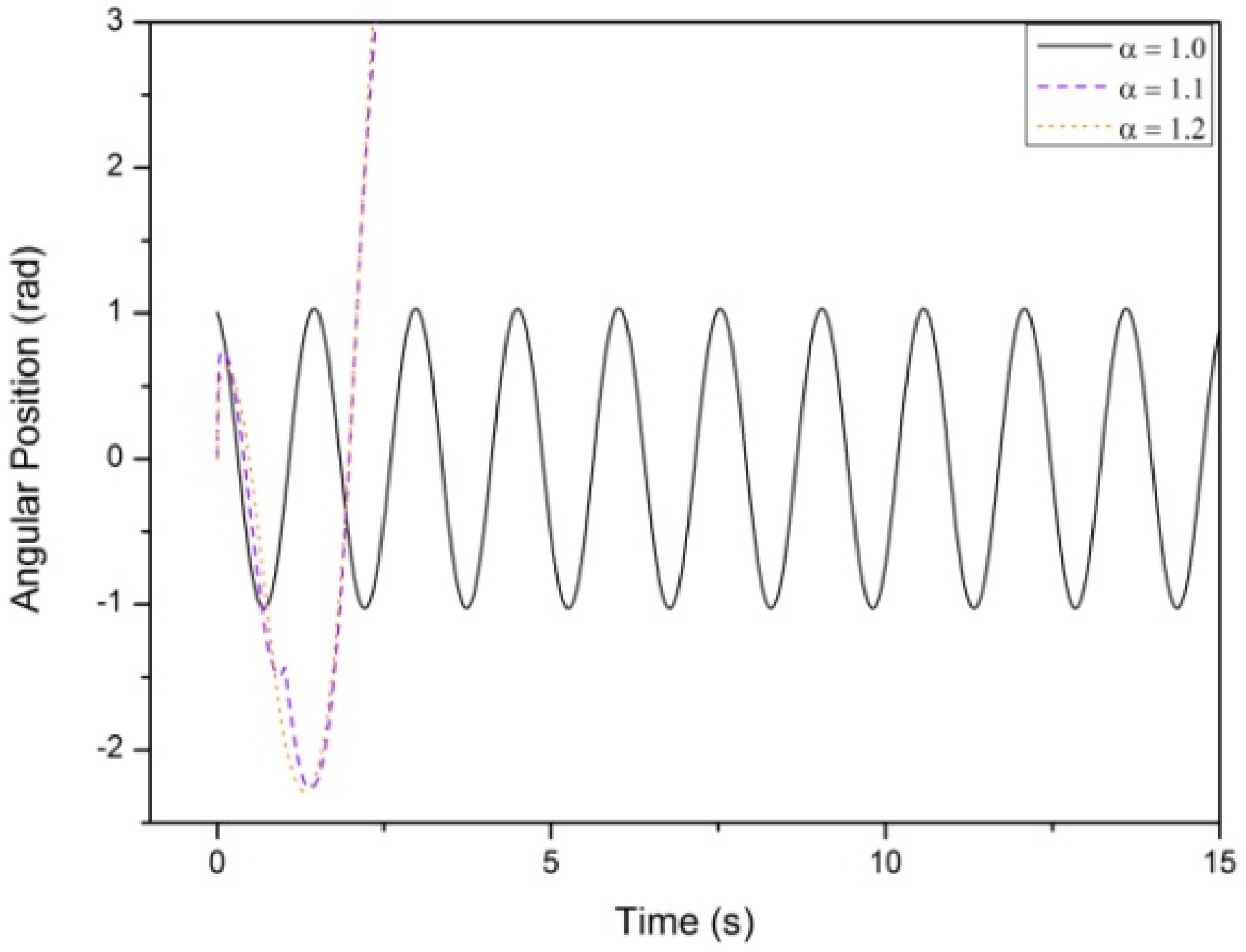
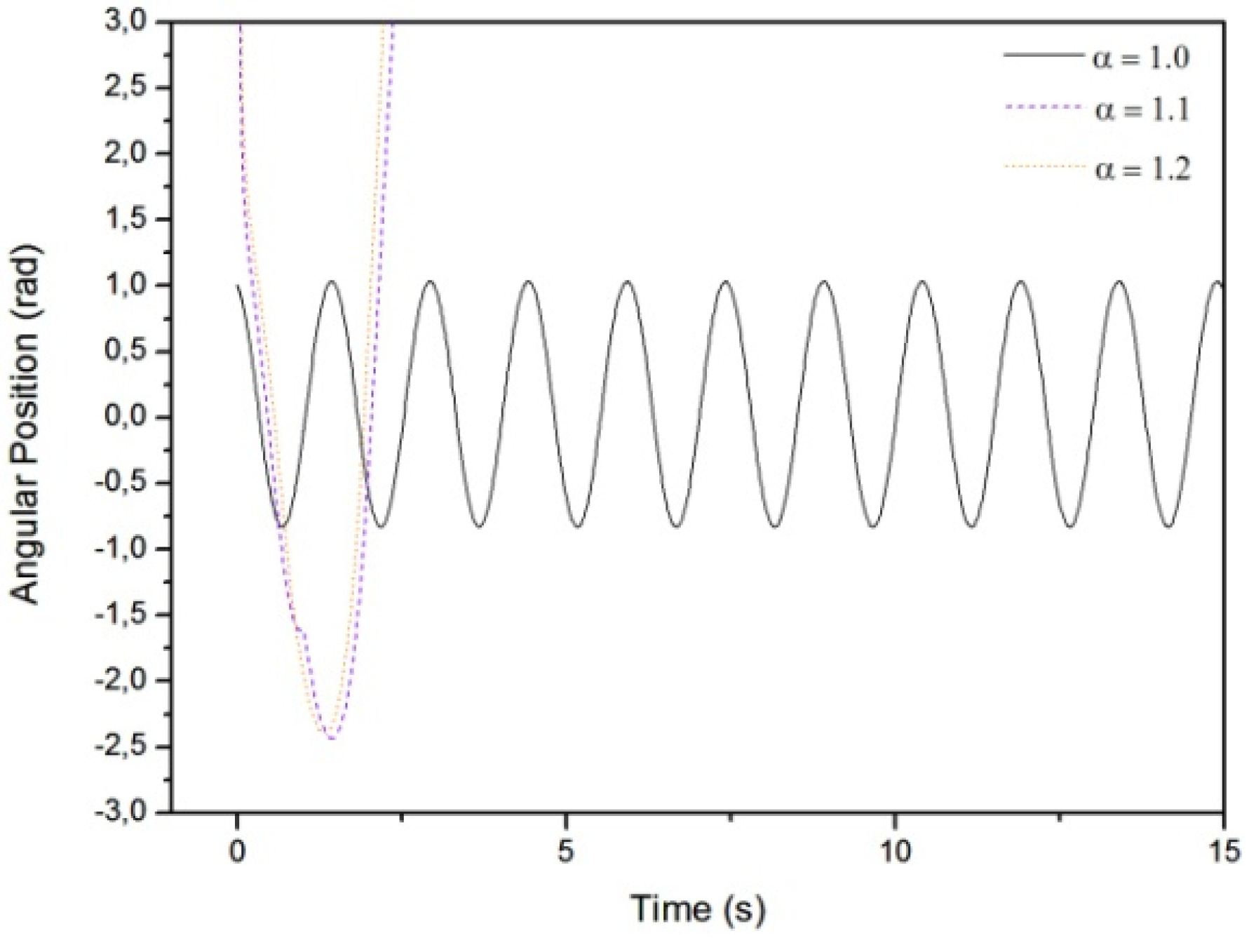
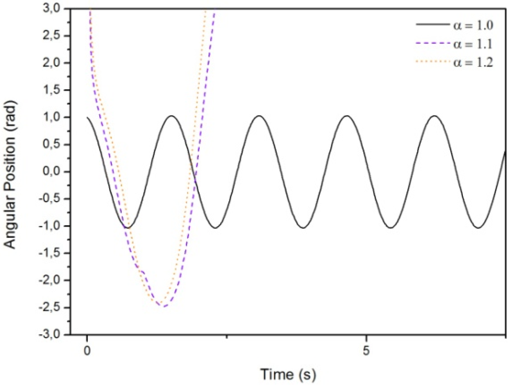
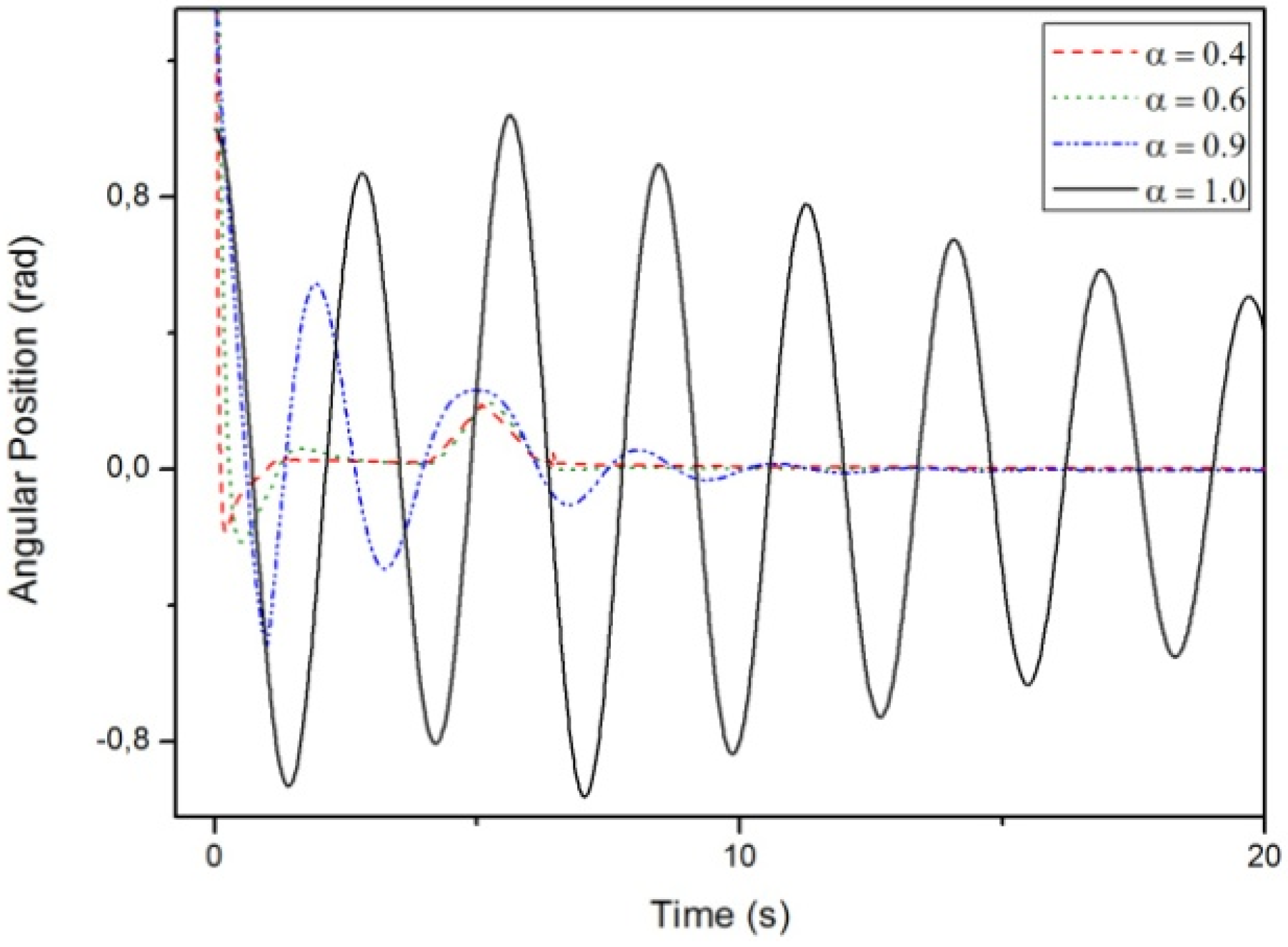
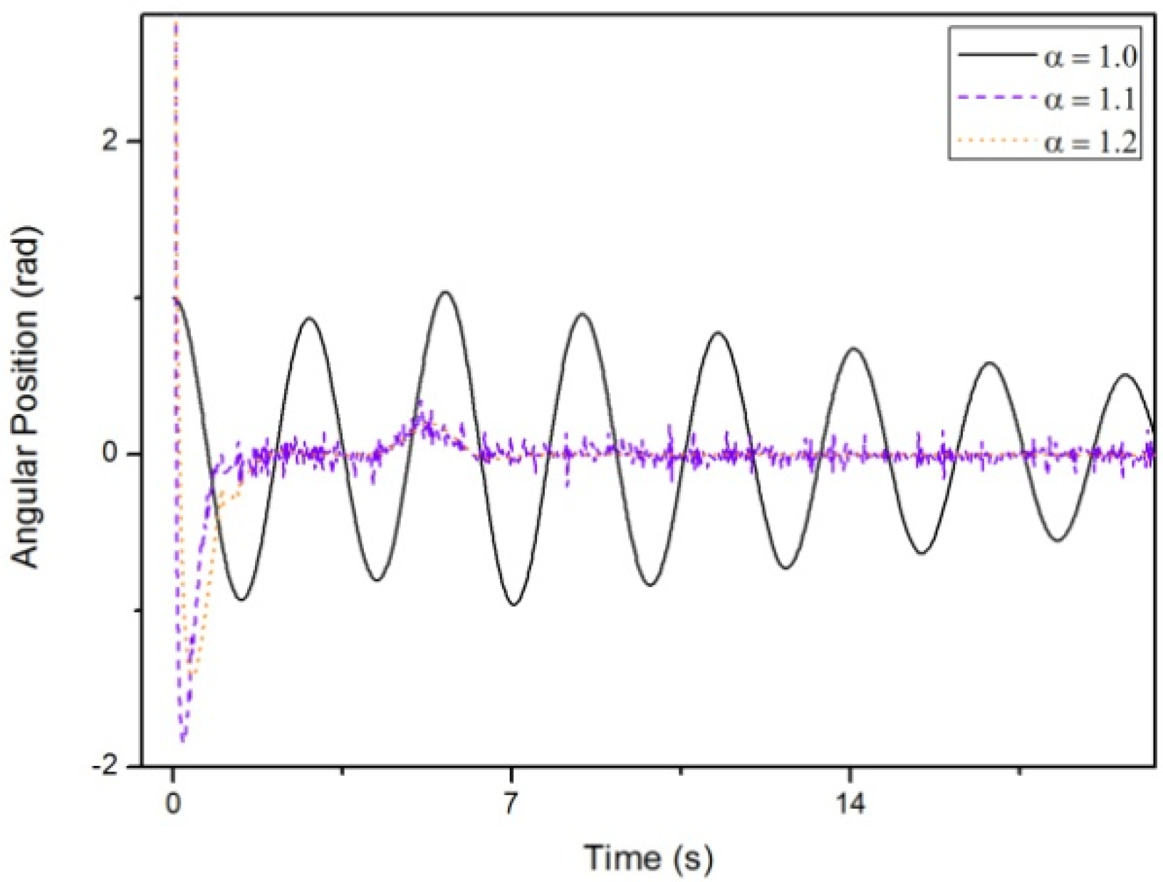
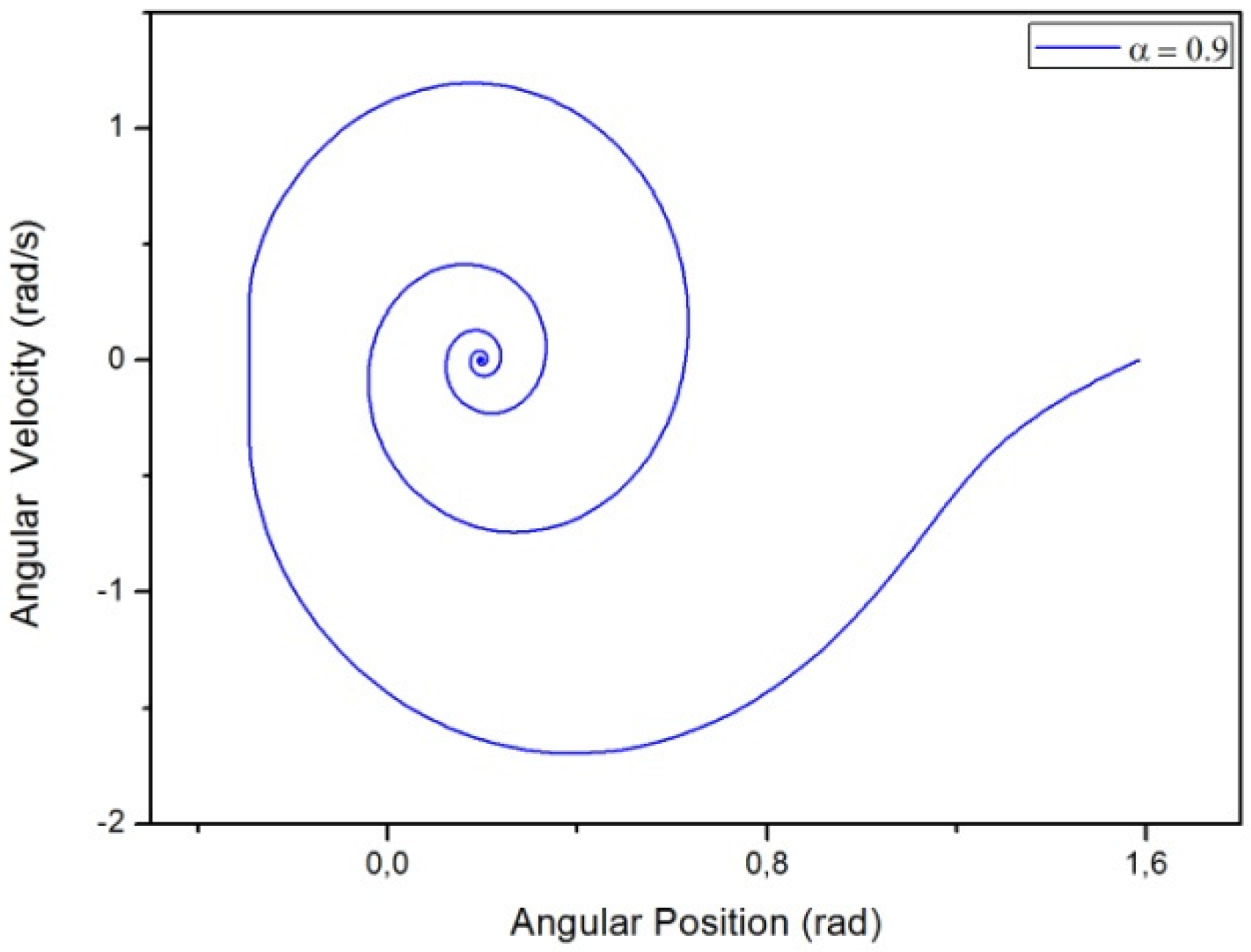
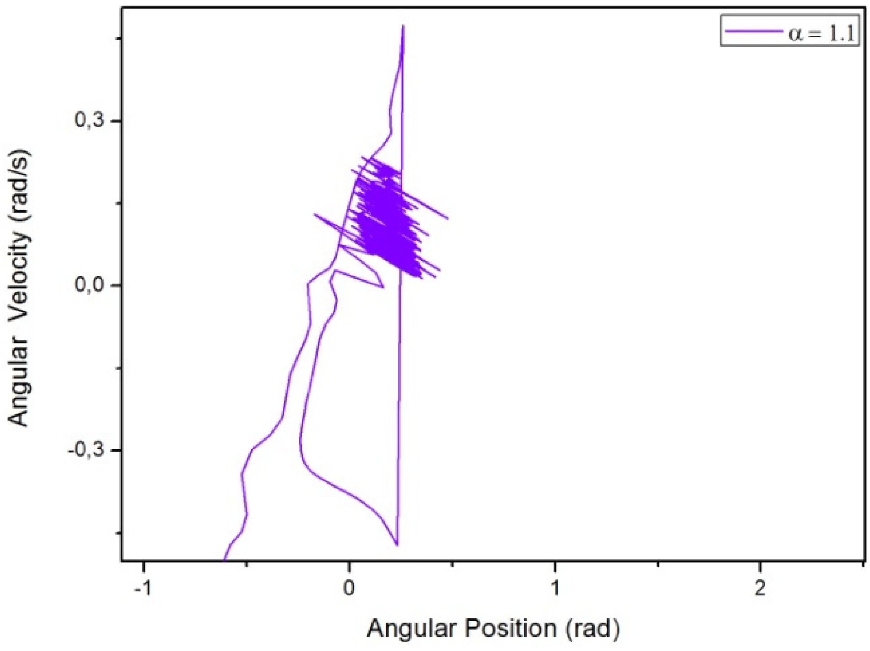
| Coefficient α (with β = α) | τ = 1; α = 0.4; α = 0.6; α = 0.9; α = 1.0; α = 1.1; α = 1.2 | Coefficient α (with β = α) | τ = 1; α = 0.4; α = 0.6; α = 0.9; α = 1.0; α = 1.1; α = 1.2 |
3. Simulation Results
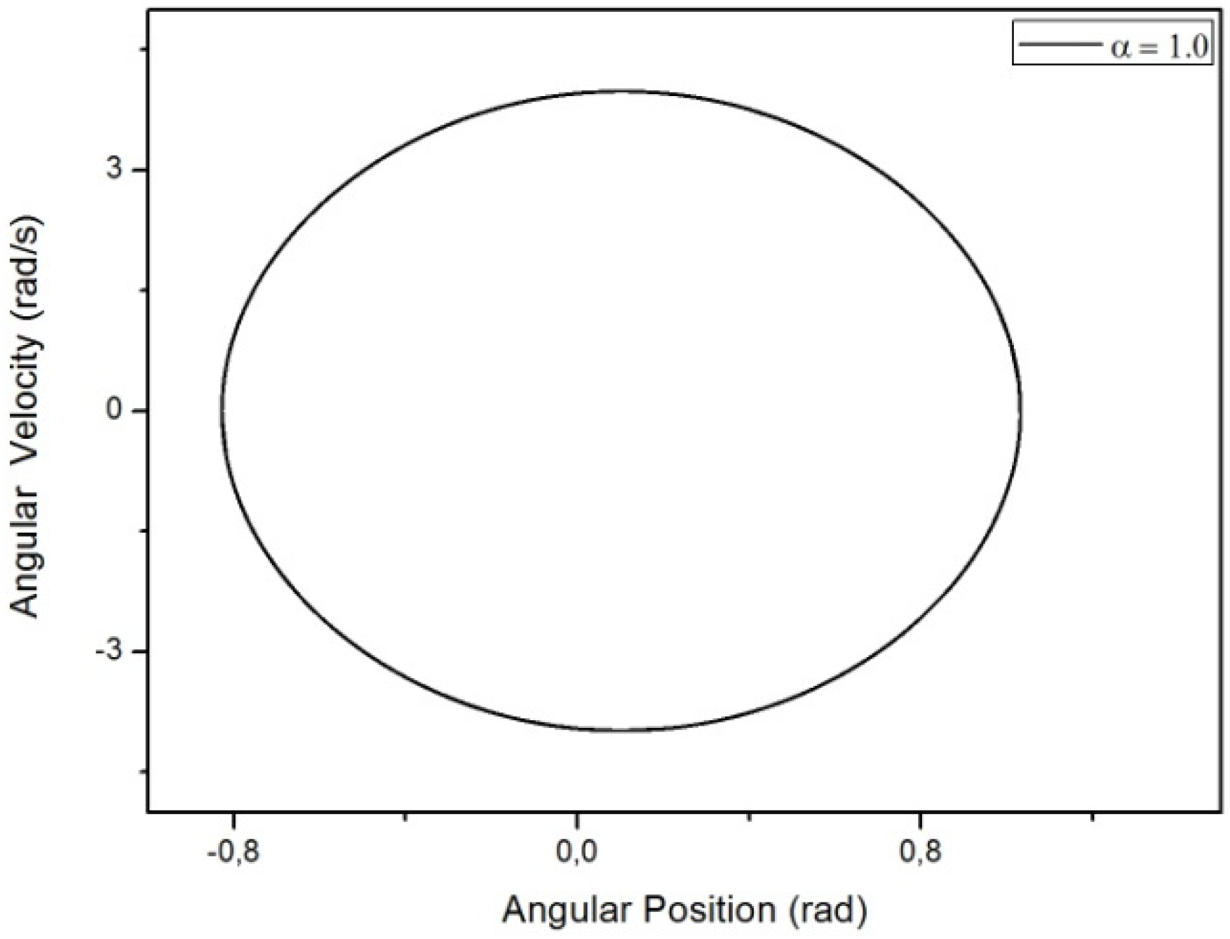
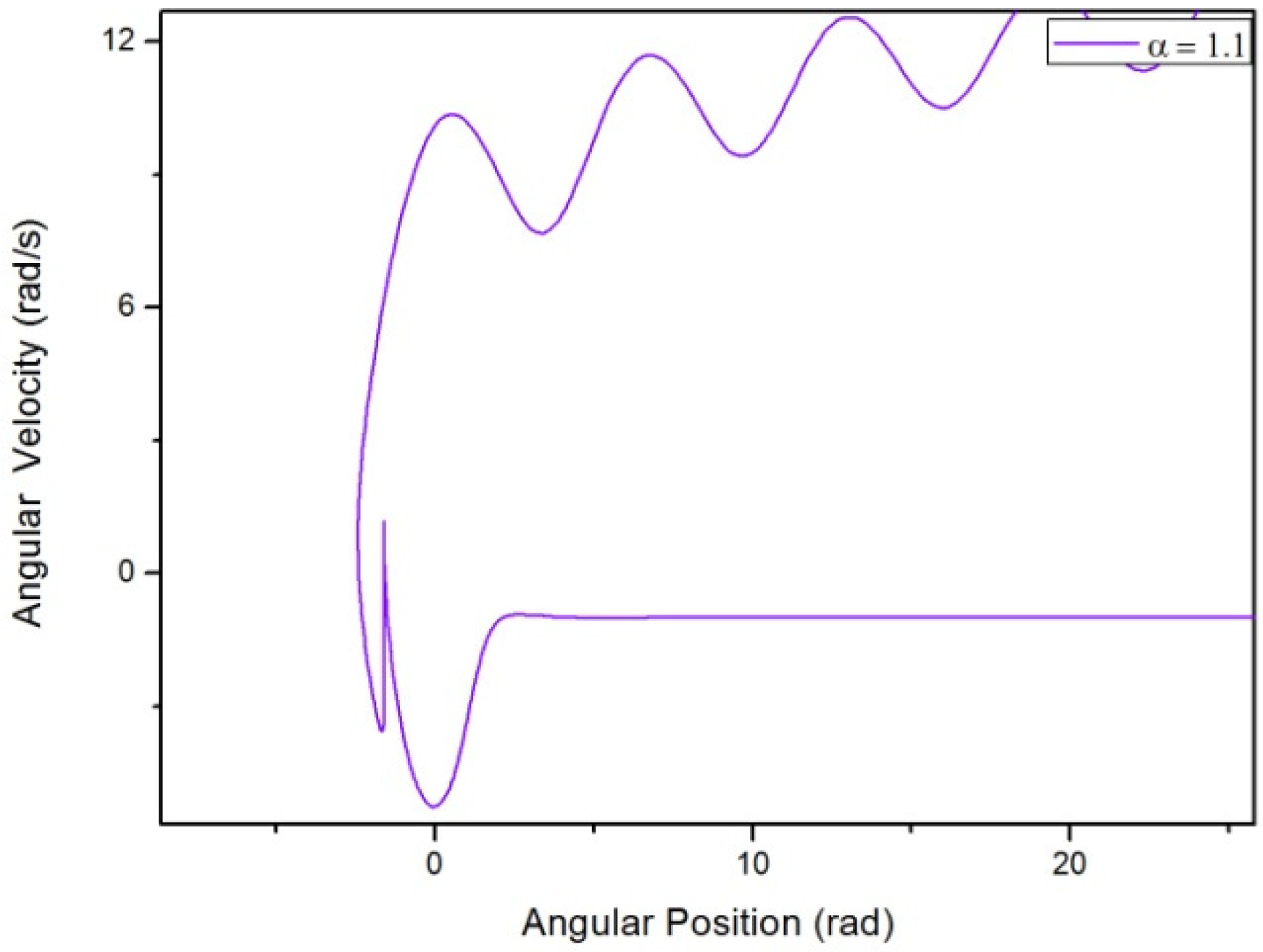
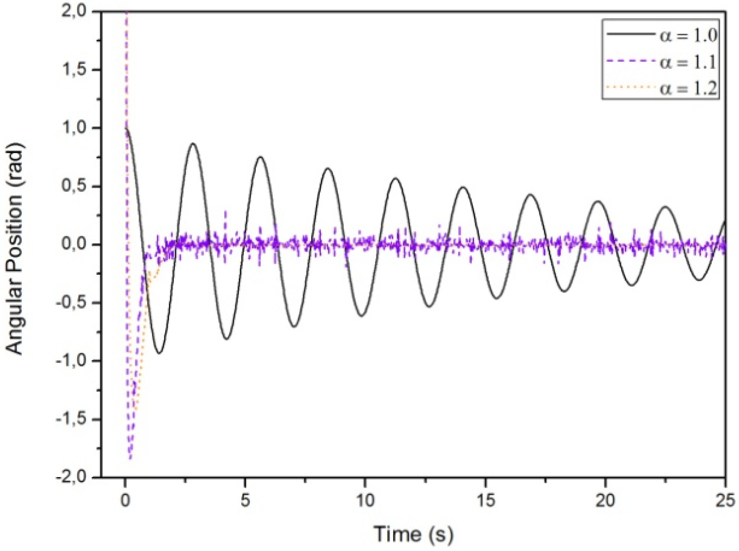
3.1. Results Regarding the Simple Pendulum
- Case A:
- Case B:
- Case C:


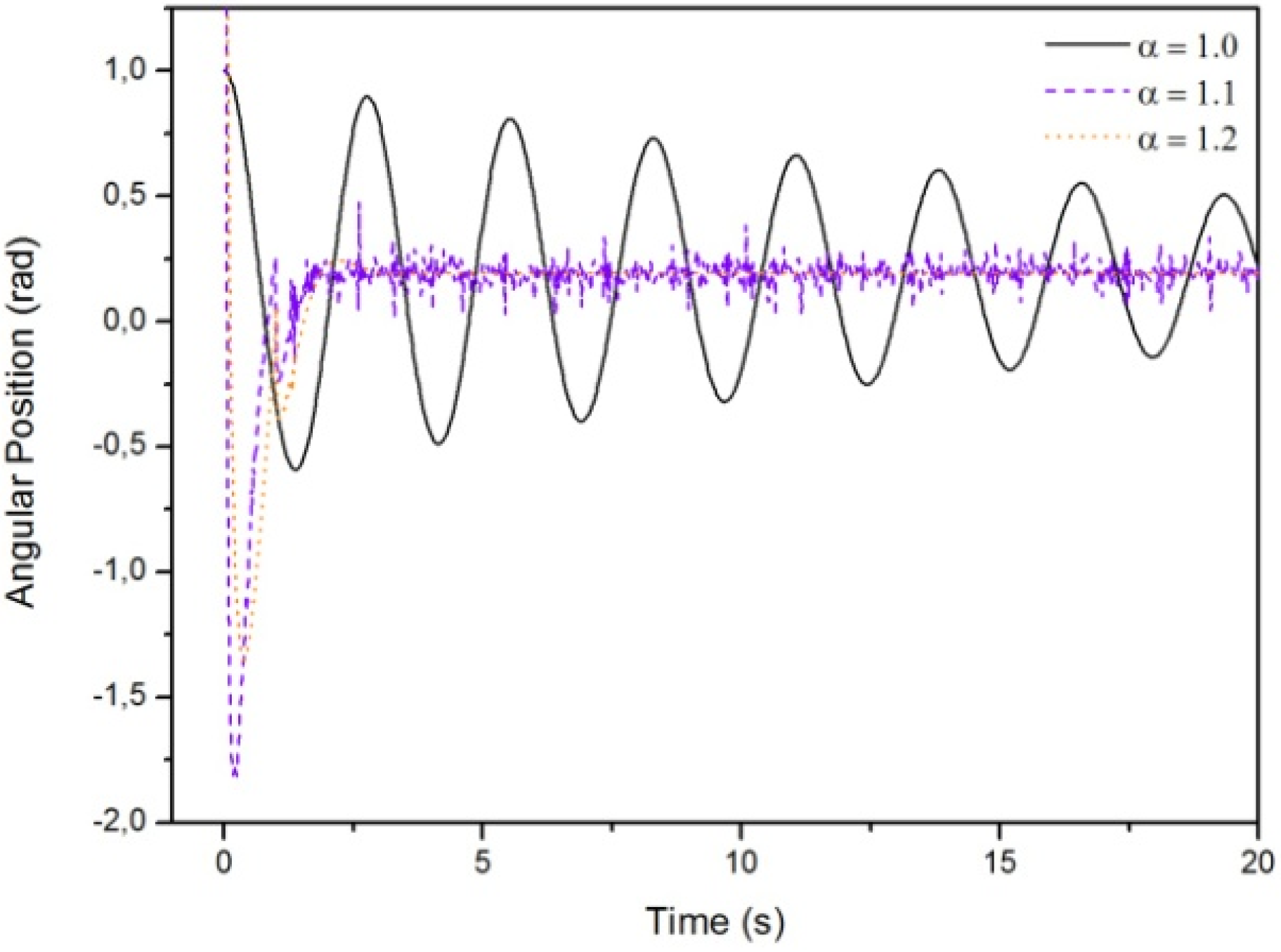
3.2. Results Regarding The Spring-Mass-Damper System
- Case A:
- Case B:
- Case C:


4. Discussion and Conclusions
Acknowledgments
Author Contributions
Conflicts of Interest
References
- Oldham, K.B.; Spanier, J. The Fractional Calculus: Theory and Applications of Differentiation and Integration to Arbitrary Order 1974.
- Kilbas, A.A.; Srivastava, H.M.; Trujillo, J.J. Theory and Applications of Fractional Differential Equations; Elsevier Science Limited: Amsterdam, the Netherlands, 2007; pp. 154–196. [Google Scholar]
- David, S.A.; Linares, J.L.; Pallone, E.M.J.A. Fractional order calculus: historical apologia, basic concepts and some applications. Rev. Bras. Ensino Fís. 2011, 33, 4302–4302. [Google Scholar] [CrossRef]
- Podlubny, I. Fractional Differential Equations; Academic Press: Waltham, MA, USA, 1993. [Google Scholar]
- Balachandran, K.; Trujillo, J.J. The nonlocal Cauchy problem for nonlinear fractional integrodifferential equations in Banach Spaces. Nonlinear Anal. Theory Methods Appl. 2010, 72, 4587–4593. [Google Scholar] [CrossRef]
- Machado, J.A.T.; Kiryakova, V.; Mainardi, F. A Poster About the Old History of Fractional Calculus. Fract. Calc. Appl. Anal. 2010, 13, 447–454. [Google Scholar]
- Valerio, D.; Trujillo, J.J.; Rivero, M.; Machado, J.A.T.; Baleanu, D. Fractional calculus: A survey of useful formulas. Eur. Phys. J. Special Topics 2013, 222, 1827–1846. [Google Scholar] [CrossRef]
- de Oliveira, E.C.; T.Machado, J.A. A Review of Definitions for Fractional Derivatives and Integral. Math. Probl. Eng. 2014, 1–6. [Google Scholar] [CrossRef]
- Ahmad-Rami, E.N. A fractional approach to nonconservative Lagrangian dynamical systems. FIZIKA A 2005, 14, 290–298. [Google Scholar]
- Tarasov, E. T. Fractional variations for dynamical systems: Hamilton and Lagrange approaches. J. Phys. A: Math. Gen. 2006, 39, 8409–8425. [Google Scholar] [CrossRef]
- Baleanu, D.; Avkar, T. Lagrangians with linear velocities within Riemann-Liouville fractional derivatives. Nuovo Cim. 2004, B119, 73–79. [Google Scholar]
- Cresson, J.; Inizan, P. About fractional Hamiltonian systems. Phys. Scr. 2009. T136. [Google Scholar] [CrossRef]
- Agrawal, O.P. Fractional variational calculus and the transversality conditions. J. Phys. A 2006, 39, 10375–10384. [Google Scholar] [CrossRef]
- Muslih, S.M.; Baleanu, D. Fractional Euler-Lagrange Equations of Motion in Fractional Space. J. Vib. Control 2007, 13, 1209–1216. [Google Scholar] [CrossRef]
© 2015 by the authors; licensee MDPI, Basel, Switzerland. This article is an open access article distributed under the terms and conditions of the Creative Commons Attribution license (http://creativecommons.org/licenses/by/4.0/).
Share and Cite
David, S.A.; Valentim, C.A., Jr. Fractional Euler-Lagrange Equations Applied to Oscillatory Systems. Mathematics 2015, 3, 258-272. https://0-doi-org.brum.beds.ac.uk/10.3390/math3020258
David SA, Valentim CA Jr. Fractional Euler-Lagrange Equations Applied to Oscillatory Systems. Mathematics. 2015; 3(2):258-272. https://0-doi-org.brum.beds.ac.uk/10.3390/math3020258
Chicago/Turabian StyleDavid, Sergio Adriani, and Carlos Alberto Valentim, Jr. 2015. "Fractional Euler-Lagrange Equations Applied to Oscillatory Systems" Mathematics 3, no. 2: 258-272. https://0-doi-org.brum.beds.ac.uk/10.3390/math3020258