
The Fractional Orthogonal Difference with Applications

Kooikersdreef 620, 7328 BS Apeldoorn, The Netherlands
Mathematics 2015, 3(2), 487-509; https://0-doi-org.brum.beds.ac.uk/10.3390/math3020487
Submission received: 4 March 2015
/
Revised: 3 June 2015
/
Accepted: 4 June 2015
/
Published: 12 June 2015
(This article belongs to the Special Issue Recent Advances in Fractional Calculus and Its Applications)
Abstract
:This paper is a follow-up of a previous paper of the author published in Mathematics journal in 2015, which treats the so-called continuous fractional orthogonal derivative. In this paper, we treat the discrete case using the fractional orthogonal difference. The theory is illustrated with an application of a fractional differentiating filter. In particular, graphs are presented of the absolutel value of the modulus of the frequency response. These make clear that for a good insight into the behavior of a fractional differentiating filter, one has to look for the modulus of its frequency response in a log-log plot, rather than for plots in the time domain.
1. Introduction
In [1], a comprehensive survey is given about the orthogonal derivative. This derivative has a long, but almost forgotten history. The fractional derivative has also a long history. In [2], these two subjects are combined with the fractional orthogonal derivative. This derivative make use of orthogonal polynomials, both continuous (e.g., Jacobi polynomials) and discrete (Hahn polynomials). In this paper, the theory is applied to functions given for a discrete set of points. We use the fractional difference. Grünwald [3] and Letnikov [4] developed a theory of discrete fractional calculus for causal functions (f (x) = 0 for x < 0). We use the definition defined by, e.g., Kuttner [5] or Isaacs [6]. We show that the definition of Grünwald–Letnikov for the fractional difference is a special case of the definition of the fractional orthogonal difference for the Hahn polynomials for causal functions. Bhrawy et al. [7] use orthogonal polynomials to solve fractional differential equations. However, there formulation of the fractional derivative is entirely different from ours.
In Section 2, we give an overview of some results for the fractional derivative following [2] (Section 2).
In Section 3, the theory of the fractional derivative will be applied with a discrete function, and so, the fractional difference is used as a base for deriving a formula for the fractional orthogonal difference.
In Section 4, the theory of the fractional difference is applied with the discrete Hahn polynomials.
In Section 5, we derive the frequency response for the fractional difference with the discrete Hahn polynomials.
In Section 6, the theory will be applied to a fractional differentiating filter. Analog, as well discrete filters are treated. The theory is illustrated by the graphs of the modulus of the frequency responses.
2. Overview of the Results of the Fractional Derivative
In [2], we find the following formulas for the fractional integral: the Weyl and the Riemann–Liouville transform. In terms of these, we can define a fractional derivative.
Let µ ∈ ℂ with e(µ) > 0. Let f be a function on (−∞,b), which is integrable on bounded subintervals. Then, the Riemann–Liouville integral of order µ is defined as:
A sufficient condition for the absolute convergence of this integral is f (−x) = O (x−µ−ϵ),ϵ>0, x→∞
Similarly, for Re(µ) > 0 and f, a locally-integrable function on (a, ∞), such that f (x) = O (x−µ−ϵ), ϵ>0, x→∞, the Weyl integral of order µ is defined as:
Clearly:
The Riemann–Liouville integral is often given for a function f on [0, b) in the form:
This can be obtained from Equation (1) if we assume that f (x) = 0 for x ≤ 0 (then, f is called a causal function).
The fractional derivatives are defined by the following formulas with Re(ν) < n,n a positive integer and
:
Put W0 = id = R0. Under the assumption of sufficient differentiability and convergence, we have WμWV = Wμ+v, RμRv = Rμ+v for all µ, ν ∈ ℂ and Rn = Dn, Wn = (−1)n Dn.
For Re(ν) < 0, formula Equations (2) and (3) are easily derived, and for Re(ν) > 0, they are definitions. This is under the condition that all derivatives of order less then n + 1 of the function f (x) should exist.
Because we need the Fourier transform of Formulas (2) and (3), we use the following theorem. The proof is in [8] (Chapter 2, Section 7) for the Riemann–Liouville derivative, as well as for the Weyl derivative.
Theorem 1. Let f and g be functions on ℝ for which the Fourier transforms exist and are given by:
If g = Wv [f], then:
Here and in the rest of this paper, zv = evInz with − π < arg (z) < π. Therefore, (−iw)v =(−iw+0)v = e−πiv/2(w+i0)v. If z is on the cut (−∞, 0] and z ≠ 0, then we distinguish between (z+i0)v=eiπv(−z)v and (z−i0)v=e−iπv(−z)v
The quotient
will be called the frequency response, where we follow the terminology of filter theory.
In [1], the following theorem is proven:
Theorem 2. Let n be a positive integer. Let pn be an orthogonal polynomial of degree n with respect to the orthogonality measure µ for which all moments exist. Let x ∈ ℝ. Let I be a closed interval, such that, for some ε > 0, x + δu ∈ I, if 0 ≤ δ ≤ ε and u ∈ supp(µ). Let f be a continuous function on I, such that its derivatives of order 1, 2,…, n at x exist. In addition, if I is unbounded, assume that f is of at most polynomial growth on I. Then:
where:
From this formula, with f absolutely integrable on ℝ and
, we immediately derive for the frequency response
:
3. The Fractional Orthogonal Difference
In this section, we treat the fractional difference. If we want to compute the fractional derivative of a function given at a set of equidistant points, we can use instead of the fractional derivative, the fractional difference. Then, we have to work in the formula for the orthogonal derivative with discrete orthogonal polynomials.
As an analog of the Riemann–Liouville fractional integral Equation (1), we can define a fractional summation (see, for example, [5] or [6]) as:
In contrast to the Riemann–Liouville fractional integral, this summation has no a priori singularity for µ < 0. If f is a causal function, then the upper bound for the summation should be [x/δ], and the sum is certainly well-defined. For µ ≠ 0,− 1,− 2,…, we can write:
as k → ∞. Hence, the infinite sum converges if
as x → ∞ with λ > Re(µ). For µ = −n(n a nonnegative integer), we get:
where:
Note that:
More generally, we have:
For µ > 0, the fractional summation
formally approximates the Riemann–Liouville integral R−µ [f]. Indeed, putting y = kδ, we can rewrite the formula for
as:
Formally, we have:
with gδ (y) → g (y) as δ ↓ 0. Application of Equations (8) and (9) to Equation (7) yields:
This is the fractional integral of Riemann–Liouville. Therefore, it is shown that the fractional difference formally tends to the fractional integral in the limit as δ ↓ 0.
Remark 1. Grünwald [3] and Letnikov [4] developed a theory of discrete fractional calculus for causal functions (f (x) = 0 for x < 0). For a good description of their theory, see [10]. They started with the backwards difference:
and next, they define the fractional derivative as:
where. This definition has the advantage that ν is fully arbitrary. No use is made of derivatives or integrals. The disadvantage is that computation of the limit is often very difficult. However, it can be shown that Equation (11) is the same as the Riemann–Liouville derivative for causal functions for Re(ν) > 0 and f is n times differentiable with n > Re(ν). At least formally, this follows also our approach if we write and then use Equation (10) and the fact that Equation (6) approaches the derivative as δ ↓ 0.
Comparing Equation (11) with Equation (5), the differences are the upper bound and the limit. For practical calculations, Formula (11) is often used without the limit. In the next section, we will develop the fractional orthogonal difference for the Hahn polynomials. In Section 5, we will see that the definition of Grünwald–Letnikov for the fractional difference is a special case of the definition of the fractional orthogonal difference for the Hahn polynomials for causal functions.
For obtaining the formula for the fractional orthogonal difference, we let
be a system of orthogonal polynomials with respect to weights w (j) on points j (j = 0, 1,…, N). Then, the approximate orthogonal derivative [2] (3.1b) takes the form:
Let Re(ν) < n with n a positive integer. The fractional derivative
can be formally approximated by:
as δ ↓ 0. This is a motivation to compute
more explicitly, in particular for special choices of the weights w. Substitution of Equations (5) and (12) in Equation (13) gives:
For the double sum, we can write:
Application of this formula to Equation (14) yields:
The summations inside the square brackets are in principle known after a choice of the discrete orthogonal polynomials pn (x). Then, this formula can be used for approximating the fractional orthogonal derivative.
Remark 2. When taking the Fourier transform of the fractional summation, one can show that for δ ↓ 0, this Fourier transform formally tends to the Fourier transform of the fractional integral. For this purpose, we write Equation (5) as:
Taking the discrete Fourier transform gives:
while working formally, we interchange the summations on the right. This gives:
The first summation is well known. We obtain:
Multiply both sides with δ, and take the formal limit for δ ↓ 0. We obtain the well-known formula:
4. The Fractional Orthogonal Difference for the Discrete Hahn Polynomials
In this section, we substitute the discrete Hahn polynomials Qn(x;α,β,N) in Formula (14) to calculate the fractional difference. We do this analogously to Jacobi polynomials in [2]. For the Hahn polynomials, we use the definition in [11]. They give:
For the Hahn polynomials, there are the following properties with n = 0,1, ,…, N:
To compute the sums in Equations (19) and (20), we use partial summation. The general formula for partial summation is:
In particular, if f (N) = f (−1) = 0, then:
Applying this formula n times and remarking that f (N − n) = f (−1) = 0 gives:
For the second fraction inside the summation, we use [12] (Appendix I.(30)) ):
Then, it follows:
For the third fraction inside the summation, we use the formula:
Then, we obtain:
After substitution in J1 (m), we get:
Then, J1 (m) can be written as a hypergeometric function:
Observing the hypergeometric function, we will see that this function represents a series with a finite number of terms (if β is not an integer with − N − β ≠ 0). With α = β = 0 and Re (α) < m, it follows:
Observing the hypergeometric function, we will see that this function represents an infinite series. To compute J2 (m), we write Formula (20) with Equation (17) as:
Suppose:
Then, we rewrite the formula for the partial summation Equation (22) as:
In particular, if f (N — m) = g (−1) = 0, then:
Applying this formula n times gives:
Substitution in Equation (26) gives:
For the ∇ function, we use Formula (24). We obtain:
After substitution in J2 (m), we get:
For j = 0, the factor (m − n + 1) could be less than or equal to zero. Then, the terms concerning this condition should not be taken. In this case, the summation should be reversed. We set j = N − m − i. This gives:
After some manipulations with the Pochhammer symbols, J2 (m) can be written as a hypergeometric function.
With α = β = 0, it follows again, after some manipulations of the Pochhammer symbols:
It can be shown that the hypergeometric function represents a finite series. Then, with [9] (16.4.11), we can rewrite the hypergeometric function. This results in:
Remark 3. To see what conditions are necessary for the given function f (x), so that the first summation is convergent, we split up this summation into two summations:
with:
The hypergeometric function can be summed. There remains:
so for convergence of approximate fractional difference, the summation in Equation (28) should converge.
For α = β = 0, there remains:
For n = 1, it follows:
The first hypergeometric function can be written as:
For the second hypergeometric functions, it is yielded:
After substitution in Equation (29), there remains:
5. The Frequency Response for the Approximate Fractional Orthogonal Difference
Just as for the fractional orthogonal derivative, it is possible to compute the frequency response for the fractional orthogonal difference. In that case, we can apply Theorem 1, where we take another function for the function g. In this case, we use Equation (5):
Fourier transform of this function gives:
The summation is known, and it follows:
For the Hahn polynomials, this becomes:
Substitution in Equation (32) gives:
Substitution of Equation (16) yields:
Comparing this formula with [2] (5.28), we will see that the only difference between these formulas is the factor
. In the next section, we will discuss this fact.
With α = β = 0 and n = 1, there remains:
For N = 1, there remains:
Remark 4. Note that the frequency response in Equation (33) is derived with a summation to infinity. For practical reasons, one should take the summation to a finite number, say M. Then, we have to use the frequency response corresponding to Equation (30). This is important, because Equation (30) is the formula to compute the approximate fractional Hahn derivative. Then, the frequency response will differ from the ideal one. Taking the Fourier transform, the result for the frequency response is:
If f (x) is causal, then Equation (33) can be derived from a finite sum, and we do not cut offthe summation. Then, we can use the frequency response Equation (33) instead of Equation (35).
Remark 5. For the filter for the fractional differentiation of Grünwald and Letnikov, the approximate frequency response (with N finite) can be simply derived from Equation (11) by taking the Fourier transform. We first take the Fourier transform of Equation (11) without the limits. This gives: with N = [x/δ]
Because f (x) is a causal function, it follows that x ≥ kδ. Substitution gives:
For δ → 0, the frequency response becomes:
Because of Section 3.11 from [1], the Grünwald-Letnikov derivative follows by taking w (j) = 1 and N = n in Equation (12) or α = β = 0 and N = n in Equation (15). Therefore, Equation (36) becomes a special case of Equation (33).
6. Application of the Theory to a Fractional Differentiating Filter
This section treats the application of the fractional derivative in linear filter theory. In that theory, a filter is described by three properties, e.g., the input signal, the so-called impulse response function of the filter and the output signal. These properties are described in the time domain. The output signal is the convolution integral of the input signal and the impulse response function of the filter. The linearity means that the output signal depends linearly on the input signal.
One distinguishes between continuous and discrete filters, corresponding to continuity and discreteness, respectively, of the signals involved. In the discrete case, the output signal can be computed with a discrete filter equation.
In the usage of filters, there are two important items for consideration. The first item is the computation of the output signal given the input signal. The second item is a qualification of the working of the filter.
In our opinion, this second task should be preferably done in the frequency domain, where one can see the spectra of the signal and eventually the noise. In this domain, one obtains the Fourier transform of the output signal by multiplication of the Fourier transform of the input signal with the frequency response.
In this section, we will give graphs of the absolute value of the frequency response associated with various approximate fractional derivatives introduced in this paper. From these graphs, we will get insight into how these approximations will work in practice. We think this kind of analysis, in particular when using log-log plots, is preferable to the analysis of filters in the time domain. As an example of the latter type of analysis, actually for the fractional Jacobi derivative, see a paper of Tenreiro Machado [14].
For the second item, the frequency response of the filter should be computed. We treat here the approximate fractional Jacobi derivative and the approximate fractional Hahn derivative. For practical computations, these become the approximate fractional Legendre derivative and the approximate fractional Gram derivative.
For the first item, we can use [2] (4.18) for the Jacobi derivative and [2] (4.39) for the Hahn derivative. For the second item, we had to go to the frequency domain.
In the frequency domain, we suppose that the Fourier transforms of the input signal x (t) and the output signal y (t) are X (ω), and Y (ω) and does exist. The Fourier transformation of the impulse response function h (t) of the filter is the frequency response H (ω) of the filter. For this frequency response, there is the definition:
The function H (ω) is a complex function. For a graphic display of this function, one uses the modulus and the phase of the frequency response. In our case, we want to see the property of the differentiation, and then, the graph of the modulus of the frequency response is preferred.
For an n-th order differentiator, one can show:
In the frequency domain, the graph of the modulus of the frequency response of this filter is a straight line with a slope that depends on n. See Figure 1.
We see that for ω→∞, the modulus of the frequency response |H (ω) | goes to ∞. This means that (because every system has some high-frequency noise) this filter is unstable. That is the reason why a differentiating filter should always have an integrating factor. This factor will be added to the filter, so that for ω→∞, the modulus of the frequency response goes to zero. The filter for the orthogonal derivatives has this property. These derivatives appear from an averaging process (least squares), and such a process will always give an integrating factor.
The formula for the frequency response of the approximate Legendre derivative is [1] (Section 5):
where the functions jn are the spherical Bessel functions [9] (10.49.3). The graph of the modulus of the first order approximate Legendre derivative with δ = 1 is given in Figure 2.
It is clear that for large ω, the modulus of the frequency response goes to zero. For small ω, the graph is a straight line with slope one. In the case that the order of the differentiating filter is not an integer, the formula of the frequency response should be analogous to Equation (37):
where υ can be an integer, a fractional or even a complex number. The graph of the modulus of the frequency response is given in Figure 3.
Furthermore, in this case, there is an instability. To prevent this instability, one can use an approximate fractional Jacobi differentiating filter. For the approximate Jacobi derivative, the frequency response is already computed in [2] (Section 5). We repeat the formula [2] (5.5).
With δ = 1, the squared absolute value of the frequency response of the approximate fractional Jacobi derivative can be written as a series expansion as follows:
For small ω, a first approximation of the modulus of the frequency response gives:
It is clear that the formula is symmetric in α and β. The choices of α and β detect the cut-off frequency For simplicity, we look at the frequency (and not at the exact cut-off frequency) where the frequency response has a first maximum. From Formula (38), the maximum frequency is:
To simplify this formula, set α = β. Then, there remains:
The shape of the curves does not change in principle. Therefore, if one wants the cut-off frequency as high as possible, then α and β should be chosen as high as possible. For the case α = β = 0, the formula for the frequency response of the approximate fractional Jacobi derivative simplifies to the approximate fractional Legendre derivative:
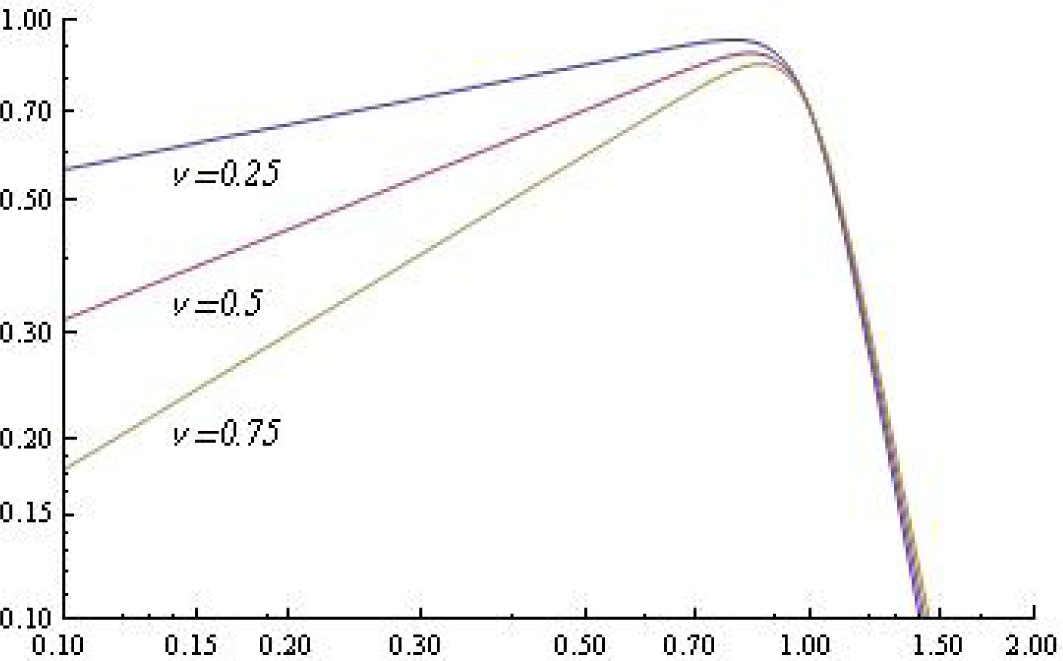
where the functions jn are the spherical Bessel functions with n − 1 ≤ υ ≤ n. For n = 1 and δ =1, there remains:
The graph of the modulus of this frequency response is given in Figure 4 for different values of υ.
Next, we treat the discrete filter.
When we apply a discrete filter, the input signal and the output signal are sampled with a sample frequency that is higher than twice the maximum frequency of the input signal. Therefore, there is always a maximum frequency for the frequency response of the filter. What the frequency response will do above this maximum frequency is not important, presupposing that for ω →∞, the frequency response will go to zero. The input signal is known over N points. Therefore, the input signal is an approximation of the true input signal.
The output signal can be computed for the N points of the input signal. This is the reason that the output signal is always an approximation of the filtered true input signal. If the filter is a differentiator, the output signal is an approximation of the derivative of the input signal. This approximation is very dependent on N.
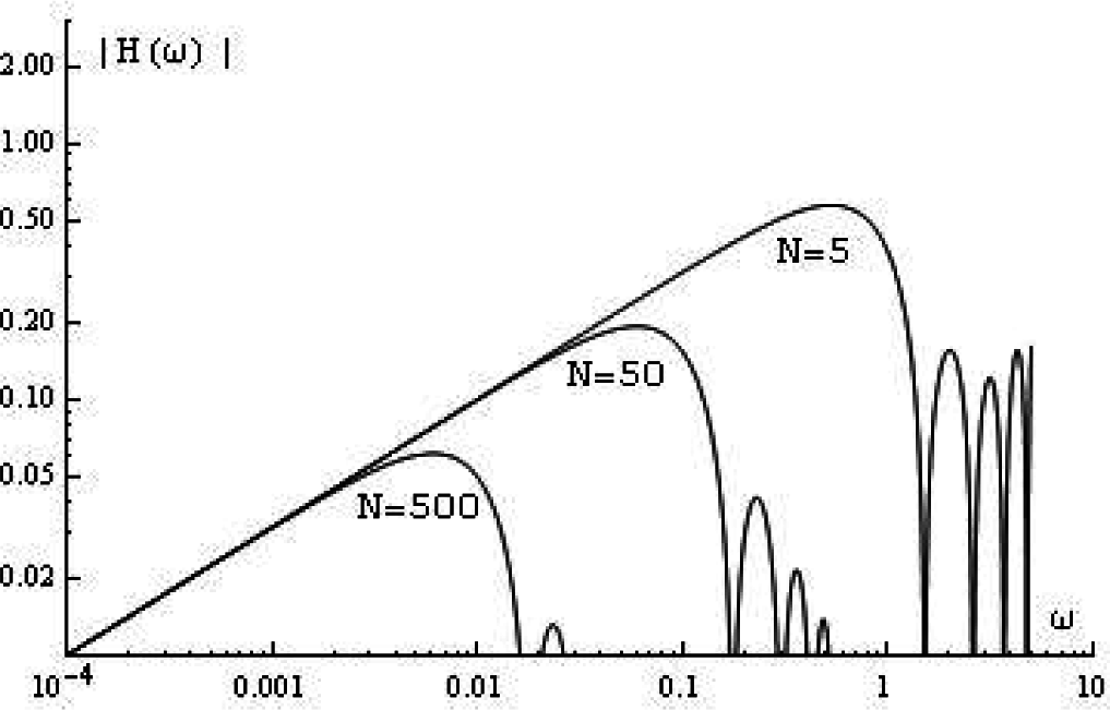
For the fractional orthogonal derivative, we use the frequency response of the approximate derivative of the discrete Hahn difference as derived in Equation (33). For α = β = 0, this frequency response becomes that of the fractional Gram derivative. In the following figure, we take with 0 < υ ≤ 1 and n = 1 in Formula (34). For N = 1, the modulus of the frequency response of the ideal filter has a maximum at ω = π. For different values of N, the modulus of the frequency response with δ = 1 is given in Figure 5.
In practice (taking a finite number of points), we use the frequency response in Equation (35). For δ =1, υ = 0.5, N = 7 and different values of M, the modulus of this frequency response is shown in Figure 6.
We see that for ω → 0, the absolute value of the frequency response tends to a constant value. Taking ω = 0 in Equation (35), it follows:
For the summations, it is proven:
Then, there remains:
The lower bound of the frequency for which the filter does a fractional differentiation can be defined with the help of the following equation:
In practice, we should take this frequency 10-times higher than computed with Equation (40).
For the maximum frequency, we should compute the value of the frequency for the first maximum of the absolute value of Equation (35). A tedious computation leads to:
Therefore, we can define a bandwidth B of the filter, which is equal to B = ωmax – ωl.
For M →∞, we had to take the limits for the ratios of the gamma functions. The work in [9] (5.11.13) gives:
Because ν > 0, this constant goes to zero, and the frequency response approximates the ideal case for low frequencies.
With this frequency response, it is seen that the filter works only well when the frequencies of the input signal lie inside the band-pass of the filter. The maximum frequency of this band-pass is mainly dependent on the number N and the minimum frequency on the number M.
Many authors (e.g., [15–18]) tried to describe the properties of a discrete fractional filter in the time domain with causal functions. Then, there are always transient effects at the initial time t = 0. There, the filter has other properties than elsewhere, because of the discontinuity of the input signal (and the resulting high frequencies).
When using the frequency response, the realms of lower and of higher frequencies need special attention. For the lower frequencies, the frequency response does not go to zero when using a finite number of points (in practice, this is always the case). This we call the minimum frequency effect. When the input signal is causal, the frequency response has no minimum frequency effect (this is important when, for example, treating differential equations). For the higher frequencies, there is always a maximum depending on the sample frequency (Shannon frequency). However, for the orthogonal derivative, there is an extra maximum that is lower than the Shannon frequency. For the GL filter, there is no such maximum.
7. Conclusions
The first conclusion of this paper is that when using a discrete fractional filter, the properties of the filter should be examined using the frequency response. The second conclusion is that a discrete fractional differentiating orthogonal filter has always a certain bandwidth.
In general, a fractional differentiating filter can be built from two serial filters. The first one has a frequency response with modulus |ω|υ. The second filter is a so-called low-pass filter. This low-pass filter determines the highest frequency for differentiation of the filter. In the case of the Jacobi filter (continuous case), one has to keep in mind that the frequency response has side lobes. In the discrete case, these side lobes are not important, because there is a maximum sample frequency. The Jacobi filter can be used if the maximum signal frequency is far beyond the side lobes. These sides lobes go to zero for high frequencies. Hence, this is a very good fractional differentiating filter.
As another example for the low-pass filter, we can choose the Butterworth filter. For this filter, the frequency response is:
which gives a very good frequency response for fractional differentiation. There are no side lobes. In Figure 7, this is demonstrated. There is no simple analogous discrete filter.
The work in [1] makes some remarks about the practical applications of the filters obtained from orthogonal polynomials and the Butterworth filter. In the analog integer case, the Butterworth filter can be much more easily constructed physically In the analog fractional case, a filter should be built with the frequency response (−iω)υ. This gives a difficult problem. Solutions are always approximations.
In the discrete case, the Butterworth frequency response can be transformed into a filter equation. See [19]. For more details about the Butterworth filter, see [20] (Section 5.2.1) (both analog and discrete), [21] (both analog and discrete), [22] (Section 3.2) (analog) and [19] (Section 12.6) (digital).
Acknowledgments
I thank T.H. Koornwinder for his help and time offered during my writing of this paper. Especially his hints about the Hahn polynomials were very helpful. Without his very stimulating enthusiasm and everlasting patience, this work could not be done.
References
- Diekema, E.; Koornwinder, T.H. Differentiation by integration using orthogonal polynomials, a survey. J. Approx. Theory 2012, 164, 637–667. [Google Scholar]
- Diekema, E. The fractional orthogonal derivative. Mathematics 2015, 3, 273–298. [Google Scholar]
- Grünwald, A.K. Ueber “begrenzte” Derivationen und deren Anwendung. Z. Math. Phys. 1867, 12, 441–480. [Google Scholar]
- Letnikov, A.V. Theory of Differentiation of Fractional Order. Mat. Sb. 1868, 3, 1–68. [Google Scholar]
- Kuttner, B. On differences of fractional order. Proc. Lond. Math. Soc. 1957, 34–7, 453–466. [Google Scholar]
- Isaacs, G.L. An iteration formula for fractional differences. Proc. Lond. Math. Soc. 1963, 3, 430–460. [Google Scholar]
- Bhrawy, A.H.; Zaky, M.A. A method based on the Jacobi tau approximation for solving multi-term time-space fractional partial differential equations. J. Comput. Phys. 2015, 281, 876–895. [Google Scholar]
- Samko, S.G.; Kilbas, A.A.; Marichev, O.I. Fractional Integrals and Derivatives; Gordon and Breach: Newark, NJ, USA, 1993. [Google Scholar]
- Olver, F.W.J.; Lozier, D.W.; Boisvert, R.F.; Clark, C.W. NIST Handbook of Mathematical Functions; Cambridge University Press: Cambridge, UK, 2010. [Google Scholar]
- Oldham, K.B.; Spanier, J. The Fractional Calculus; Academic Press: Salt Lake City, UT, USA, 1974. [Google Scholar]
- Koekoek, R.; Lesky, P.A.; Swarttouw, R.F. Hypergeometric Orthogonal Polynomials and Their q-Analogues; Springer-Verlag: Berlin, Germany, 2010. [Google Scholar]
- Slater, L.J. Generalized Hypergeometric Functions; Cambridge University Press: Cambridge, UK, 1966. [Google Scholar]
- Erdélyi, A. Higher Transcendental Functions; McGraw-Hill: New York, NY, USA, 1953. [Google Scholar]
- Tenreiro Machado, J.A. Calculation of fractional derivatives of noisy data with genetic algorithms. Nonlinear Dyn. 2009, 57, 253–260. [Google Scholar]
- Diethelm, K.; Ford, N.J.; Freed, A.D.; Luchko, Yu. Algorithms for the fractional calculus: A selection of numerical methods. Comput. Methods Appl. Mech. Eng. 2005, 194, 743–773. [Google Scholar]
- Galucio, A.C.; Deü, J.-F.; Mengué, S.; Dubois, F. An adaptation of the Gear scheme for fractional derivatives. Comp. Methods Appl. Mech. Eng. 2006, 195, 6073–6085. [Google Scholar]
- Poosh, S.; Almeida, R.; Torres, D.F.M. Approximation of fractional integrals by means of derivatives. Comput. Math. Appl. 2012, 64, 3090–3100. [Google Scholar]
- Khosravian-Arab, H.; Torres, D.F.M. Uniform approximation of fractional derivatives and integrals with application to fractional differential equations. Nonlinear Stud. 2013, 20. [Google Scholar]
- Hamming, R.W. Digital Filters, 3rd ed; Prentice-Hall: Upper Saddle River, NJ, USA, 1989. [Google Scholar]
- Oppenheim, A.V.; Schafer, R.W. Digital Signal Processing; Prentice Hall: Upper Saddle River, NJ, USA, 1975. [Google Scholar]
- Ziemer, R.E.; Tranter, W.H.; Fannin, D.R. Signals & Systems, 4th ed; Prentice-Hall: Upper Saddle River, NJ, USA, 1998. [Google Scholar]
- Johnson, D.E. Introduction to Filter Theory; Prentice-Hall: Upper Saddle River, NJ, USA, 1976. [Google Scholar]
Figure 1.
Moduli of the frequency response of an n-th order differentiator for n = 1, n = 2 and n = 5.
Figure 1.
Moduli of the frequency response of an n-th order differentiator for n = 1, n = 2 and n = 5.

Figure 2.
Modulus of the frequency response of the first order Legendre derivative.

Figure 3.
Moduli of the frequency responses of a fractional derivative with υ = 1, υ = 1.5 and υ = 2.
Figure 3.
Moduli of the frequency responses of a fractional derivative with υ = 1, υ = 1.5 and υ = 2.

Figure 4.
Moduli of the frequency responses of a fractional Legendre derivative.

Figure 5.
Moduli of the frequency response of the fractional Gram derivative with υ = 0.5.

Figure 6.
Moduli of the frequency responses of the fractional Hahn derivative with N = 7 and υ = 0.5.
Figure 6.
Moduli of the frequency responses of the fractional Hahn derivative with N = 7 and υ = 0.5.

Figure 7.
Modulus of the frequency response for the fractional Butterworth derivative with n = 7.

© 2015 by the authors; licensee MDPI, Basel, Switzerland This article is an open access article distributed under the terms and conditions of the Creative Commons Attribution license (http://creativecommons.org/licenses/by/4.0/).
Share and Cite
MDPI and ACS Style
Diekema, E. The Fractional Orthogonal Difference with Applications. Mathematics 2015, 3, 487-509. https://0-doi-org.brum.beds.ac.uk/10.3390/math3020487
AMA Style
Diekema E. The Fractional Orthogonal Difference with Applications. Mathematics. 2015; 3(2):487-509. https://0-doi-org.brum.beds.ac.uk/10.3390/math3020487
Chicago/Turabian StyleDiekema, Enno. 2015. "The Fractional Orthogonal Difference with Applications" Mathematics 3, no. 2: 487-509. https://0-doi-org.brum.beds.ac.uk/10.3390/math3020487