A Note on Necessary Optimality Conditions for a Model with Differential Infectivity in a Closed Population

Abstract

The aim of this note is to present the necessary optimality conditions for a model (in closed population) of an immunizing disease similar to hepatitis B following. We study the impact of medical tests and controls involved in curing this kind of immunizing disease and deduced a well posed adjoint system if there exists an optimal control.

1. Introduction: Motivation

In public health, policies are defined in order to decrease the number of infected or infectious individuals. In that process it is sometimes useful to build mathematical models [1] with compartments and use them to get some information on disease parameters or qualitative dynamics of the epidemics. In most infectious diseases, age is an important variable at least due to the immune reaction (depending on age) to infection [2]. We model here a disease with relative immunization (like hepatitis B [3]), without vaccination [4] (since several like diseases exist) and two infectious states in compartments i and e (respectively acute infectious and chronic infected for hepatitis B disease). We present in this note the necessary optimality conditions inspired by (Feichtinger et al. [5], pp. 57) for our model. Hence we characterize the optimal control for our model. Since few works in mathematical biology study the control of both horizontal and vertical transmissions[6] of age-structured models, we will stress on this feature. Our presentation is organized as follows. Section two formulates the model while section three presents the conditions for optimal control with an adjoint system, and a characterization of the optimal control whenever it exists. A discussion in section four concludes the paper.

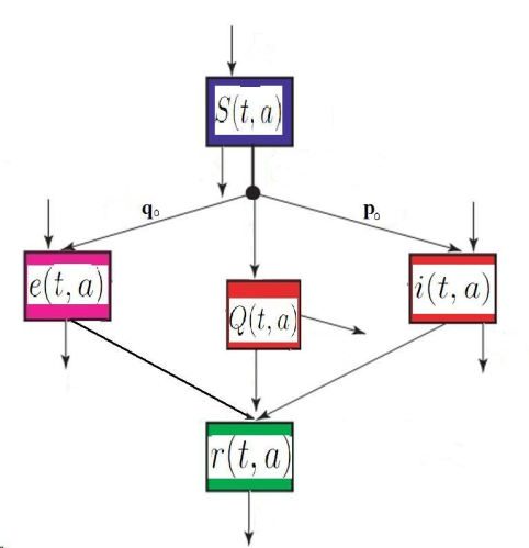
2. Formulation of the Model with Test/Detection, Containment Stage (Identification of Cases, Prophylaxis of Their Close Contacts, Promotion of Hygiene Rules and Protective Actions) and Vertical Transmission in a Closed Population

2.1. The age-structured model with horizontal and perinatal control

The model in a closed population includes: (i) vertical and perinatal transmissions (mother-to-child transmission); (ii) horizontal transmission amongst the whole population [4]. $S(t,a)$, $i(t,a)$, $e(t,a)$ and $r(t,a)$ denotes respectively the densities of susceptible individuals, two different states of infectious individuals and retired/removed individuals. In addition $p_0\in L_{+}^{\infty }(0,\infty )$ is a given function such that $0\le p_0\left(a\right)\le 1$$a.e.$ while $q_0\left(a\right)\equiv 1-p_0\left(a\right)=:\epsilon \left(a\right)p_0\left(a\right)$. Function $q_0$ represents the age-specific probability to enter in state e when becoming infected at age a. Function $p_0$ denotes the probability to develop state i of infection when getting the infection at age a. We refer for application to Nokes et al. [3] for more explanation on the age-dependence susceptibility to the infection in the case of hepatitis B virus (HBV). According to Nokes et al. in [3] function $q_0$ takes the form $q_0\left(a\right)=\kappa e^{-r{a}^s}$ for some suitable (positive) parameter set for $(\kappa ,r,s)$. In order to take into account this age-specific susceptibility dependence, Ducrot et al. [7] consider the simplest prototypical shape curve of the form

$$q_0\left(a\right)=\kappa e^{-ra}$$

(1)

for some $\kappa \in [0,1]$ and $r>0$. This differential susceptibility is a very important aspect of HBV infection: according to CDC (Centers for Disease Control and Prevention, USA: www.cdc.gov.) about 90% of children will remain chronically infected with HBV while 95% of adults will develop acute infection and will completely recover from HBV infection. We consider an age-dependent test/detection and cure/containment rate $\Psi (t,a)$ (with $0\le \Psi (t,a)\le 1$ for a.e. t and a) in our age-structured model: we will use it to partially control the evolution of the disease in horizontal transmission, while vertical transmission will be controlled through birth(s) coming from infectious individuals with a term $v\left(t\right)$ (with $0\le v\left(t\right)\le 1$) where $t\in [0;T)$ and $a\in [0;A)$ lower than fixed values $A\in (0;+\infty )$ and $T\in (0;+\infty )$ respectively seen as (maximal) lifespan and horizon time. $0\le \delta \le 1$ is the reduction in risk due to prior exposure to containment stage (identification of cases , prophylaxis of their close contacts, promotion of hygiene rules and protective actions). That means: $\delta =0$ corresponds to a perfect detection/containment and $\delta =1$ corresponds to a totally imperfect strategy of medical test/detection and containment/quarantine. $\mu \left(a\right)\ge 0$ denotes the natural death rate. ${\mu }_I\left(a\right)\ge 0$ and ${\mu }_E\left(a\right)\ge 0$ are respectively the additional death rates for $i-$state and $e-$state. ${ϵ}_x$ is the retired rate from the $x-$state, $x\in \left\{i,e\right\}$. The term $\lambda \left(t,a\right)$ corresponds to the age-specific force of infection and follows the usual law of mass-action, that reads as

$$\lambda (t,a)={\int }_0^{\infty }{\beta }_i(a,a^{\prime })i(t,a^{\prime })d{a}^{\prime }+{\int }_0^{\infty }{\beta }_e(a,a^{\prime })e(t,a^{\prime })d{a}^{\prime }$$

Here, ${\beta }_i(a,a^{\prime })$ and ${\beta }_e(a,a^{\prime })$ denote the (finite essential supremum and compact supported) contact transmission rates between acute infected individuals (i) or chronic carriers (e) of chronological age $a^{\prime }$ with susceptible of chronological age a respectively.

Remark 1. In fact we can consider $a\in (0,\infty )$ instead of $a\in (0,A)$. All the supports of the coefficients (seen as functions of a) are included in $(0,A)$. We set a compartment Q of contained individuals (isolated and spreading no more the disease) and neglect births coming from this compartment.

In this section we will consider the following (chronological “a”) age-structured model with a test/containment strategy Ψ and vertical transmission

$$\begin{array}{cc}& \left({\partial }_t+{\partial }_a+\mu \left(a\right)\right)S(t,a)=-\lambda (t,a)\left[1-\left(1-\delta \right)\Psi (t,a)\right]S(t,a),\hfill \\ & \left({\partial }_t+{\partial }_a+\left({\mu }_I\left(a\right)+\mu \left(a\right)+{ϵ}_i\left(a\right)\right)\right)i(t,a)=\lambda (t,a)p_0\left(a\right)\left[1-\left(1-\delta \right)\Psi (t,a)\right]S(t,a),\hfill \\ & \left({\partial }_t+{\partial }_a+\left({\mu }_E\left(a\right)+\mu \left(a\right)+{ϵ}_e\left(a\right)\right)\right)e(t,a)=\lambda (t,a)q_0\left(a\right)\left[1-\left(1-\delta \right)\Psi (t,a)\right]S(t,a),\hfill \\ & \left({\partial }_t+{\partial }_a+\mu \left(a\right)+ϵ\left(a\right)\right)Q(t,a)=\lambda (t,a)\left(1-\delta \right)\Psi (t,a)S(t,a)-\pi \left(a\right)Q(t,a)\hfill \\ & \left({\partial }_t+{\partial }_a+\mu \left(a\right)\right)r(t,a)={ϵ}_{i_1}\left(a\right)i(t,a)+{ϵ}_{e_1}\left(a\right)e(t,a)+\pi \left(a\right)Q(t,a)\hfill \end{array}$$

(2)

with $0\le {ϵ}_{i_1}\le {ϵ}_i$ and $0\le {ϵ}_{e_1}\le {ϵ}_e$. Moreover ${\partial }_x\equiv \frac{\partial }{{\partial }_x}$.

This problem is supplemented together with the boundary conditions (for $t\in [0;T)$):

$$\begin{array}{cc}\hfill S(t,0)& ={\int }_0^{\infty }f\left(a\right)\left[S(t,a)+b_1\left(a\right)i(t,a)+b_2\left(a\right)e(t,a)+b_3\left(a\right)r(t,a)\right]da\hfill \\ \hfill i(t,0)& ={\int }_0^{\infty }f\left(a\right)v\left(t\right)c_1\left(a\right)p(t,a)\left[(1-b_1\left(a\right))i(t,a)+(1-b_2\left(a\right))e(t,a)\right]da\hfill \\ \hfill e(t,0)& ={\int }_0^{\infty }f\left(a\right)v\left(t\right)(1-c_1\left(a\right))\epsilon \left(a\right)p(t,a)\left[(1-b_1\left(a\right))i(t,a)+(1-b_2\left(a\right))e(t,a)\right]da\hfill \\ \hfill Q(t,0)& =0\hfill \\ \hfill r(t,0)& =0\hfill \end{array}$$

and initial data (for $a\in [0;A)$): $S(0,a)=S_0\left(a\right)$, $i(0,a)=i_0\left(a\right)$, $e(0,a)=e_0\left(a\right)$, $r(0,a)=r_0\left(a\right)$, $Q(0,a)=Q_0\left(a\right)$. f is similar to the fertility function. $p(t,a)$ will be explicitly described in subsection 3.3. Moreover functions $v,c_1,b_1,b_2$ and $b_3$ are $[0;1]$-valued. We assume here that infected offspring come from “mixing” between infectives. It is also assumed in some diseases transmitted by genes.

We voluntary choose to skip compartment of latent individuals since its dynamic is relatively fast (around 3 months as average time for hepatitis B). The first assumption here is to consider retired few such as $b_3=0$ a.e. Then we will note that the r component of the system is decoupled from the other components and has therefore no impact upon the long term behaviour of the system (2).

2.2. About the Well-posedness of the Age-Structured Model

It is possible to prove (in brief) that (2) is well-posed using semigroup theory [8] in suitable Banach or Sobolev spaces (or refer to a general context in Brokate [9]) as follows.

The system (2) can be re-written under the form of a Cauchy problem:

$$\left\{\begin{array}{c}\frac{dw\left(t\right)}{dt}=Aw\left(t\right)+F(t,w\left(t\right)):=G(t,w\left(t\right))\\ w\left(0\right)=w_0\in D\left(A\right)\end{array}\right.$$

(3)

with

$$w\left(t\right)\equiv \left(\begin{array}{c}0\\ 0\\ 0\\ 0\\ 0\\ S(t,.)\\ i(t,.)\\ e(t,.)\\ r(t,.)\\ Q(t,.)\end{array}\right)$$

and

$$D\left(A\right)={\left\{0\right\}}^5\times {\left(W^{11}(0;+\infty )\right)}^5$$

Let $v\equiv \left(\begin{array}{c}{\alpha }_1\\ {\alpha }_2\\ {\alpha }_3\\ {\alpha }_4\\ {\alpha }_5\\ \widehat{S}\\ \widehat{i}\\ \widehat{e}\\ \widehat{r}\\ \widehat{Q}\end{array}\right)$ in the Banach space

$$X={\mathbb{R}}^5\times {\left(L^1(0;+\infty )\right)}^5$$

endowed with the usual norm

$${∥v∥}_X={\Sigma }_{i=1}^{i=5}\left|{\alpha }_i\right|+{\int }_0^{\infty }\left[\left|\widehat{S}\left(a\right)\right|+\left|\widehat{i}\left(a\right)\right|+\left|\widehat{e}\left(a\right)\right|+\left|\widehat{r}\left(a\right)\right|+\left|\widehat{Q}\left(a\right)\right|\right]da$$

The natural positive cone of X is

$$X_{+}={[0;+\infty )}^5\times {\left(L_{+}^1(0;+\infty )\right)}^5$$

We also define

$$X_0={\left\{0\right\}}^5\times {\left(L^1(0;+\infty )\right)}^5$$

and its positive cone

$$X_{0+}={\left\{0\right\}}^5\times {\left(L_{+}^1(0;+\infty )\right)}^5$$

We set $u\equiv \left(\begin{array}{c}0\\ 0\\ 0\\ 0\\ 0\\ \widehat{S}\\ \widehat{i}\\ \widehat{e}\\ \widehat{r}\\ \widehat{Q}\end{array}\right)$ and the linear and closed operator defined on $D\left(A\right)$ by:

$$\begin{array}{cccc}A:& D\left(A\right)& \to & X\\ & u& ⟼& \left(\begin{array}{c}\widehat{S}\left(0\right)\\ \widehat{i}\left(0\right)\\ \widehat{e}\left(0\right)\\ \widehat{r}\left(0\right)\\ \widehat{Q}\left(0\right)\\ -\frac{d\widehat{S}}{da}-\left(\Psi (.)+\mu (.)\right)\widehat{S}\\ -\frac{d\widehat{i}}{da}-\left({\mu }_I(.)+\mu (.)\right)+{ϵ}_i(.)\widehat{i}\\ -\frac{d\widehat{e}}{da}-\left({\mu }_E(.)+\mu (.)+{ϵ}_e(.)\right)\widehat{e}\\ -\frac{d\widehat{r}}{da}-\mu (.)\widehat{r}+{ϵ}_{i_1}(.)\widehat{i}+{ϵ}_{e_1}(.)\widehat{e}+\pi (.)\widehat{Q}\\ -\frac{d\widehat{Q}}{da}-\left(\mu (.)+ϵ(.)+\pi (.)\right)\widehat{Q}\end{array}\right)\end{array}$$

It always exists $\overline{\mu }\in [0;+\infty )$ such that: $\forall a\ge 0,\mu \left(a\right)\ge \overline{\mu }$. Then we have for each $\lambda >-\overline{\mu }$

$${(\lambda -A)}^{-1}{X}_{+}\subset X_{0+}$$

(4)

and $(-\overline{\mu },\infty )\subset \rho \left(A\right)$ with

$${\parallel (\lambda -A)}^{-1}{\parallel }_{ℒ\left(X\right)}\le \frac{1}{\lambda +\overline{\mu }},\forall \lambda >-\overline{\mu }$$

(5)

The part $A_0$ of A defined by

$$\begin{array}{cccc}{A}_0:& D\left(A_0\right)& \to & X\\ & u& ⟼& \left(\begin{array}{c}0\\ 0\\ 0\\ 0\\ 0\\ -\frac{d\widehat{S}}{da}-\left(\Psi (.)+\mu (.)\right)\widehat{S}\\ -\frac{d\widehat{i}}{da}-\left({\mu }_I(.)+\mu (.)+{ϵ}_i(.)\right)\widehat{i}\\ -\frac{d\widehat{e}}{da}-\left({\mu }_E(.)+\mu (.)+{ϵ}_e(.)\right)\widehat{e}\\ -\frac{d\widehat{r}}{da}-\mu (.)\widehat{r}+{ϵ}_{i_1}\left(a\right)\widehat{i}+{ϵ}_{e_1}(.)\widehat{e}+\pi (.)\widehat{Q}\\ -\frac{d\widehat{Q}}{da}-\left(\mu (.)+ϵ(.)+\pi (.)\right)\widehat{Q}\end{array}\right)\end{array}$$

with $D\left(A_0\right)$ defined by

$$\left\{u\equiv \left(\begin{array}{c}0\\ 0\\ 0\\ 0\\ 0\\ \widehat{S}\\ \widehat{i}\\ \widehat{e}\\ \widehat{r}\\ \widehat{Q}\end{array}\right)\in D\left(A\right):Au\in \overline{D\left(A\right)},\widehat{S}\left(0\right)=\widehat{i}\left(0\right)=\widehat{e}\left(0\right)=\widehat{r}\left(0\right)=\widehat{Q}\left(0\right)=0\right\}$$

$A_0$ verifies the Hille-Yosida property: It exists $\overline{\mu }\in [0;+\infty )$ such that $\forall a\ge 0,\mu \left(a\right)\ge \overline{\mu }$ and we have for each $\lambda >-\overline{\mu }$

$$\parallel {(\lambda -A_0)}^{-1}{\parallel }_{\mathcal{L}\left(X_0\right)}\le \frac{1}{\lambda +\overline{\mu }},\forall \lambda >-\overline{\mu }$$

(6)

and (by lemma 2.1 of [10, Ducrot et al. 2010]): $X_1:=\overline{D\left(A_0\right)}$. Assumption 2.2 of [10, Ducrot et al. 2010, pp. 267] is satisfied. Then its lemma 2.3 [10, Ducrot et al. 2010, pp. 267] applies: $A_0$ is the infinitesimal generator of a $C_0$-semigroup ${\left(T_{A_0}\left(t\right)\right)}_{t\ge 0}$ on $X_1$.

We define the Fréchet differentiable in the second variable u ( and then “locally” Lipschitz in u) perturbation (for each $t\ge 0$):

$$\begin{array}{cccc}F(t,.):& X_0& \to & X\\ & u& ⟼& F(t,u(.\left)\right)\end{array}$$

with

$$F(t,u(.))=\left(\begin{array}{c}-{\int }_0^{\infty }f\left(a\right)\left[\widehat{S}\left(a\right)+b_1\left(a\right)\widehat{i}\left(a\right)+b_2\left(a\right)\widehat{e}+b_3\left(a\right)\widehat{r}\left(a\right)\right]da\\ -{\int }_0^{\infty }f\left(a\right)v\left(t\right)c_1\left(a\right)p(t,a)\left[(1-b_1\left(a\right))\widehat{i}\left(a\right)+(1-b_2\left(a\right))\widehat{e}\left(a\right)\right]da\\ -{\int }_0^{\infty }f\left(a\right)v\left(t\right)(1-c_1\left(a\right))\epsilon \left(a\right)p(t,a)\left[(1-b_1\left(a\right))\widehat{i}\left(a\right)+(1-b_2\left(a\right))\widehat{e}\left(a\right)\right]da\\ 0\\ 0\\ -{\lambda }^{*}(.)\left[1-\left(1-\delta \right)\Psi (t,.)\right]\widehat{S}\\ {\lambda }^{*}(.)p_0(.)\left[1-\left(1-\delta \right)\Psi (t,.)\right]\widehat{S}\\ {\lambda }^{*}(.)q_0(.)\left[1-\left(1-\delta \right)\Psi (t,.)\right]\widehat{S}\\ 0\\ {\lambda }^{*}(.)\left(1-\delta \right)\Psi (t,.)\widehat{S}\end{array}\right)$$

with

$${\lambda }^{*}\left(a\right)={\int }_0^{\infty }{\beta }_i(a,a^{\prime })\widehat{i}\left(a^{\prime }\right)d{a}^{\prime }+{\int }_0^{\infty }{\beta }_e(a,a^{\prime })\widehat{e}\left(a^{\prime }\right)d{a}^{\prime }$$

The model (3) is well posed as it admits an integrated solution w defined on a maximal time interval $[0;T]$ (eventually $T\to +\infty$ through a bounded dissipativity property) [10,11]. w satisfies (in Bochner sense for integrals):

$${\int }_0^{t}w\left(s\right)ds\in D\left(A\right)$$

and

$$w\left(t\right)=w_0+A{\int }_0^{t}w\left(s\right)ds+{\int }_0^{t}F(s,w\left(s\right))ds\text{(}t\ge 0\text{)}$$

In the sequel we denotes by ${\nu }_i\left(a\right):=\left({\mu }_I\left(a\right)+\mu \left(a\right)+{ϵ}_i\left(a\right)\right)$ and ${\nu }_e\left(a\right):=\left({\mu }_I\left(a\right)+\mu \left(a\right)+{ϵ}_e\left(a\right)\right)$ the global mortalities for i and e compartments respectively. Moreover ϵ is the additional mortality for the Q-compartment.

Remark 2. It is possible to add a transition at constant proportional rate from $i–$state to $e–$state in diseases like hepatitis B [3].

3. Optimal Control Problem

Let $D=\left[0;T\right]\times \left[0;A\right]$. We want to find an optimal strategy Ψ such that we minimize the functional

$$\overline{C}(T,A,\Psi ,v)={\int }_0^T{\int }_0^{A}L(t,a,y(t,a),\Psi (t,a),v\left(t\right))dadt$$

such that (see useful definition in next subsection or [5], pp. 48)

$$L(t,a,y(t,a),\Psi (t,a),v\left(t\right))=d\left(a\right)y(t,a)+c\left(\Psi (t,a)\right)+z\left(v\left(t\right)\right)$$

(with real valued functions c and z) on the admissible set for $\left(\Psi ,v\right)$:

$$E^{ad}=\left\{\left(n,m\right)\in L^{\infty }\left(D:\mathbb{R}\right)\times L^{\infty }\left(\left[0;T\right]:\mathbb{R}\right)\left|n\left(x\right),m\left(y\right)\in [0;1]\right.\text{for}\text{a.e.}(x,y)\in D\times [0;T]\right\}$$

Here $d\left(a\right)\in {\mathbb{R}}^2$ (in row) is the damage caused by a member of age a, while the second and third terms in L represent the cost of the control due to detection/test, cure and fight against perinatal or mother to child transmission.

3.1. About Existence of Optimal Control $(\widehat{\Psi },\widehat{v})$

In this work, we assume the existence of a minimum $\left(\widehat{y},\widehat{p},\widehat{q},\widehat{\Psi },\widehat{v}\right)$. However, an interesting work by Picart et al. [12] could be used (in with section 2 of [12]) to prove the existence of at least one optimum. Similarly to [12], positivity of the biological system (2) implies that the total number of newborns cannot be larger than the total number of newborns without admissible positive control ($v=1$ and $\Psi =1$). Using then the lower bound d of the continuous cost function $C_{T,A}(\Psi ,v):=\overline{C}(T,A,\Psi ,v)$ and the point dissipative semiflow of the dynamical system (2) one can prove the existence of a bounded minimizing sequence ${({\Psi }_k,v_k)}_{k\in \mathbb{N}}$ of $E^{ad}$ converging up to a subsequence to an admissible control. Finally, the sequence ${\left\{C_{T,A}({\Psi }_k,v_k)\right\}}_{k\in \mathbb{N}}$ converges as $k\to +\infty$ to d, the well-posedness of the minimization problem [W]: “ $mi{n}_{\Psi ,v}\overline{C}(T,A,\Psi ,v)$ in the admissible set $E^{ad}$ ” in the sense where [W] admits at least one optimum. About these control $(\Psi ,v)$, the convexity with respect to control $(v,\Psi )$ of the integrand of the $C_{T,A}(\Psi ,v)$ (for existence) and a sufficiently small time-interval (for uniqueness) could also be helpful. This work focuses on determination of candidates to optimal control for optimal solution of the cost functional.

3.2. Context of a Result of Feichtinger et al. [5]

We apply then Theorem 1, ([5], pp. 57) with necessary optimality conditions (Pontryagin’s maximum principle) ([5], pp. 56) using the following notations, assumptions and short results focusing on $\left(\widehat{y},\widehat{p},\widehat{q},\widehat{\Psi },\widehat{v}\right)$:

• $U=V=[0;1]$$\subset \mathbb{R}$ (in this epidemiological case);
• $y\equiv \left(\begin{array}{c}i\\ e\end{array}\right):D\to {\mathbb{R}}^2$, $p:D\to \mathbb{R};$
• $q:\left[0;T\right]\to {\mathbb{R}}^2$, $\Psi :D\to U$, $v:\left[0;T\right]\to V;$
• $L:D\times {\mathbb{R}}^2\times \mathbb{R}\times {\mathbb{R}}^2\times U\times V\to \mathbb{R}$, $f:D\times {\mathbb{R}}^2\times \mathbb{R}\times {\mathbb{R}}^2\times U\to {\mathbb{R}}^2;$
• $g:D\times \left[0;A\right]\times {\mathbb{R}}^2\times U\to \mathbb{R}$, $h:D\times {\mathbb{R}}^2\times \mathbb{R}\times {\mathbb{R}}^2\times U\to {\mathbb{R}}^2;$
• $y_0\equiv \left(\begin{array}{c}{i}_0\\ e_0\end{array}\right):\left[0;A\right]\to {\mathbb{R}}^2$, $\phi :\left[0;T\right]\times {\mathbb{R}}^2\times V\to {\mathbb{R}}^2;$
• Admissible control is any couple $\left(\Psi ,v\right)$ of measurable functions

  $$\Psi :D\to U\mathbf{and}v:D\to V$$
• The function $L,f,g,h,y_0,\phi$ are Carathéodory (that is, measurable in the (eventually) three variables $t,a,a^{\prime }$ and continuous in the rest of variables), locally essentially bounded, differentiable in $\left(y,p,q,v\right),$ with locally Lipschitz partial derivatives, uniformly with respect to $\Psi \in U$ and $\left(t,a\right)\in D$, $a^{\prime }\in \left[0;A\right]$;
• Moreover using result of Sell and You [13], we can prove that there is a compact $Z\subset {\mathbb{R}}^6$ such that for every admissible control $(\Psi ,v)$ the system has a unique solution $\left(S,y,p,q\right)$ on D in the sense of ([5], pp. 51) and the solutions takes values in Z.
• We assume that there exists an optimal solution $\left(\widehat{y},\widehat{p},\widehat{q},\widehat{\Psi },\widehat{v}\right)$ (see interesting results of M. Brokate [9]);
• (see [5], pp. 56) $f(t,a):=f(t,a,\widehat{y}(t,a),\widehat{p},\widehat{q},\widehat{\Psi })$;
• (see [5], pp. 56) $f(t,a,\Psi ):=f(t,a,\widehat{y}(t,a),\widehat{p},\widehat{q},\Psi )$;
• (see [5], pp. 56) $g(t,a,a^{\prime },\Psi )=g(t,a,a^{\prime },\widehat{y}(t,a),\Psi )$; $h(t,a)=h(t,a,\widehat{y}(t,a),\widehat{p}(t,a),\widehat{q}\left(t\right),\widehat{\Psi })$; $h(t,a,\Psi )=h(t,a,\widehat{y}(t,a),\widehat{p}(t,a),\widehat{q}\left(t\right),\Psi )$;

3.3. Necessary Optimality Conditions for the Model Studied

We define these expressions following our model (2):

• $g(t,a,a^{\prime },y(t,a),\Psi (t,a))=p_0\left(a\right)\left[{\beta }_i(a,a^{\prime })i(t,a^{\prime })+{\beta }_e(a,a^{\prime })e(t,a^{\prime })\right];$
• $p(t,a):={\int }_0^{A}g(t,a,a^{\prime },y(t,a),\Psi (t,a))d{a}^{\prime };$
• $f(t,a,y(t,a),p(t,a),q(t),\Psi (t,a\left)\right)$ is defined by

  $$p(t,a)\left[1-(1-\delta )\Psi (t,a)\right]S(t,a)\left(\begin{array}{c}1\\ \epsilon \left(a\right)\end{array}\right)-\left({\nu }_i\left(a\right),{\nu }_e\left(a\right)\right)y(t,a)$$
• $h(t,a,y(t,a),p(t,a),\widehat{q}(t,a),\widehat{\Psi })\equiv h(t,a,y(t,a),p(t,a))$ is defined by

  $$\left(\begin{array}{c}f\left(a\right)c_1\left(a\right)p(t,a)\left[(1-b_1\left(a\right))i(t,a)+(1-b_2\left(a\right))e(t,a)\right]\\ f\left(a\right)(1-c_1\left(a\right))\epsilon \left(a\right)p(t,a)\left[(1-b_1\left(a\right))i(t,a)+(1-b_2\left(a\right))e(t,a)\right]\end{array}\right)$$
• $q\left(t\right):={\int }_0^{A}h(t,a,y(t,a),p(t,a))da$, $\phi (t,q(t),v(t\left)\right):=v\left(t\right)q\left(t\right)$,
• $y(t,0):=\phi (t,q(t),v(t\left)\right)$
• $G_{ie}\left((r_1,r_2)\right):=\left({\nu }_i\left(a\right)r_1;{\nu }_e\left(a\right)r_2\right)$, $K_{ie}\left(a\right):={\left(1;\epsilon \left(a\right)\right)}^T.$

We introduce (according to [5], pp. 56) the following adjoint system for the adjoint functions $(\xi ,\eta ,\zeta )$, considered as row-vector functions (while y, p and q are column-vectors in $L^{\infty }\left(D:{\mathbb{R}}_{+}^2\right)$, $L^{\infty }\left(D:{\mathbb{R}}_{+}\right)$, $L^{\infty }\left(\left[0;T\right]:{\mathbb{R}}_{+}^2\right)$) from $L^{\infty }\left(D:{\mathbb{R}}^2\right)\times L^{\infty }\left(D:\mathbb{R}\right)\times L^{\infty }\left(\left[0;T\right]:{\mathbb{R}}^2\right)$

$$\begin{array}{cc}\hfill -\left({\partial }_t+{\partial }_a\right)\xi (t,a)& =d\left(a\right)+G_{ie}\left(\xi (t,a)\right)+\zeta \left(t\right)f\left(a\right)p(t,a)(1-b_1\left(a\right))\left(c_1\left(a\right);(1-c_1\left(a\right))\right)\hfill \\ & +{\int }_0^A{p}_0\left(a\right)\eta (t,a^{\prime })\left({\beta }_i(a,a^{\prime });{\beta }_e(a,a^{\prime })\right)d{a}^{\prime }\hfill \\ \hfill \xi (T,a)& =0\hfill \\ \hfill \xi (t,A)& =0\hfill \end{array}$$

with

$$\begin{array}{cc}\hfill \zeta \left(t\right)& =v\left(t\right)\xi (t,0)\hfill \\ \hfill \eta (t,a)& =\left[1-\left(1-\delta \right)\xi (t,a)\right]S(t,a)\xi (t,a)K_{ie}\left(a\right)+f\left(a\right)\zeta (t,a)W\left(y(t,a)\right)\hfill \end{array}$$

where

$$W\left(y(t,a)\right)=\left(\begin{array}{c}{c}_1\left(a\right)\left[(1-b_1\left(a\right))i(t,a)+(1-b_2\left(a\right))e(t,a)\right]\\ (1-c_1\left(a\right))\epsilon \left(a\right)\left[(1-b_1\left(a\right))i(t,a)+(1-b_2\left(a\right))e(t,a)\right]\end{array}\right)$$

For the solution $\left(\widehat{y},\widehat{p},\widehat{q}\right)$, and the corresponding solution $(\xi ,\eta ,\zeta )$ of the adjoint system (existing by Theorem 1 or Proposition 2 [5], pp. 57) we define (as [5]) the boundary and distributed Hamiltonians ([5], pp. 57):

$$\left\{\begin{array}{c}{H}_b(t,v)=\xi (t,0)\phi (t,v)+{\int }_0^{A}L(t,b,v)db\\ H(t,a,\Psi )=L(t,a,\Psi )+\xi (t,a)f(t,a,\Psi )+{\int }_0^A\eta (t,a^{\prime })g(t,a^{\prime },a,\Psi )d{a}^{\prime }+\zeta \left(t\right)h(t,a,\Psi )\end{array}\right.$$

The following proposition relies to the Theorem 1(Pontryagin’s maximum principle [5] with proof on page 64) and straightforward computations.

Proposition 3.

We assume that there exists an optimal control $\left(\widehat{\Psi },\widehat{v}\right)$ and the corresponding solution $\left(\widehat{S},\widehat{y},\widehat{p},\widehat{q},\widehat{\Psi },\widehat{v}\right)$ that minimizes the single-objective cost functional $C_{T,A}(\Psi ,v):=\overline{C}(T,A,\Psi ,v)$ under assumptions in section 3.2 with

$$\left(\widehat{y},\widehat{p},\widehat{q},\widehat{\Psi },\widehat{v}\right)\in L^{\infty }\left(D:{\mathbb{R}}^2\right)\times L^{\infty }\left(D:\mathbb{R}\right)\times L^{\infty }\left(\left[0;T\right]:{\mathbb{R}}^2\right)\times L^{\infty }\left(D:U\right)\times L^{\infty }\left(\left[0;T\right]:V\right).$$

Then

a- 

For a.e $t_0\in \left[0;T\right]$, $a_0\in \left[0;A\right]$ and $(t,a)\in D$

$$\left\{\begin{array}{c}\frac{\partial H_b}{\partial v}(t_0,\widehat{v}\left(t_0\right))\left(v-\widehat{v}\left(t_0\right)\right)\ge 0,\forall v\in V\\ H(t,a,u)-H(t,a,\widehat{\Psi }(t,a))\ge 0,\forall u\in U\end{array}\right.$$

b- 

Moreover the minimization conditions of the Hamiltonian gives:

$$\begin{array}{cc}\hfill c^{\prime }(\Psi (t,a))& =(1-\delta )p(t,a)\widehat{S}(t,a)\xi (t,a)\left(\begin{array}{c}1\\ \epsilon \left(a\right)\end{array}\right)\hfill \\ \hfill z^{\prime }\left(v\left(t\right)\right)& =-\xi (t,0)q\left(t\right)\hfill \end{array}$$

c- 

If $c^{\prime }$ and $z^{\prime }$ are invertible (as for $c\left(s\right)=w_1{s}^2$ and $z\left(s\right)=w_2{s}^2$) then optimal control is explicitly described (for $0\le v\le 1$) by:

$$\left\{\begin{array}{c}\widehat{\Psi }(t,a)=min\left\{1;max\left\{0;{\left[c^{\prime }\right]}^{-1}\left((1-\delta )\widehat{p}(t,a)\widehat{S}(t,a)\widehat{\xi }(t,a)\left(\begin{array}{c}1\\ \epsilon \left(a\right)\end{array}\right)\right)\right\}\right\}\\ \widehat{v}\left(t\right)=min\left\{1;max\left\{0;{\left[z^{\prime }\right]}^{-1}\left(-\widehat{\xi }(t,0)\widehat{q}\left(t\right)\right)\right\}\right\}\end{array}\right.$$

4. Discussion

We know that $c^{\prime }$ and ${\left[c^{\prime }\right]}^{-1}$ have the same variation: then assuming that $c^{\prime }$ is monotonic implies the same variation for ${\left[c^{\prime }\right]}^{-1}$. If $c^{\prime }$ is increasing (as in the particular case $c\left(s\right)=w_1{s}^2$ or generally c is convex), then the optimal effort, $\widehat{\Psi }$, roughly increases $(1-\delta )$ and hence so does the number of those cured by the test/detection and containment stage. It possible to apply this result on 20 years in the case of hepatitis B in a pygmy group named Baka living in the heart of the forest within the east of Cameroon (Africa) with 5647 peoples (data in Foupouapouognigni Y. [4] in 2010). We evaluate [3,7] $p_0$ with least mean squares as $p_0\left(a\right)=1-0.643.e^{-0.156a}$ in a situation of endemicity when the basic reproduction rate is greater than one. It is also possible to choose a linear boundary conditions on i and e such that in subsection 3.3: $g(t,a,a^{\prime },y(t,a),\Psi (t,a))=p_0\left(a\right)\beta (t,a)$ and get interesting results.

References

1. Mclean, A.R.; Blumberg, B.S. Modeling the impact of Mass vaccination against Hepatitis B I. Model formulation and parameter estimation. Proc. Biol. Sci. 1994, 256, 7–15. [Google Scholar] [CrossRef]
2. Sharpe, F.; Lotka, A. A problem in age-distribution. Philos. Mag. 1911, 6, 435–438. [Google Scholar] [CrossRef]
3. Nokes, D.J.; Hall, A.J.; Edmunds, W.J.; Medley, G.F.; Whittle, H.C. The influence of age on the development of the hepatitis B carrier state. Proc. R. Soc. Lond. B Biol. Sci. 1993. [Google Scholar] [CrossRef]
4. Foupouapouognigni, Y.; Sadeuh Mba, S.A.; A Betsem, E.B.; Rousset, D.; Froment, A.; Gessain, A.; Njouom, R. Hepatitis B and C virus infections in the three pygmy groups in Cameroon. J. Clin. Microbiol. 2011, 49, 737–740. [Google Scholar] [CrossRef] [PubMed]
5. Feichtinger, G.; Tragler, G.; Veliov, V.M. Optimality conditions for age-structured control systems. J. Math. Anal. Appl. 2003, 288, 47–68. [Google Scholar] [CrossRef]
6. Sharomi, O.; Malik, T. Optimal control in epidemiology. Ann. Oper. Res. 2015. [Google Scholar] [CrossRef]
7. Ducrot, A.; Houpa, D.D.E.; Kouakep, T.Y. An age-structured model with differential susceptibility: Application to Hepatitis B Virus transmission. Available online: http://arxiv.org/abs/1505.06431 (accessed on 20 May 2015).
8. Inaba, H. Threshold and stability results for an age-structured epidemic model. J. Math. Biol. 1990, 28, 411–434. [Google Scholar] [CrossRef] [PubMed]
9. Brokate, M. Pontryagin’s principle for control problems in age-dependent population dynamics. J. Math. Biol. 1985, 23, 75–101. [Google Scholar] [CrossRef]
10. Ducrot, A.; Magal, P.; Prevost, K. Integrated semigroups and parabolic equations. Part I: Linear perburbation of almost sectorial operators. J. Evol. Equ. 2010, 10, 263–291. [Google Scholar] [CrossRef]
11. Pazy, A. Semigroups of Linear Operators and Applications to Partial Differential Equations; Springer-Verlag: Berlin, Germany, 1983. [Google Scholar]
12. Picart, D.; Ainseba, B.; Milner, F. Optimal control problem on insect pest populations. Applied Mathematics Letter. 2011, 2, 1160–1164. [Google Scholar] [CrossRef]
13. Sell, G.R.; You, Y. Dynamics of Evolutionary Equations; Springer: New York, NY, USA, 2002. [Google Scholar]