Two Dimensional Temperature Distributions in Plate Heat Exchangers: An Analytical Approach

Abstract

Analytical solutions are developed to work out the two-dimensional (2D) temperature changes of flow in the passages of a plate heat exchanger in parallel flow and counter flow arrangements. Two different flow regimes, namely, the plug flow and the turbulent flow are considered. The mathematical formulation of problems coupled at boundary conditions are presented, the solution procedure is then obtained as a special case of the two region Sturm-Liouville problem. The results obtained for two different flow regimes are then compared with experimental results and with each other. The agreement between the analytical and experimental results is an indication of the accuracy of solution method.

1. Introduction

The study of the coupled forms of heat transfer between forced convection flows and conduction in surfaces is very important due to the existence of these simultaneous effects in practical heat transfer processes. In particular, the design and performance of counter flow multilayered heat exchangers offer excellent opportunities to analyze these complex physical phenomena. Many theoretical investigations of heat transfer characteristics of heat exchangers under plug, laminar, and turbulent flows have been published in the literature. Specifically, research on fin efficiency, double pipe, and parallel plate exchangers is progressing. In connection with the conjugate heat transfer process over surfaces, the effect of wall heat conduction and convective heat transfer has been analyzed in several works.

The temperature distribution in a horizontal flat plate of finite thickness was analyzed by Luikov [1] and Payvar [2]. In this conjugate problem the lower surface was maintained at a uniform temperature, while the upper surface was transferring heat to a laminar boundary layer by convection. Two approximate solutions were presented by Luikov [1], based respectively on differential and integral analyses. The first solution was performed considering low Prandtl number assumption, while the second solution was conducted using polynomial forms for the velocity and temperature profiles. In the case of large Prandtl numbers the Lighthill approximation [3] was used by Payvar [2] and an integral equation was obtained and then solved numerically.

From the practical point of view, the specific wall temperature boundary condition is the least important, since its use as a representation of an actual condition in a plate heat exchanger is applicable only for certain special limiting cases. Boundary conditions that specify heat fluxes apply more directly to any actual situation, such as coolant passages of nuclear reactors.

Except for certain special circumstances, none of the boundary conditions treated in the literature would be applicable. In view of the practical importance of heat exchangers in general, it is surprising that investigations of applicable Sturm-Liouville problem have not been investigated. A possible reason for this appears to be related to the applicability of the classical mathematical techniques to obtain analytical solutions to similar problems. However, the analytical treatment of Graetz and conjugated Graetz problems is mainly based on the Eigen-function expansion technique in terms of power series in many studies [4]. Nunge and Gill [5] developed an orthogonal expansion technique for solving a new class of counter-flow heat transfer problems. Nunge and Gill [5] solved the exchanger problem assuming fully developed laminar velocity profiles, negligible conduction in the fluid streams, and temperature independent fluid properties.

The main purpose of this paper is conducting an introductory analytical investigation of temperature distribution in parallel flow and counter flow plate heat exchangers using Sturm-Liouville problem. Mehrabian [6] derived one dimensional temperature distributions in plate heat exchangers using four simplifying assumptions. These assumptions were uniform heat flux, constant overall heat transfer coefficient, linear relationship between the overall heat transfer coefficient and cold flow temperature, linear relationship between the overall heat transfer coefficient and temperature difference between cold and hot flows. Ansari et al. [7] developed a mathematical model to analyze the heat transfer characteristics in a double pipe heat exchanger. They used laminar flow assumption for flow in the internal tube and turbulent flow in the annular channel in parallel flow arrangement. The heat transfer coefficients derived for inner flow and outer flow were predicted using the mathematical model and compared with standard correlations. The model deviation from the standard correlation was less than 10 percent [7]. This paper is an extension of [6,7], using analytical approach to obtain temperature distributions in plate heat exchangers in longitudinal direction as well as in the direction perpendicular to the plates.

The temperature distribution in plate heat exchangers is obtained based on a two region Sturm-Liouville system consisting of two equations coupled at common boundary. The solutions of this system form an infinite sequence of Eigen functions with corresponding eigenvalues. If the velocity distributions are assumed to be uniform, the Eigen functions are the familiar tabulated functions and eigenvalues are given by the positive nonzero roots of an eigenvalue transcendental equation. The plug flow and the turbulent flow models of the heat exchanger fluid flows are utilized in this paper with the following idealizations:

1-

At the inlet to each channel the temperature is uniform in the channel cross-section.

2-

Frictional heating is negligible.

3-

Longitudinal heat conduction in the plates is negligible.

4-

Physical properties are temperature independent.

5-

Longitudinal heat conduction in the fluids is negligible.

6-

The effect of corrugations in flow and heat transfer is neglected.

The first three idealizations are reasonable in most heat exchangers applications. The fourth idealization is normally acceptable when considering density, specific heat and thermal conductivity for liquid-liquid applications. The variations of viscosity with respect to temperature in plate heat exchanger channels were studied by Mehrabian et al. [8]. Their study shows, in a plate heat exchanger with water as the process and service fluid the performance does not considerably change when an average viscosity based on T = (T_inlet + T_outlet)/2 is used for each fluid. The accuracy of this assumption is more pronounced when T_in − T_out is not very large.

The fifth idealization has been shown to be valid for a variety of special cases when Peclet numbers are larger than 50 [9,10,11], it seems reasonable to assume that this idealization is valid for the particular cases of interest here, where Peclet number exceeds 50. The sixth idealization can be more realistic by considering the developed plate area instead of the projected plate area in heat transfer calculations.

Figure 1. Plate heat exchanger geometry.

Figure 1. Plate heat exchanger geometry.

2. Problem Description and Mathematical Formulation Based on Plug Flow Model

The plate heat exchanger consists of channels separated by common walls with fluids flowing through the channels, as illustrated in Figure 1. Plate heat exchangers are widely used, their great advantage being their diversity of application and simplicity of construction. They consist of a number of rectangular plates separated with gaskets to contain a constant space and then clamped together. The gaskets control the inlet and outlet ports in the corners of the plates, allowing the hot and cold fluids to flow in alternative channels of the exchanger. Since it is easy to alter the number of plates used in an exchanger, and since a wide variety of flow arrangements is possible, these exchangers can be used for many applications [6].

Based on the previous simplifications, the energy conservation and Fourier’s heat conduction law, for the heat exchanger channels shown in Figure 1 are as follows:

$$u_1\frac{\partial T_1}{\partial z}={\mathsf{\alpha }}_1\frac{{\partial }^2{T}_1}{\partial {x_1}^2}$$

(1)

$${(-1)}^m{u}_2\frac{\partial T_2}{\partial z}={\mathsf{\alpha }}_2\frac{{\partial }^2{T}_2}{\partial {x_2}^2}$$

(2)

where $\mathsf{\alpha }=\frac{k}{\mathsf{\rho }c}$, m = 0 for parallel flow, m = 1 for counter flow, u₁ and u₂ are the absolute values of velocity. The symmetry and wall boundary conditions are:

$$x_i=0: \frac{\partial T_i}{\partial x_i}=0$$

(3)

$$\begin{array}{ccccc}{x}_i=a_i: q_1-q_2=0& & \Rightarrow & & k_1\frac{\partial T_1}{\partial x_1}+k_2\frac{\partial T_2}{\partial x_2}=0\end{array}$$

(4)

Heat balance equation at the interface of fluid 1 and wall (x₁ = a₁) can be expressed as;

$$\begin{array}{ccccc}{q}_1=q_w& & \Rightarrow & & k_1\frac{\partial T_1}{\partial x_1}=k_w\frac{T_2(a_2,z)-T_1(a_1,z)}{b}\end{array}$$

(5)

Equations (1) and (2) are special cases of the two-region Sturm-Liouville problem.

2.1. Dimensionless Equations

The dimensionless space variables for channel 1 and 2 are respectively defined as follows:

$$X_1=\frac{x_1}{a_1}$$

(6)

$$X_2=\frac{x_2}{a_2}$$

(7)

The dimensionless length Z is defined for channels 1 and 2, referenced arbitrarily to the properties of channel 1:

$$Z=\frac{4}{P{e}_1}(\frac{z}{2a_1})$$

(8)

where Pe₁ is the Peclet number for channel 1, defined as:

$$P{e}_1=\frac{2a_1{u}_1}{{\mathsf{\alpha }}_1}$$

(9)

Other dimensionless parameters are defined as follows:

$$H=\frac{c_2{\dot{M}}_2}{c_1{\dot{M}}_1}$$

(10)

$$K=\frac{k_1{a}_2}{k_2{a}_1}$$

(11)

$$K_w=\frac{k_{1}b}{k_w{a}_1}=\frac{\frac{k_1}{a_1}}{\frac{k_w}{b}}=\frac{R_1^{-1}}{R_w^{-1}}=\frac{R_w}{R_1}$$

(12)

$${\mathsf{\psi }}^2=KH$$

(13)

$${\mathsf{\theta }}_i(X_i,Z)=\frac{T_i-T_{c(Z=0)}}{T_{h(Z=0)}-T_{c(Z=0)}}$$

(14)

The governing equations and boundary condition are re-written in terms of dimensionless variables θ_i, X_i and Z:

$$\frac{{\partial }^2{\mathsf{\theta }}_1}{\partial {X_1}^2}=\frac{\partial {\mathsf{\theta }}_1}{\partial Z}$$

(15)

$$\frac{{\partial }^2{\mathsf{\theta }}_2}{\partial {X_2}^2}={(-1)}^m{\mathsf{\psi }}^2\frac{\partial {\mathsf{\theta }}_2}{\partial Z}$$

(16)

$${\mathsf{\theta }}_1(X_1,0)=0$$

(17)

$${\mathsf{\theta }}_2(X_2,0)=1$$

(18)

$$X_i=0: \frac{\partial {\mathsf{\theta }}_i}{\partial X_i}=0$$

(19)

$$X_i=1: K\frac{\partial {\mathsf{\theta }}_1}{\partial X_1}+\frac{\partial {\mathsf{\theta }}_2}{\partial X_2}=0$$

(20)

$$X_i=1:K_W\frac{\partial {\mathsf{\theta }}_1}{\partial X_1}+\mathsf{\theta }(1,Z)_1-{\mathsf{\theta }}_2(1,Z)=0$$

(21)

2.2. Solution

To solve the problem, the method of separation of variables is used. A separation in the following form is assumed for channel 1:

θ₁(X₁,Z) = N₁(Z).M₁(X₁)

(22)

Applying Equation (22) to Equation (15) gives:

$$\frac{M_1^{″}(X_1)}{M_1(X_1)}=\frac{N_1^{\prime }(Z)}{N_1(Z)}=k=-{\mathsf{\lambda }}_n^2$$

(23)

where λ is the Eigen value. Equation (22) will become indeterminate for positive k while for negative k, θ₁ will converge to a limiting value, this is explained with more details in [4,5,12]. The solution for N₁(Z) with respect to λ is:

$$N_1(Z)=e^{-{\mathsf{\lambda }}_n^{2}Z}$$

(24)

Thus

$${\mathsf{\theta }}_1(X_1,Z)={\displaystyle \sum _{n=0}^{\infty }}{C}_n{M}_{1n}(X_1)e^{-{{\mathsf{\lambda }}_n}^2.Z}$$

(25)

A similar method applied to Equation (17) gives:

$${\mathsf{\theta }}_2(X_2,Z)={\displaystyle \sum _{n=0}^{\infty }}{C}_n{M}_{2n}(X_2)e^{-{{\mathsf{\lambda }}_n}^2.Z}$$

(26)

Applying the new variables θ₁ and θ₂ into Equation (15) and Equation (16) yields:

$$M_{1n}^{″}(X_1)+{{\mathsf{\lambda }}_n}^2{M}_{1n}(X_1)=0$$

(27)

$$M_{2n}^{″}(X_2)+{(-1)}^m.{\mathsf{\psi }}^{2.}{{\mathsf{\lambda }}_n}^2{M}_{2n}(X_2)=0$$

(28)

Applying the new variables θ₁ and θ₂ into Equation (20) to Equation (22) gives:

$$M_{1n}^{\prime }(0)=0$$

(29)

$$M_{2n}^{\prime }(0)=0$$

(30)

$$K.M_{1n}^{\prime }(1)+M_{2n}^{\prime }(1)=0$$

(31)

$$K_W.M_{1n}^{\prime }(1)+M_{1n}(1)-M_{2n}(1)=0$$

(32)

2.3. Eigenvalue Equation

Assuming M_1n(X₁) = A.F (λ, X₁) and M_2n(X₂) = B.G (λ, X₂), where A and B are arbitrary constants, for λ = λ₀, λ₁, λ₂, λ₃, ..., Equation (31) and Equation (32) respectively become:

$$KA{F}_{X_1}^{\prime }(\mathsf{\lambda },1)+B{G}_{X_2}^{\prime }(\mathsf{\lambda },1)=0$$

(33)

$$A[K_W{F}_{X_1}^{\prime }(\mathsf{\lambda },1)+F(\mathsf{\lambda },1)]-BG(\mathsf{\lambda },1)=0$$

(34)

We can write Equations (33) and (34) as:

$$\left[\begin{array}{ccc}{\text{KF}}_{{\mathrm{x}}_1}^{\prime }(\mathsf{\lambda },1)\hfill & & \hfill {\mathrm{G}}_{{\mathrm{x}}_2}^{\prime }(\mathsf{\lambda },1)\\ K_W{F}_{X_1}^{\prime }(\mathsf{\lambda },1)+F(\mathsf{\lambda },1)\hfill & & \hfill - G(\mathsf{\lambda },1)\end{array}\right]\left[\begin{array}{c}A\\ B\end{array}\right]=\left[\begin{array}{c}0\\ 0\end{array}\right]$$

In order this system of simultaneous homogeneous linear algebraic equations have nonzero solutions for A and B, the coefficient determinant must be made equal to zero by proper choice of λ:

$$\left|\left[\begin{array}{ccc}{\text{KF}}_{{\mathrm{x}}_1}^{\prime }(\mathsf{\lambda },1)\hfill & & \hfill {\mathrm{G}}_{{\mathrm{x}}_2}^{\prime }(\mathsf{\lambda },1)\\ K_W{F}_{X_1}^{\prime }(\mathsf{\lambda },1)+F(\mathsf{\lambda },1)\hfill & & \hfill - G(\mathsf{\lambda },1)\end{array}\right]\right|=0$$

This gives the eigenvalue equation:

$$F(\mathsf{\lambda },1)G_{X_2}^{\prime }(\mathsf{\lambda },1)+K{F}_{X_1}^{\prime }(\mathsf{\lambda },1)G(\mathsf{\lambda },1)+K_W{F}_{X_1}^{\prime }(\mathsf{\lambda },1)G_{X_2}^{\prime }(\mathsf{\lambda },1)=0$$

(35)

In order to find λ = λ₀, λ₁, λ₂, λ₃, ... for each condition (K, Kw, H), Equation (35) should be solved. S(λ) represents Equation (35) for parallel flow and counter flow conditions in Table 1.

Table 1. F, G and Eigen functions for parallel flow and counter flow plate heat exchangers.

Type	F(λ, X1)	G(λ, X2)	S(λ)
Parallel flow	cos(λX1)	cos(ψλX2)	$\begin{array}{l}\text{cos}(\mathsf{\lambda })\text{sin}(\mathsf{\psi }\mathsf{\lambda })+\frac{K}{\mathsf{\psi }}\text{sin}(\mathsf{\lambda })\text{cos}(\mathsf{\psi }\mathsf{\lambda })-K_W\mathsf{\lambda }\\ \text{sin}(\mathsf{\lambda })\text{sin}(\mathsf{\psi }\mathsf{\lambda })=0\end{array}$
Counter flow	cos(λX1)	cosh(ψλX2)	$\begin{array}{l}\text{cos}(\mathsf{\lambda })\sinh (\mathsf{\psi }\mathsf{\lambda })-\frac{K}{\mathsf{\psi }}\text{sin}(\mathsf{\lambda })\text{cosh}(\mathsf{\psi }\mathsf{\lambda })-K_W\mathsf{\lambda }\\ \text{sin}(\mathsf{\lambda })\sinh (\mathsf{\psi }\mathsf{\lambda })=0\end{array}$

Table 1. F, G and Eigen functions for parallel flow and counter flow plate heat exchangers.

Type	F(λ, X1)	G(λ, X2)	S(λ)
Parallel flow	cos(λX1)	cos(ψλX2)	$\begin{array}{l}\text{cos}(\mathsf{\lambda })\text{sin}(\mathsf{\psi }\mathsf{\lambda })+\frac{K}{\mathsf{\psi }}\text{sin}(\mathsf{\lambda })\text{cos}(\mathsf{\psi }\mathsf{\lambda })-K_W\mathsf{\lambda }\\ \text{sin}(\mathsf{\lambda })\text{sin}(\mathsf{\psi }\mathsf{\lambda })=0\end{array}$
Counter flow	cos(λX1)	cosh(ψλX2)	$\begin{array}{l}\text{cos}(\mathsf{\lambda })\sinh (\mathsf{\psi }\mathsf{\lambda })-\frac{K}{\mathsf{\psi }}\text{sin}(\mathsf{\lambda })\text{cosh}(\mathsf{\psi }\mathsf{\lambda })-K_W\mathsf{\lambda }\\ \text{sin}(\mathsf{\lambda })\sinh (\mathsf{\psi }\mathsf{\lambda })=0\end{array}$

For K = 1, H = 1, Kw = 0 we have following Eigenvalues (parallel flow condition):

λ = λ₀, λ₁, λ₂, λ₃, λ₄, λ₅…

λ = 1.5705, 3.1415, 4.7125, 6.2835, 7.8535, 9.4245…

and for K = 1, H = 1, Kw = 0 we have following Eigenvalues (Counter flow condition):

λ = λ₀, λ₁, λ₂, λ₃, λ₄, λ₅…

λ = 3.9266, 7.0686, 10.2102, 13.3518, 16.4934, 19.6350…

Equation (33) gives:

$$B=-K\frac{F_{X_1}^{\prime }(\mathsf{\lambda },1)}{G_{X_2}^{\prime }(\mathsf{\lambda },1)}A$$

(36)

Since the system is homogeneous, either A or B can be chosen arbitrarily, Hence:

$$A=G_{X_2}(\mathsf{\lambda },1)$$

(37)

The Eigen functions M_1n and M_2n can be represented by:

$$M_{1n}(X_1)=AF(\mathsf{\lambda },X_1)=G_{X_2}(\mathsf{\lambda },1)F(\mathsf{\lambda },X_1)$$

(38)

$$M_{2n}(X_2)=BG(\mathsf{\lambda },X_2)=-K{F}_{X_1}(\mathsf{\lambda },1)G(\mathsf{\lambda },X_2)$$

(39)

Constants A and B calculated in this section satisfy Equation (34). Ansari [13] proved that for arbitrary constants ψ, K, Kw, and values of A, and B obtained in this section Equation (34) is true. He [13] also calculated the values of λ for which the boundary conditions are fulfilled.

2.4. Finding F(λ, X₁) and G(λ, X₂)

The solution for Equation (27) along with boundary condition, Equation (20) is:

$$M_{1n}(X_1)=AF(\mathsf{\lambda },X_1)=A\text{cos}(\mathsf{\lambda }{X}_1)$$

(40)

Equation (28) and boundary condition for channel 2 are:

$$M_{2n}^{″}(X_2)+{(-1)}^m{\mathsf{\psi }}^2{\mathsf{\lambda }}^2{M}_{2n}(X_2)=0$$

(41)

$$M_{2n}^{\prime }(0)=0$$

(42)

The solution for counter flow arrangement (m = 1) is:

$$M_{2n}(X_2)=BG(\mathsf{\lambda },X_2)=B\text{cosh}(\mathsf{\psi }\mathsf{\lambda }{X}_2)$$

(43)

F(λ, X₁), G(λ, X₂) and Eigen functions are given in Table 1 for plate heat exchangers. M_1n(X₁) and M_2n(X₂) are also given in Equations (38) and (39).

2.5. Orthogonality of the Eigen functions

The orthogonality condition for the M_1n and M_2n will now be established. The differential Equation (27) is first manipulated for n = i and j in the same manner used to derive properties of the familiar Sturm-liouville system. For example, Equation (27) is written for n = i and then for n = j with i ≠ j. the equation for n = i is multiplied by M_1j and the equation for n = j is multiplied by M_1i. The two resulting equations are subtracted, simplified and then integrated between X₁ = 0 and X₁ = 1. The following equation is obtained:

$$\left({\mathsf{\lambda }}_j^2-{\mathsf{\lambda }}_i^2\right){\displaystyle \underset{0}{\overset{1}{\int }}}{M}_{1j}(X_1)M_{1i}(X_1)d{X}_1=M_{1j}(1)M_{1i}^{\prime }(1)-M_{1i}(1)M_{1j}^{\prime }(1)$$

(44)

In a similar manner, Equation (28) is written for n = i and then for n = j with i ≠ j. the equation for n = i is multiplied by M_2j and the equation for n = j is multiplied by M_2i. The two resulting equations are subtracted, simplified and then integrated between X₂ = 0 and X₂ = 1. The following equation is obtained;

$${\mathsf{\psi }}^2\left({\mathsf{\lambda }}_j^2-{\mathsf{\lambda }}_i^2\right){\displaystyle \underset{0}{\overset{1}{\int }}}{M}_{2j}(X_2)M_{2i}(X_2)d{X}_2=M_{2j}(1)M_{2i}^{\prime }(1)-M_{2i}(1)M_{2j}^{\prime }(1)$$

(45)

Equations (44) and (45) can be related to each other using the coupling boundary conditions at X = 1. Thus, Equations (31) and (32) respectively become:

$$M_{2n}^{\prime }(1)=-K{M}_{1n}^{\prime }(1)$$

(46)

$$M_{2n}(1)=M_{1n}(1)+K_w{M}_{1n}^{\prime }(1)$$

(47)

Using these conditions in Equations (44) and (45) gives:

$${\displaystyle \underset{0}{\overset{1}{\int }}}{M}_{1i}(X_1)M_{1j}(X_1)d{X}_1+{\displaystyle \underset{0}{\overset{1}{\int }}}H{M}_{2j}(X_2)M_{2i}(X_2)d{X}_2=0 i\ne j$$

(48)

Equation (48) is the orthogonality condition for the Eigen function M_1n and M_2n. For the case of i = j = n, Equation (48) leads to a normalizing factor defined by:

$$N_n={\displaystyle \underset{0}{\overset{1}{\int }}}{M}_{1n}^2(X_1)d{X}_1+{\displaystyle \underset{0}{\overset{1}{\int }}}H{M}_{2n}^2(X_2)d{X}_2$$

(49)

Equations (38) and (39) for the case of n = 0 with λ = 0 give

M₁₀ = M₂₀ = 1

Applying the above condition into Equation (49) gives:

$$N_0=1+H$$

(50)

2.6. Finding C_n and θ_i

The following expansions are considered regarding Equations (25) and (26) at Z = 0:

$$0={\displaystyle \sum _{n=0}^{\infty }}{C}_n{M}_{1n}(X_1)$$

(51)

$$1={\displaystyle \sum _{n=0}^{\infty }}{C}_n{M}_{2n}(X_2)$$

(52)

Multiplying Equation (51) by M_1n(X₁)dX₁ and Equation (52) by H.M_2n(X₂)dX₂, adding the resulting expressions and integrating between X_i = 0 and X_i = 1 using Equation (49), the following equation for the C_n is obtained:

$$C_n=\frac{1}{N_n}{\displaystyle \underset{0}{\overset{1}{\int }}}H.M_{2n}(X_2)d{X}_2$$

(53)

Equations (50) and (53) give:

$$C_0=\frac{H}{N_n}=\frac{H}{1+H}$$

(54)

Using Equations (38), (39) and (53) and simplifying the results gives:

$$A_{1n}=C_n.M_{1n}(X_1)=\frac{2G_{X2}(\mathsf{\lambda },1)F(\mathsf{\lambda },X_1)}{\mathsf{\psi }{\mathsf{\lambda }}^2{S}^{\prime }(\mathsf{\lambda })}$$

(55)

$$A_{2n}=C_n.M_{2n}(X_2)={(-1)}^{1-m}.\frac{2.K.F_{X_1}(\mathsf{\lambda },1).G(\mathsf{\lambda },X_2)}{\mathsf{\psi }.{\mathsf{\lambda }}^2.S^{\prime }(\mathsf{\lambda })}$$

(56)

where S′(λ) is the differential of the Eigen function. The solution for the two-dimensional temperature distribution can subsequently be written as:

$${\mathsf{\theta }}_i(X_i,Z)=\frac{H}{1+H}+{\displaystyle \sum _{n=1}^{\infty }}{A}_{in}(X_i).e^{-{\mathsf{\lambda }}_n^2.Z}$$

(57)

The average temperature can be used as one-dimensional form of temperature distribution:

$${\mathsf{\theta }}_{Bi}(X_i)={\displaystyle \underset{0}{\overset{1}{\int }}}{\mathsf{\theta }}_i(Xi,Z)d{X}_i=\frac{H}{1+H}+{\displaystyle \underset{0}{\overset{1}{\int }}}\left({\displaystyle \sum _{n=1}^{\infty }}{A}_{in}(X_i).e^{-{\mathsf{\lambda }}_n.Z}\right)d{X}_i$$

(58)

3. Modification for the Turbulent Flow

Equations (1) and (2) used for plug flow condition in Section 2 can be applied for turbulent flow when α is replaced by α + ε [14]. Since α = k/ρc, the general form for Equations (1) and (2) applied to turbulent flow becomes:

$$\frac{\partial }{\partial X}\left[\left(k+c\mathsf{\rho }\mathsf{\epsilon }\right)\frac{\partial T}{\partial X}\right]=c\mathsf{\rho }u\frac{\partial T}{\partial Z}$$

(59)

In this equation ε represents a turbulent diffusivity for heat transfer. The term k + cρε can be interpreted as an effective total conductivity, k_t written as:

$$k_t=k\left(1+\frac{\mathsf{\epsilon }}{v}\text{Pr}\right)$$

(60)

where v is the kinematic viscosity and Pr is the Prandtl number. Now an average effective conductivity k_m is defined:

$$k_m={\displaystyle \underset{0}{\overset{1}{\int }}}{k}_{t}dX$$

(61)

The k_m value for the parallel plate channel was obtained experimentally by Lyon [15], He proposed the following correlation for predicting k_m with respect to Peclet number:

$$k_m=\frac{k}{6}\left(5.8+0.02P{e}^{0.8}\right)$$

(62)

The average effective conductivity, k_m, must be applied to Equations (11) and (12) in order to convert the plug flow solution into the turbulent flow solution. In other words, K in Equation (11) and K_W in Equation (12) are respectively replaced by:

$$K_t=\left(\frac{k_{m1}{a}_2}{k_{m2}{a}_1}\right)$$

(63)

and

$$K_{Wt}=\left(\frac{k_{m1}b}{k_w{a}_1}\right)$$

(64)

4. Results

The results are presented in four different cases representing in Figure 2, Figure 3, Figure 4 and Figure 5.

Figure 2. Temperature distribution for a parallel flow plate heat exchanger (Plug flow). (a) Two dimensional temperature distribution for K = 1, H = 0.5, K_W = 0; (b) Two dimensional temperature distribution for K = 1, H = 1, K_W = 0; (c) Two dimensional temperature distribution for K = 1, H = 2, K_W = 0.

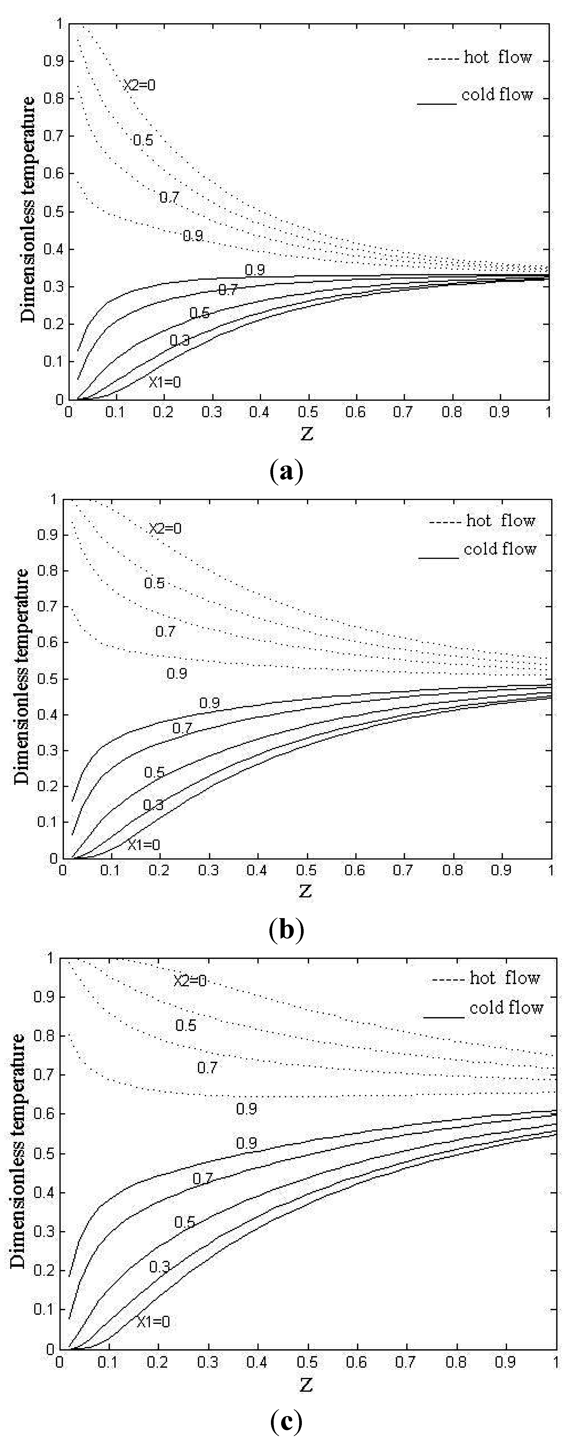
Figure 2. Temperature distribution for a parallel flow plate heat exchanger (Plug flow). (a) Two dimensional temperature distribution for K = 1, H = 0.5, K_W = 0; (b) Two dimensional temperature distribution for K = 1, H = 1, K_W = 0; (c) Two dimensional temperature distribution for K = 1, H = 2, K_W = 0.

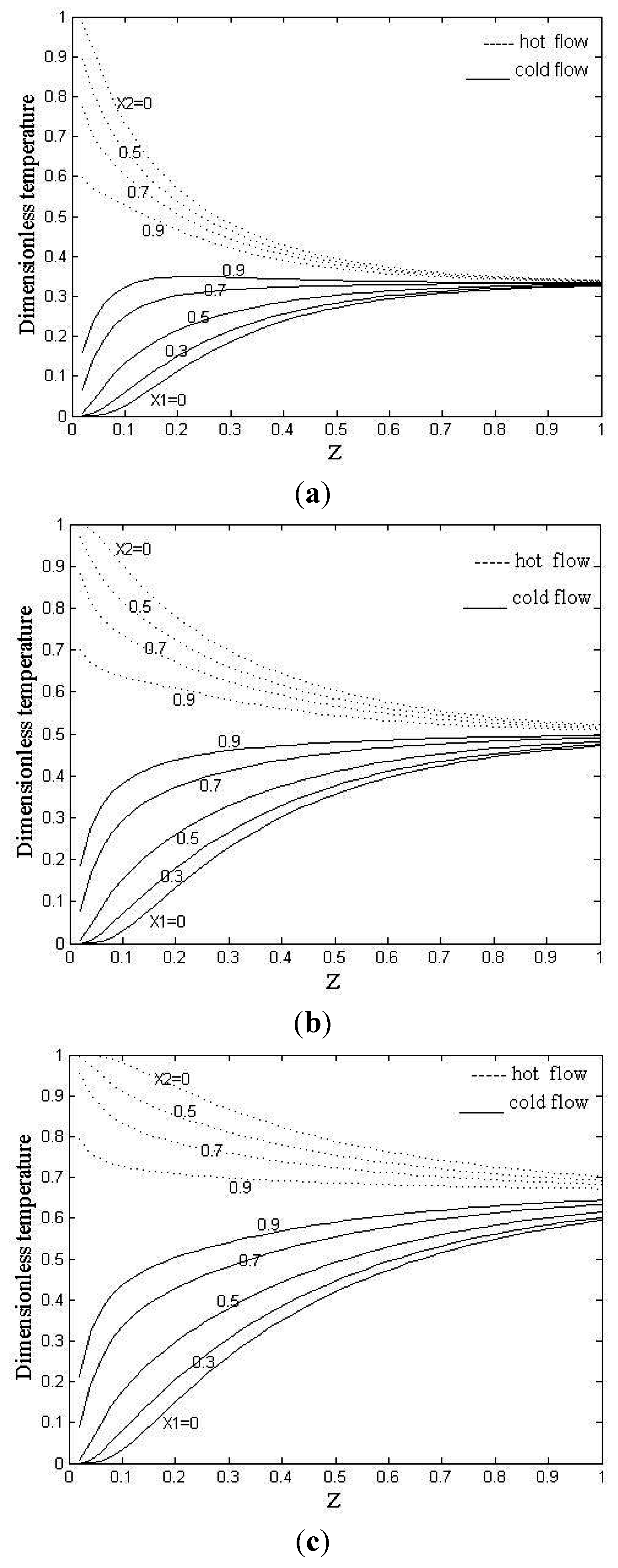
Figure 3. Temperature distribution for a parallel flow plate heat exchanger (Turbulent flow). (a) Two dimensional temperature distribution for K = 1, H = 0.5, K_W = 0, and K_t = 0.33; (b) Two dimensional temperature distribution for K = 1, H = 1, K_W = 0 and K_t = 0.33; (c) Two dimensional temperature distribution for K = 1, H = 2, K_W = 0 and K_t = 0.33.

Figure 3. Temperature distribution for a parallel flow plate heat exchanger (Turbulent flow). (a) Two dimensional temperature distribution for K = 1, H = 0.5, K_W = 0, and K_t = 0.33; (b) Two dimensional temperature distribution for K = 1, H = 1, K_W = 0 and K_t = 0.33; (c) Two dimensional temperature distribution for K = 1, H = 2, K_W = 0 and K_t = 0.33.

Figure 4. Temperature distribution for a counter flow plate heat exchanger (Plug flow). (a) Two dimensional temperature distribution for K = 1, H = 0.5, K_W = 0; (b) Two dimensional temperature distribution for K = 1, H = 1, K_W = 0; (c) Two dimensional temperature distribution for K = 1, H = 2, K_W = 0.

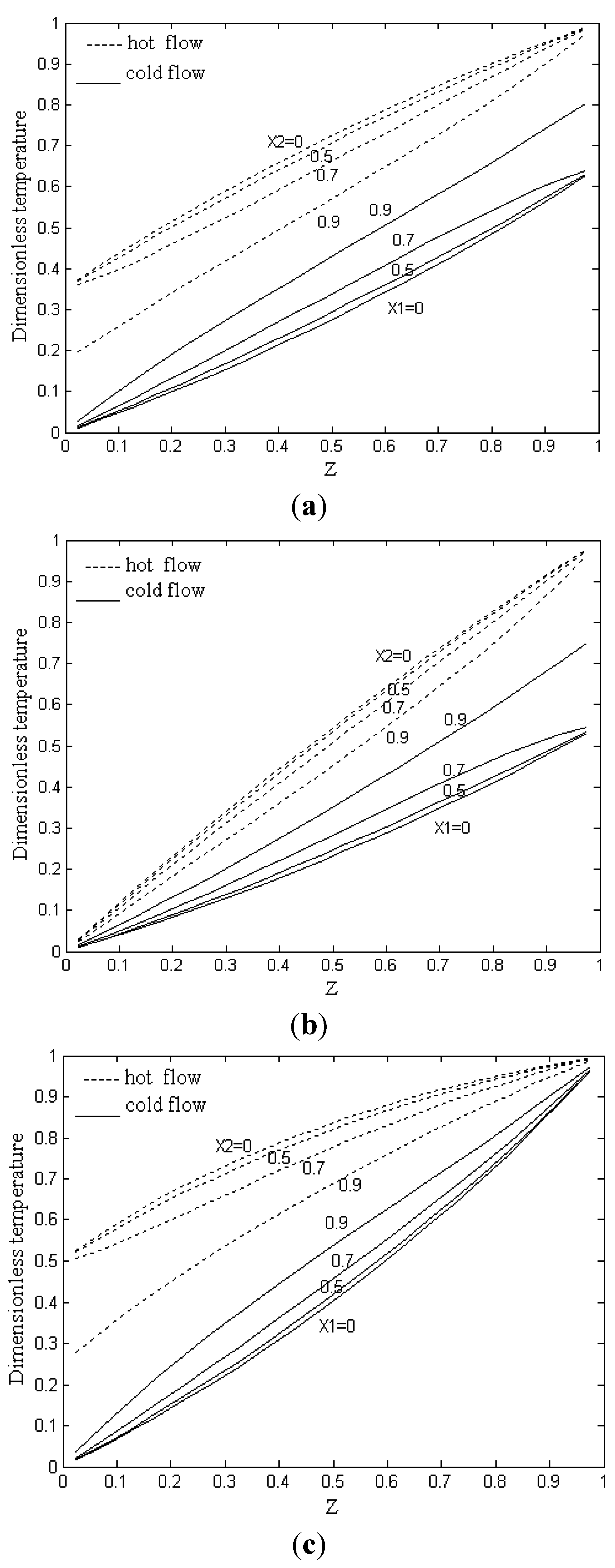
Figure 4. Temperature distribution for a counter flow plate heat exchanger (Plug flow). (a) Two dimensional temperature distribution for K = 1, H = 0.5, K_W = 0; (b) Two dimensional temperature distribution for K = 1, H = 1, K_W = 0; (c) Two dimensional temperature distribution for K = 1, H = 2, K_W = 0.

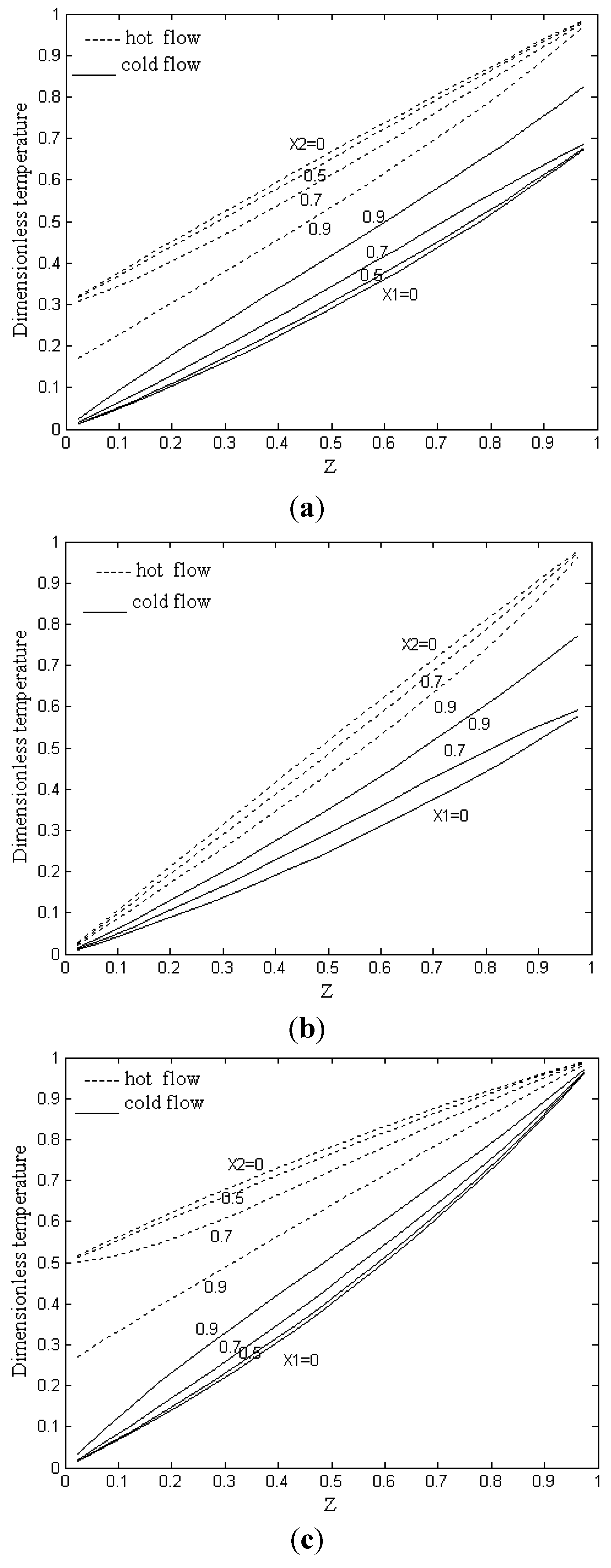
Figure 5. Temperature distribution for a counter flow plate heat exchanger (Turbulent flow). (a) Two dimensional temperature distribution for K = 1, H = 0.5, K_W = 0 and K_t = 0.33; (b) Two dimensional temperature distribution for K = 1, H = 1, K_W = 0, and K_t = 0.33; (c) Two dimensional temperature distribution for K = 1, H = 2, K_W = 0 and K_t = 0.33.

Figure 5. Temperature distribution for a counter flow plate heat exchanger (Turbulent flow). (a) Two dimensional temperature distribution for K = 1, H = 0.5, K_W = 0 and K_t = 0.33; (b) Two dimensional temperature distribution for K = 1, H = 1, K_W = 0, and K_t = 0.33; (c) Two dimensional temperature distribution for K = 1, H = 2, K_W = 0 and K_t = 0.33.

4.1. Parallel Flow Arrangement-Plug Flow Regime (Pe₁ = 75000, and Pe₂ = 3500)

The dimensionless temperature distributions for hot and cold flows in this case are shown in Figure 2 for K_w = 0, where K_w is defined in Equation (12), the wall thermal resistance (R_w) is much smaller than the fluid thermal resistance (R_w << R₁), therefore K_W is very small (K_W ≈ 0).

4.2. Parallel Flow Arrangement-Turbulent Flow Regime (Pe₁ = 75000, and Pe₂ = 3500)

The dimensionless temperature distributions for hot and cold flows in this case are shown in Figure 3 for K_w = 0 and K_t = 0.33.

4.3. Counter Flow Arrangement-Plug Flow Regime (Pe₁ = 75000, and Pe₂ = 3500)

The dimensionless temperature distributions for hot and cold flows in this case are shown in Figure 4 for K_w = 0.

4.4. Counter Flow Arrangement-Turbulent Flow Regime (Pe₁ = 75000, and Pe₂ = 3500)

The dimensionless temperature distributions for hot and cold flows in this case are shown in Figure 5 for K_w = 0 and K_t = 0.33.

5. Comparison, Validation, and Discussion

The temperature distribution obtained for counter flow arrangement is compared with the established experimental data available in the literature using similar plate dimensions and flow details [6,16,17]. To get a clearer picture of the problem, a plate heat exchanger consisting of four standard plates is considered. Plate dimensions and flow details are shown in Table 2. Fluid temperatures at five intermediate points in the main chevron region are evaluated.

Table 2. Plate dimensions and flow details.

Developed Plate Length	L	1 m
Flow wide	W	0.35 m
Flow thickness	2a1, a2	0.00367 m
Wall thickness	b	0.0006 m
Thermal conductivity of wall	kw	73 W/m.K
	Hot fluid	Cold fluid
Inlet temperature	77.9 °C	47.9 °C
Outlet temperature	71.7 °C	76.9 °C
Heat capacity	4191J/kg.K	4184 J/kg.K
Mass flow rate	472.6 kg/h	101.2 kg/h
density	994 kg/m3	994 kg/m3
Kinematics Viscosity × 106	0.461 m2/s	0.623 m2/s
Thermal conductivity	0.664 W/m.K	0.651 W/m.K
Pr	3.48	3.75
Re	406.8	64.4

Table 2. Plate dimensions and flow details.

Developed Plate Length	L	1 m
Flow wide	W	0.35 m
Flow thickness	2a1, a2	0.00367 m
Wall thickness	b	0.0006 m
Thermal conductivity of wall	kw	73 W/m.K
	Hot fluid	Cold fluid
Inlet temperature	77.9 °C	47.9 °C
Outlet temperature	71.7 °C	76.9 °C
Heat capacity	4191J/kg.K	4184 J/kg.K
Mass flow rate	472.6 kg/h	101.2 kg/h
density	994 kg/m3	994 kg/m3
Kinematics Viscosity × 106	0.461 m2/s	0.623 m2/s
Thermal conductivity	0.664 W/m.K	0.651 W/m.K
Pr	3.48	3.75
Re	406.8	64.4

The plate dimensions briefly mentioned in Table 2 correspond to standard APV SR3 chevron plates, which are widely used in the process industry [16]. The flow details given in Table 2 have been applied in a test machine. The local temperatures along the central exchanger channel (cold fluid flow) have been measured experimentally [16].

The dimensionless parameters for analytical procedure are as follows:

H = 4.68, K_t = 1.03, K_t,w = 0.0015, ψ² = 4.59

(65)

The experimental data [15] and analytical-numerical results developed in [6] are listed in Table 3. In reality, the temperature varies not only along z, but also along x. Table 3 is dedicated to the variations of temperature along z.

Table 3. Temperature distribution of the cold flow in two sides of the central channel of the plate heat exchanger.

TE (°C)	TN (°C)	Error	T (°C)	Error	Distance
47.9	47.9	0	47.9	0	0 m
61.9	60.3	2.6	62.6	3.1	1/6 m
66.8	67.6	1.2	66.1	0.4	2/6 m
70.2	72	2.6	69.7	1.5	3/6 m
72.6	74.5	2.6	72.1	2	4/6 m
74.3	76	2.2	74.6	1.8	5/6 m
76.9	76.9	0	76.9	0	1 m

T_E: Experimental data [14], T_N: Local temperature of plate heat exchanger using the analytical-numerical method developed in [15] for constant overall heat transfer coefficient, T: Local temperature of plate heat exchanger using the analytical method developed in this paper.

Table 3. Temperature distribution of the cold flow in two sides of the central channel of the plate heat exchanger.

TE (°C)	TN (°C)	Error	T (°C)	Error	Distance
47.9	47.9	0	47.9	0	0 m
61.9	60.3	2.6	62.6	3.1	1/6 m
66.8	67.6	1.2	66.1	0.4	2/6 m
70.2	72	2.6	69.7	1.5	3/6 m
72.6	74.5	2.6	72.1	2	4/6 m
74.3	76	2.2	74.6	1.8	5/6 m
76.9	76.9	0	76.9	0	1 m

T_E: Experimental data [14], T_N: Local temperature of plate heat exchanger using the analytical-numerical method developed in [15] for constant overall heat transfer coefficient, T: Local temperature of plate heat exchanger using the analytical method developed in this paper.

Mehrabian et al. [17] established an experimental technique to measure the local temperatures along the flow channels of a plate heat exchanger. Mehrabian, et al. [18] also conducted a three dimensional computational analysis to investigate the hydrodynamics and thermal characteristics of plate heat exchangers. In this investigation they predicted the temperature, pressure, and velocity distributions in the flow channels of a plate heat exchanger. The present paper tackles the same problem from an analytical point of view, and therefore completes this cycle of computational, experimental, and analytical methodologies. Each methodology has its own difficulties, analytical approach however requires the governing equations are as simplified as possible and this leads to certain simplifying assumptions. The major assumptions affecting the analytical results are:

• Ignoring the heat transfer enhancement in the development region for the fluids,
• Not taking account of the effect of corrugations by assuming the plates are flat, and
• Assuming turbulent flow in the flow channels while the Reynolds numbers are not large enough. It should be mentioned that the flow visualization experiments [19] support this assumption.

6. Conclusions

In this study, the mathematical model of the heat transfer phenomena in a plate heat exchanger with counter flow or parallel flow arrangements has been developed and investigated. The analytical solution is obtained based on a two region Sturm-Liouville system consisting of two equations coupled at a common boundary. In order to provide mathematical simplicity, a plug flow model of the heat exchanging fluids were utilized for this analysis. An approximate method was developed for converting the plug flow formulation into the turbulent flow formulation. The mathematical method performed in this study can be applied for the prediction of the temperature distribution. The predictions of the method developed in this study are in close agreement with experimental results available in the literature.