Numerical Solution of Multiterm Fractional Differential Equations Using the Matrix Mittag–Leffler Functions

Abstract

Multiterm fractional differential equations (MTFDEs) nowadays represent a widely used tool to model many important processes, particularly for multirate systems. Their numerical solution is then a compelling subject that deserves great attention, not least because of the difficulties to apply general purpose methods for fractional differential equations (FDEs) to this case. In this paper, we first transform the MTFDEs into equivalent systems of FDEs, as done by Diethelm and Ford; in this way, the solution can be expressed in terms of Mittag–Leffler (ML) functions evaluated at matrix arguments. We then propose to compute it by resorting to the matrix approach proposed by Garrappa and Popolizio. Several numerical tests are presented that clearly show that this matrix approach is very accurate and fast, also in comparison with other numerical methods.

1. Introduction

The use of fractional order derivatives is nowadays widespread in many fields. Indeed, the possibility to use any real order improves the modeling of several phenomena in physics, engineering and many application areas. The available literature on fractional calculus is very rich, and we cite only, among the others, [1,2,3,4,5]. It is a fact that the theoretical analysis of fractional differential equations (FDEs) is much more advanced than finding their numerical solution. This topic is indeed very delicate and much more difficult than finding the numerical solution of differential equations of integer order (ODEs). The introduction of effective numerical methods is recent (see, e.g., [6,7,8,9,10,11,12,13] and the books [4,14] together with the references therein). Several numerical methods for FDEs are generalizations of well-established methods for ODEs with appropriate changes. A common problem when dealing with FDEs is the loss of order with respect to the ODE case. This is mainly due to the fact that solutions of FDEs (and their fractional derivatives) are usually not smooth.

In this paper, we address the numerical solution of multiterm fractional differential equations (MTFDEs), that is, FDEs in which multiple fractional derivatives are involved. These turn out to be very helpful in many fields, particularly to model complex multirate physical processes. However, even if many numerical methods for FDEs can be extended to MTFDEs, delicate issues such as numerical stability, convergence or accuracy cannot be easily predicted in this case. Many authors have worked thoroughly on their numerical solution [15,16,17,18,19,20,21,22]. We restrict our attention to the linear case that includes important models, such as the Bagley–Torvik equation [23], the fractional oscillation equation [24] and many others.

Crucial contributions to the numerical solution of MTFDEs came from Diethelm and coauthors [4,16,17,25]. An important result therein is the equivalence between a MTFDE and a single-order system of FDEs [16]. In this paper, we propose a numerical approach that is grounded on this equivalent formulation; indeed, its solution can be expressed in terms of the Mittag–Leffler (ML) function evaluated in the coefficient matrix. The ML function is fundamental in the analysis of fractional calculus, not least because the exact solution of many FDEs can be expressed in terms of this function. However, for a long time, this has been considered only as a theoretical tool because of the lack of effective methods to numerically approximate this function. Only recently have many advances been made for the numerical evaluation of the scalar ML function [26,27,28,29]; the case of matrix arguments has since been analyzed [30,31], and finally a numerical algorithm has been accomplished, which reaches very high accuracies [32]. In this paper, we show the effectiveness of the matrix approach when solving MTFDEs, both in terms of execution time and in terms of accuracy, and also in comparison with some well-established numerical methods. The test equations we consider are well known in literature, and their exact solution is at our disposal. This is fundamental to test the reliability. However, the tests we present show an excellent accuracy, and thus the approach can be favorably applied to solve more general multiterm FDEs.

In particular, among the available numerical methods for MTFDEs, we consider the product integration (PI) rules. These nowadays represent a valuable numerical method for FDEs, although they were originally proposed for the numerical solution of Volterra integral formulas (see, e.g., [33]). Indeed, as a result of the possibility of rewriting any linear FDE as a weakly singular Volterra integral equation of second-type, a generalization of PI rules has been applied to FDEs [12,19,21,34,35,36]. In our numerical tests, we compare the approach we propose to the results given by methods belonging to this class.

The paper is organized as follows: In Section 2, we briefly review the main definitions of fractional calculus, and we linger on the multiterm case. We present the main theoretical tool, given by Diethelm and Ford [16,25], to transform the MTFDE into an equivalent system of FDEs. In Section 3, we address the numerical solution of this equivalent system. This essentially grounds on ML functions with matrix arguments, and we introduce the numerical method proposed by Garrappa and Popolizio [32] to compute matrix ML functions. The performance is tested in Section 4, where we give a comparison with PI methods for several tests; in the same section, a brief description of these methods is presented.

2. Fractional Differential Equations

Fractional derivatives can be introduced by means of the Riemann–Liouville (RL) definition or the Caputo definition [3]. These coincide when equipped with homogeneous initial conditions, while in the more general case, important peculiar features separate them. Both of these have been extensively analyzed and are commonly used. However, in the context of the multiterm case we discuss, the definition by Caputo is generally preferred (see the discussion in [16,17,25]). Thus for any $\alpha \in \mathbb{R}$, the fractional derivative $D^{\alpha }$ is defined as

$$D^{\alpha }y\left(t\right)\equiv \frac{1}{\Gamma (m-\alpha )}{\int }_0^t\frac{y^{\left(m\right)}\left(u\right)}{{(t-u)}^{\alpha +1-m}}du$$

with $\Gamma (·)$ denoting Euler’s gamma function and $m=\lceil \alpha \rceil$ being the smallest integer greater than or equal to $\alpha$. The use of this definition allows us to use as initial conditions the values of y and its derivatives of integer order; that is, we augment the differential equation of order $\alpha$ with initial conditions of the form

$$y^{\left(k\right)}\left(0\right)=y_0^{\left(k\right)},k=0,1,\dots ,m-1$$

We are interested in the numerical solution of linear MTFDEs of the form given by the equation

$$\sum _{k=0}^n{a}_k{D}^{{\alpha }_k}y\left(t\right)=f\left(t\right)$$

(1)

with $a_k\in \mathbb{R},a_n\ne 0$ and $0\le {\alpha }_0<\dots <{\alpha }_n$. The associated initial conditions are   

$$y^{\left(j\right)}\left(0\right)=y_0^{\left(j\right)},j=0,1,\dots ,⌈{\alpha }_n⌉-1$$

The MTFDE (Equation (1)) is defined as commensurate if the numbers ${\alpha }_0,\dots ,{\alpha }_n$ are commensurate, that is, if the quotients ${\alpha }_i/{\alpha }_j$ are rational numbers for all $i,j\in \{0,\dots ,n\}$.

One of the main differences is that for MTFDEs, the RL definition would require initial conditions corresponding to each fractional derivative order that appears in the equations, while the Caputo definition merely requires the initial conditions for integer-order derivatives. Moreover, only the Caputo derivative operator has, under suitable hypotheses on continuity, the semigroup property, which is a fundamental tool to treat the multiterm case (see Theorem 1 in the following).

The analytical solution of the problem (Equation (1)) was thoroughly addressed by Gorenflo and Luchko [15], who gave its explicit expression, through ML-type functions, by using operational calculus for the Caputo fractional derivative.

The analysis of commensurate MTFDEs becomes simpler by applying an approach commonly used for ODEs. Indeed, given an ODE of order 2 or above, it can be converted to a system of first-order ODEs. Analogously, we can rewrite a commensurate MTFDE as a single-order system of FDEs, according to well-known theoretical results [16,25]. We report here the main theorem stating this equivalence (as given in [4]).

Theorem 1.

Consider the equation

$$D^{{\alpha }_k}y\left(t\right)=f(t,y\left(t\right),D^{{\alpha }_1}y\left(t\right),D^{{\alpha }_2}y\left(t\right),\dots ,D^{{\alpha }_{k-1}}y\left(t\right))$$

(2)

subject to the initial condition

$$y^{\left(j\right)}\left(0\right)=y_0^{\left(j\right)},j=0,1,\dots ,⌈{\alpha }_k⌉-1$$

where ${\alpha }_k>{\alpha }_{k-1}>\dots >{\alpha }_1>0,{\alpha }_j-{\alpha }_{j-1}\le 1$ for all $j=2,3,\dots ,k$ and $0<{\alpha }_1\le 1$. Assuming that ${\alpha }_j\in \mathbb{Q}$ for all $j=1,2,\dots ,k$, define M to be the least common multiple of the denominators of ${\alpha }_1,{\alpha }_2,\dots ,{\alpha }_k$, and set $\gamma =1/M$ and $N=M{\alpha }_k$. Then this initial value problem is equivalent to the system of equations

$$\begin{array}{cc}\hfill D^{\gamma }{y}_0\left(t\right)& =y_1\left(t\right)\hfill \\ \hfill D^{\gamma }{y}_1\left(t\right)& =y_2\left(t\right)\hfill \\ \hfill ⋮\\ \hfill D^{\gamma }{y}_{N-2}\left(t\right)& =y_{N-1}\left(t\right)\hfill \\ \hfill D^{\gamma }{y}_{N-1}\left(t\right)& =f(t,y_0\left(t\right),y_{{\alpha }_1/\gamma }\left(t\right),\dots ,y_{{\alpha }_{k-1}/\gamma }\left(t\right))\hfill \end{array}$$

(3)

together with the initial conditions

$$y_j\left(0\right)=\left\{\begin{array}{c}{y}_0^{(j/M)}ifj/M\in {\mathbb{N}}_0\hfill \\ 0else\hfill \end{array}\right.$$

in the following sense:

1.

Whenever $Y:={(y_0,\dots ,y_{N-1})}^T$ with $y_0\in C^{⌈{\alpha }_k⌉}[0,b]$ for some $b>0$ is the solution of the system given by Equation (3), the function $y:=y_0$ solves the multiterm initial value problem of Equation (2).

2.

Whenever $y\in C^{⌈{\alpha }_k⌉}[0,b]$ is a solution of the multiterm initial value problem Equation (2), the vector function $Y:={(y_0,\dots ,y_{N-1})}^T:={(y,D^{\gamma }y,D^{2\gamma }y,\dots ,D^{(N-1)\gamma }y)}^T$ solves the multidimensional initial value problem of Equation (3).

The equivalence stated above can in fact also be applied to any multiterm equation. Indeed, Diethelm and Ford [16] showed that when the orders of the fractional derivatives are approximated by commensurate ones, the errors between the solutions of the two systems are comparable to the errors between the orders, to thus ensure the structural stability. In practice, because any real number can be approximated arbitrarily closely by a rational number, any MTFDE can be approximated arbitrarily closely by a commensurate one; this remark allows us to restrict our attention to the commensurate case.

3. Matrix Approach for the Solution of Linear MTFDEs

As a result of Theorem 1, the linear MTFDE (Equation (1)) can be reformulated in terms of a linear system of FDEs of the form

$$D^{\alpha }Y\left(t\right)=AY\left(t\right)+e_{n}f\left(t\right),Y\left(0\right)=Y_0$$

(4)

where $e_n={\left(0,0,\cdots ,0,1\right)}^T\in {\mathbb{R}}^n$, $Y_0$ is composed in a suitable way on the basis of the initial values, and the coefficient matrix $A\in {\mathbb{R}}^{n\times n}$ is the companion matrix:

$$A=\left(\begin{array}{ccccc}0& 1& 0& \cdots & 0\\ 0& 0& 1& \cdots & 0\\ ⋮& ⋮& ⋮& \ddots & ⋮\\ 0& 0& 0& \cdots & 1\\ -\frac{a_0}{a_n}& -\frac{a_1}{a_n}& -\frac{a_2}{a_n}& \cdots & -\frac{a_{n-1}}{a_n}\end{array}\right)$$

Once the solution $Y\left(t\right)$ of Equation (4) has been computed, we keep only its first component, which, as stated in Theorem 1, corresponds to the (scalar) solution of the MTFDE (Equation (1)).

It is well known that the exact solution $Y\left(t\right)$ of Equation (4) is

$$Y\left(t\right)=E_{\alpha ,1}\left(t^{\alpha }A\right)Y_0+{\int }_0^t{(t-\tau )}^{\alpha -1}{E}_{\alpha ,\alpha }\left({(t-\tau )}^{\alpha }A\right)e_{n}f\left(\tau \right)d\tau$$

(5)

with $E_{\alpha ,\beta }$ denoting the ML function that, for complex parameters $\alpha$ and $\beta$, with $\Re \left(\alpha \right)>0$, is defined by means of the series

$$E_{\alpha ,\beta }\left(z\right)=\sum _{j=0}^{\infty }\frac{z^j}{\Gamma (\alpha j+\beta )},z\in \mathbb{C}$$

(6)

$E_{\alpha ,\beta }\left(z\right)$ is clearly a generalization of the exponential function to which it reduces when $\alpha =\beta =1$, as for $j\in \mathbb{N}$, it is $\Gamma (j+1)=j!$.

The solution is even simpler when $f\left(t\right)$ can be expressed in terms of powers (possibly of non-integer order) of t, as no integral is required. Namely, if

$$f\left(t\right)=\sum _{\nu \in \mathcal{G}}{c}_{\nu }{t}^{\nu }$$

with $\mathcal{G}\subset \{\nu \in \mathbb{R},\nu >-1\}$ being an index set and $c_{\nu }$ being some real coefficients, then, as a result of well-known theoretical results (see, e.g., [3]), the true solution can be written as

$$Y\left(t\right)=E_{\alpha ,1}\left(t^{\alpha }A\right)Y_0+\sum _{\nu \in \mathcal{G}}{c}_{\nu }\Gamma (\nu +1)t^{\alpha +\nu }{E}_{\alpha ,\alpha +\nu +1}\left(t^{\alpha }A\right)e_n$$

(7)

Source terms of this kind are common in applications, often resulting from the approximation of given signals. We thus present the numerical solutions of test cases of this form. The more general situation described in Equation (5) requires exactly the same matrix approach we describe, combined with some quadrature methods.

It is decisive that the solution $Y\left(t\right)$ written as Equation (7) essentially relies on t and not on $[0,t]$; instead, any numerical method for FDEs has to work on the whole interval. This is a fundamental difference and a great strength of the matrix approach, particularly when integration is required for large values of t.

The solution as given in Equation (7) essentially requires the computation of the ML function with the matrix argument $t^{\alpha }A$. The numerical computation of matrix functions is an extensively studied topic that has deserved great attention during the last decades (we refer to Higham [37] for a complete treatise and a full list of references). Only recent studies have considered matrix arguments for the ML function (see, e.g., [30,31,32,38,39]). To be precise, even the numerical scalar case has received poor attention, and only recently has Garrappa [29] developed a powerful Matlab routine (ml.m, available on Matlab website) that gives very accurate results for arguments all over the complex plane. Thereafter, an effective numerical procedure for the matrix case has been proposed [32], and we apply this for our computations. Interestingly, the computation of the matrix ML function turns out to be very accurate, practically close to the machine precision. The resulting matrix approach to approximate Equation (7) thus proves to be very accurate and favorable also for its computational costs; indeed, once the matrices $E_{\alpha ,\beta }\left(t^{\alpha }A\right)$ have been computed, only few additional matrix–vector products and vector sums are needed to obtain the solution.

4. Numerical Solution of FDEs

In this section, we present several numerical tests in order to show the effectiveness of the matrix approach discussed in Section 3. Moreover we compare it with PI rules. We briefly recall here the main features of these methods, while we refer to the related references listed in the introduction and to [21] for a complete treatise on their use for the numerical solution of MTFDEs.

4.1. Product Integration Rules

To introduce PI rules, we first need to recall some basics of fractional calculus (we refer to [4] for details). The RL integral is defined as

$$J^{\alpha }y\left(t\right)=\frac{1}{\Gamma \left(\alpha \right)}{\int }_0^t{(t-u)}^{\alpha -1}y\left(u\right)du$$

(8)

We let $T_j[y;0]$ denote the Taylor polynomial of degree j for the function $y\left(t\right)$ centered at the point 0; then the following relation holds [4]:

$$J^{\alpha }{D}_0^{\alpha }y\left(t\right)=y\left(t\right)-T_{m-1}[y;0]\left(t\right)\mathrm{for}m=⌈\alpha ⌉$$

(9)

Thus, if we compute the RL integral $J^{{\alpha }_n}$ for both terms in Equation (1), after some manipulations, we obtain

$${\displaystyle y\left(t\right)=T_{m_n-1}[y;0]\left(t\right)-\sum _{i=1}^{n-1}\frac{a_i}{a_n}{J}^{{\alpha }_n-{\alpha }_i}[y\left(t\right)-T_{m_i-1}[y;0]\left(t\right)]+\frac{1}{a_n}{J}^{{\alpha }_n}f\left(t\right)}$$

PI rules approximate the expression above by applying suitable quadrature formulas to the involved RL integrals. More precisely, they use, on a grid with a constant step-size $h>0$, piecewise interpolant polynomials of fixed order, and the resulting integrals are evaluated exactly. For our numerical tests, we deal with PI rules using polynomials of first and second order.

4.2. Numerical Tests

The focus of our numerical tests is on both the accuracy and the computation time. For the former task, we consider MTFDEs whose exact solution is known. Moreover, as stated in Section 3, the key strength of the matrix approach arises when integration on long time intervals $[0,T]$ is required. Indeed, PI rules need to work on the whole interval, while the matrix approach computes directly at T. For this reason, we consider fairly large values of T, namely, $T=10,50,100$; we stress that these values are fair, particularly when the interest is on the qualitative description of physical models.

For the matrix approach, the routine by Garrappa is used (https://www.dm.uniba.it/Members/garrappa/ml_matrix), while for PI rules, we follow the codes as described in [21].

All the experiments have been carried out in Matlab version 8.3.0.532 (R2014a) on a Intel(R) Core(TM) running at 2.50 GHz under Windows 10. The execution time results from an average of 20 runs.

The step-size h for PI methods was selected to obtain good accuracies and a reasonable execution time. The labels PI₁ and PI₂ in the following denote the first- and second-order PI methods, respectively.

4.2.1. Bagley–Torvik Equation

Fractional calculus is a common theoretical tool in the field of rheology. Here, an important model is given by Bagley and Torvik [23], who introduced the equation

$$a_1{D}^{2}y\left(t\right)+a_2{D}^{3/2}y\left(t\right)+a_{3}y\left(t\right)=f\left(t\right)$$

(10)

to describe the motion of a rigid plate immersed in a Newtonian fluid. The coefficients $a_i,i=1,2,3$ are real, $a_1\ne 0$, and homogeneous initial conditions are considered to ensure the unicity of the solution. Diethelm and Ford [25] deeply analyzed the numerical solution of Equation (10); the approach they propose starts by rewriting it as a system of four FDEs of order $1/2$ by following Theorem 1. Thus our matrix approach works with $4\times 4$ matrices. For PI methods, we use $h=2^{-3}$.

We consider $a_i=1,i=1,2,3$ and $f\left(t\right)=t+1$ to let the exact solution be $y\left(t\right)=t+1$.

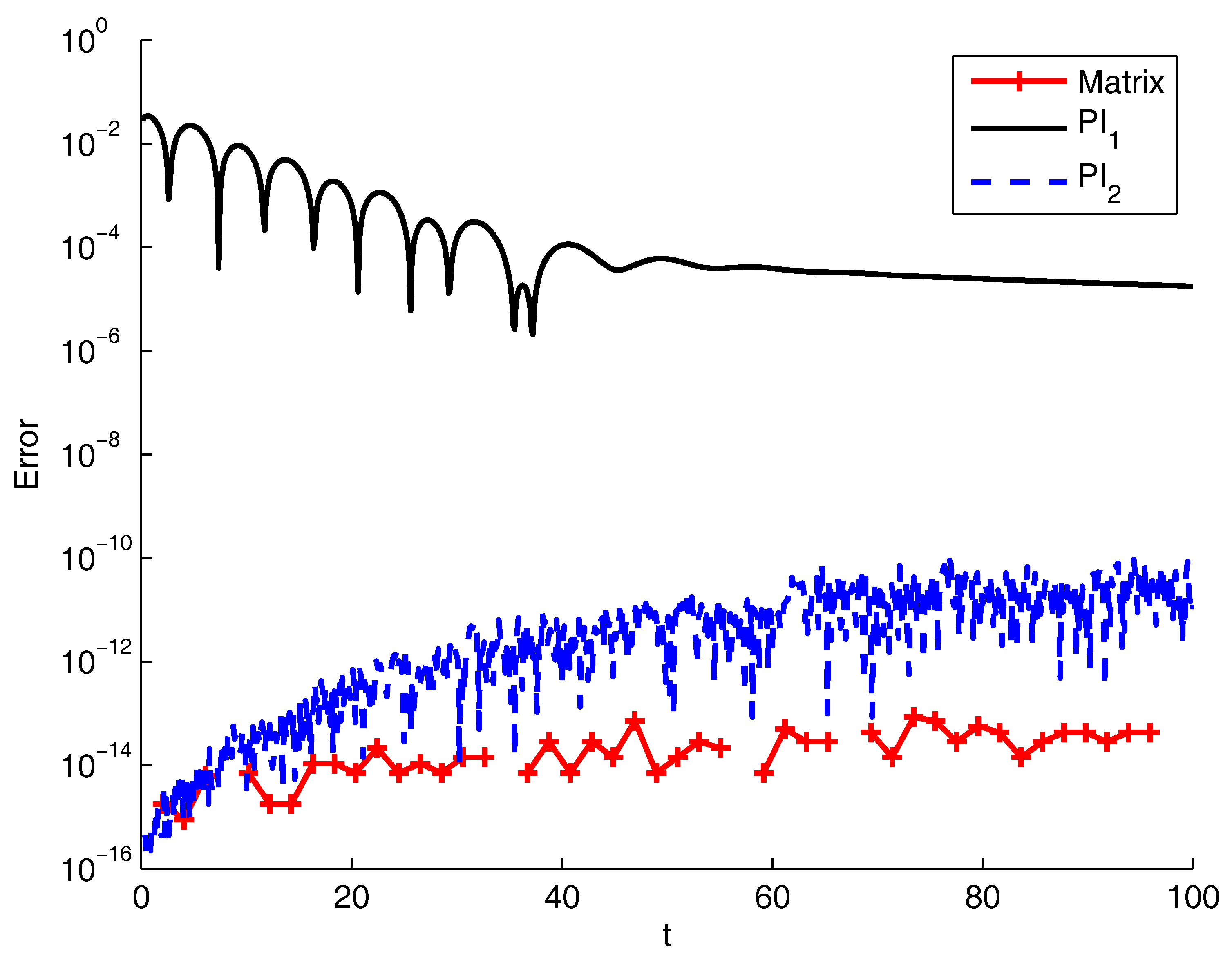
From Figure 1, we may appreciate the great accuracy of the matrix approach. PI₂ is also very accurate, particularly for small values of t, while PI₁ improves as t becomes larger but never reaches accuracies comparable to other methods. In terms of execution time,

Table 1. Comparison of execution time for the matrix approach and the product integration (PI) methods for computing the approximate solution at T.

T	Matrix	PI1	PI2
10	$5.4\times {10}^{-3}$	$\mathbf{3.0}\times {\mathbf{10}}^{-\mathbf{3}}$	$6.5\times {10}^{-3}$
50	$\mathbf{4.9}\times {\mathbf{10}}^{-\mathbf{3}}$	$1.6\times {10}^{-2}$	$3.1\times {10}^{-2}$
100	$\mathbf{4.0}\times {\mathbf{10}}^{-\mathbf{3}}$	$3.2\times {10}^{-2}$	$6.2\times {10}^{-2}$

shows that PI₁ and the matrix approach are similar for $T=10$, while the latter is more than 10 times faster for $T=50,100$.

4.2.2. The Basset Problem

The Basset equation is a classical model for the dynamics of a sphere immersed in an incompressible viscous fluid and subject to an elastic force. It was first considered by Basset in 1888, who interpreted the particle velocity relative to the fluid in terms of a fractional derivative of order $1/2$; this term is now called the Basset force. There are many studies on the Basset equation (see, e.g., [1,2,40,41,42]). Moreover, a generalization of the Basset force with fractional derivatives of order $0<\alpha <1$ is given by Mainardi [2].

The general equation is

$$\left[\frac{d}{dt}+{\delta }^{1-\alpha }\frac{d^{\alpha }}{d{t}^{\alpha }}+1\right]V\left(t\right)=1,V\left(0^{+}\right)=0,0<\alpha <1$$

(11)

The true solution of this problem is

$$V\left(t\right)=1-M(t;\alpha )$$

with $M(t;\alpha )$ to be determined by some inversion method. In particular, when $\alpha =p/q$, with $p,q$ being integer numbers and $p<q$, then

$${\displaystyle M(t;p/q)=\sum _{k=1}^q{C}_k{E}_{1/q}(a_k{t}^{1/q})}$$

where $a_1,a_2,\dots ,a_q$ are the zeros of the polynomial $P(x)=x^q+{\delta }^{(1-p/q)}{x}^p+1$, $A_k^{-1}={\prod }_{j=1}^q(a_k-a_j),$$j\ne k$ and $C_k=-A_k/a_k$ [40,41].

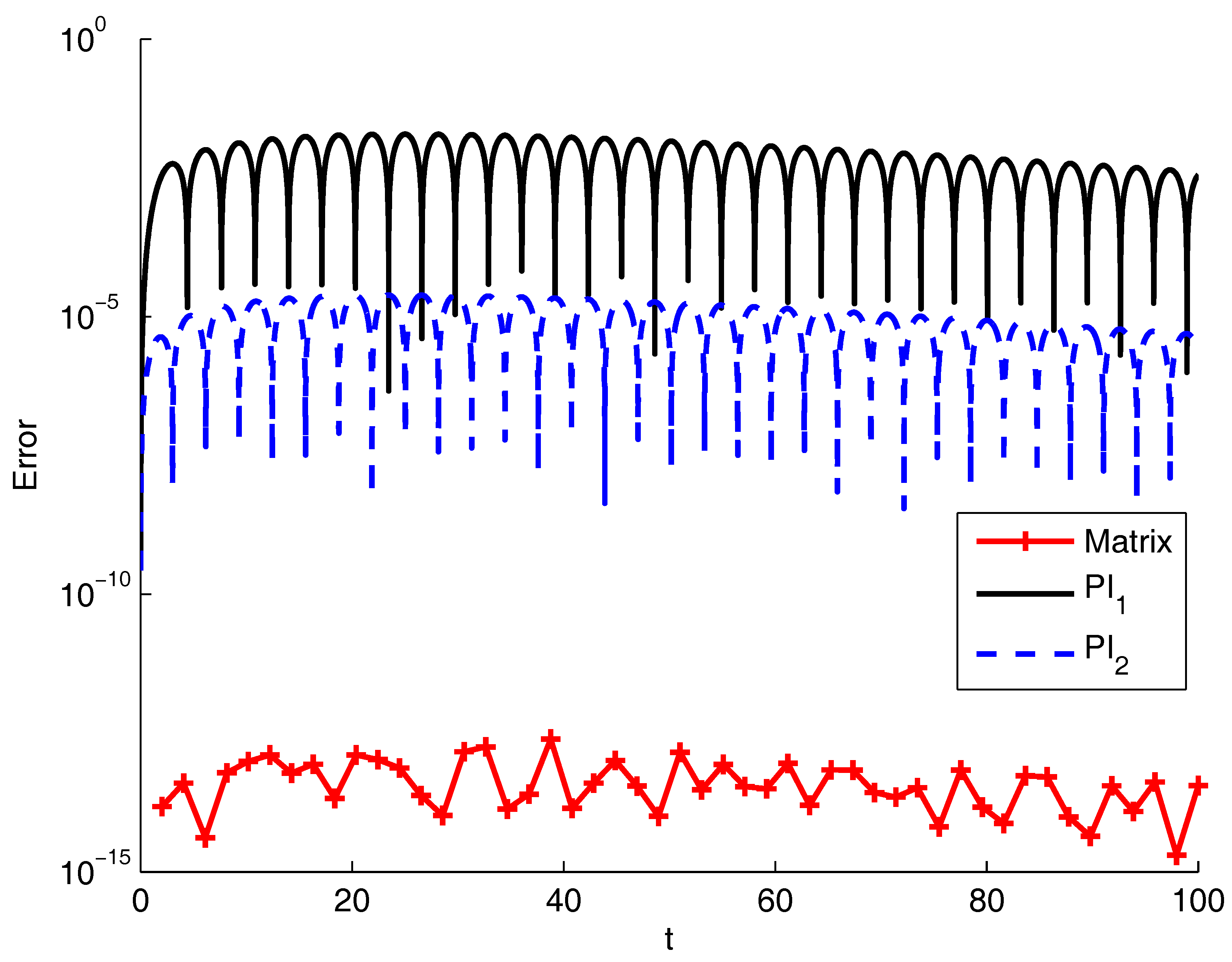
For our numerical tests, we considered $\alpha =1/2$, which results in the equivalent system of dimension $2\times 2$. We considered $\delta =9/(1+2\chi )$ with $\chi =10$, as in [2], and $h=2^{-4}$ for PI. For $\alpha =0.25$ and for other values of $\chi$, the results were very similar, and thus we omit their presentation.

Figure 2 reveals the excellent accuracy reached by the matrix approach. For this test, the method PI₂ was more accurate than PI₁, but it never caught the matrix approach. Moreover, the execution time was much longer, even 100 times greater than that of the matrix approach, as

Table 2. Comparison of execution time for the matrix approach and the product integration (PI) methods for computing the approximate solution at T for $\alpha =0.5$.

T	Matrix	PI1	PI2
10	$\mathbf{1.6}\times {\mathbf{10}}^{-\mathbf{3}}$	$6.3\times {10}^{-3}$	$1.2\times {10}^{-2}$
50	$\mathbf{1.6}\times {\mathbf{10}}^{-\mathbf{3}}$	$3.2\times {10}^{-2}$	$6.2\times {10}^{-2}$
100	$\mathbf{1.1}\times {\mathbf{10}}^{-\mathbf{3}}$	$6.1\times {10}^{-2}$	$1.3\times {10}^{-1}$

reports.

4.2.3. Fractional Oscillation Equation

The fractional oscillation equation is one of the basic examples to show the generalization of standard differential equations to fractional equations [2]. Its general form is

$$D^{\alpha }y\left(t\right)+{\omega }^{\alpha }y\left(t\right)=0$$

(12)

for $1<\alpha \le 2$ and $t\ge 0$. Two initial conditions are needed to uniquely solve this equation, namely, $y\left(0\right)$ and $y^{\prime }\left(0\right)$. If we assume that the latter is zero, the exact solution can be expressed in terms of the ML function:

$$y\left(t\right)=y\left(0\right)E_{\alpha ,1}(-{\left(\omega t\right)}^{\alpha })$$

As in [43], we consider $\alpha =1.95,\omega =1,y\left(0\right)=1,$ and $y^{\prime }\left(0\right)=0$. With this choice, the system corresponding to Equation (12) has dimension $N=39$. The step-size for PI is $h=2^{-7}$.

Figure 3 shows the error between the exact solution and the approximations given by the matrix approach and the PI methods. As for the previous examples, the matrix approach was definitely the most accurate and the fastest, as shown in

Table 3. Comparison of execution time for the matrix approach and the product integration (PI) methods for computing the approximate solution at T.

T	Matrix	PI1	PI2
10	$\mathbf{2.5}\times {\mathbf{10}}^{-\mathbf{2}}$	$4.4\times {10}^{-2}$	$8.9\times {10}^{-2}$
50	$\mathbf{2.7}\times {\mathbf{10}}^{-\mathbf{2}}$	$2.2\times {10}^{-1}$	$4.5\times {10}^{-1}$
100	$\mathbf{2.7}\times {\mathbf{10}}^{-\mathbf{2}}$	$4.4\times {10}^{-1}$	$9.0\times {10}^{-1}$

. Indeed, for the largest T value, the execution time for the PI₂ method was more than 30 times longer than that for the matrix approach.

4.2.4. Academic Examples

Example 1

We consider the MTFDE proposed in [44]:

$$D^{2}y\left(t\right)+D^{1/2}y\left(t\right)+y\left(t\right)=t^3+6t+\frac{3.2t^{2.5}}{\Gamma \left(0.5\right)},y\left(0\right)=0,y^{\prime }\left(0\right)=0$$

(13)

whose exact solution is $y\left(t\right)=t^3$.

The resulting matrix has dimension $2\times 2$. We use $h=2^{-3}$ for PI methods.

Figure 4 shows that the matrix approach was the most accurate for this test, even if PI₂ reached very high accuracies. However the former was the cheapest in terms of execution time, as

Table 4. Comparison of execution time for the matrix approach and the product integration (PI) methods for computing the approximate solution at T of Equation (13).

T	Matrix	PI1	PI2
10	$8.4\times {10}^{-3}$	$\mathbf{4.1}\times {\mathbf{10}}^{-\mathbf{3}}$	$7.3\times {10}^{-3}$
50	$\mathbf{9.5}\times {\mathbf{10}}^{-\mathbf{3}}$	$2.4\times {10}^{-2}$	$5.1\times {10}^{-2}$
100	$\mathbf{5.9}\times {\mathbf{10}}^{-\mathbf{3}}$	$3.7\times {10}^{-2}$	$7.3\times {10}^{-2}$

reports.

Example 2

We consider a test problem proposed in [19]. The FDE to solve is

$$D^{\alpha }y\left(t\right)+y\left(t\right)=t^m+\frac{m!}{\Gamma (m+1-\alpha )}{t}^{m-\alpha },y\left(0\right)=0,0<\alpha <1,m\in \mathbb{N}$$

(14)

whose exact solution is $y\left(t\right)=t^m$.

We use, as in [19], the values $m=4$ and $\alpha =0.4$. For the matrix approach, matrices of dimension $2\times 2$ come into play, while for the PI methods, we use $h=2^{-7}$.

The comments for the previous tests apply also for this case: from Figure 5 we may appreciate the excellent accuracy of the matrix approach while

Table 5. Comparison of execution time for the matrix approach and the product integration (PI) methods for computing the approximate solution at T for $\alpha =0.4$.

T	Matrix	PI1	PI2
10	$\mathbf{5.2}\times {\mathbf{10}}^{-\mathbf{3}}$	$8.1\times {10}^{-2}$	$1.6\times {10}^{-1}$
50	$\mathbf{4.7}\times {\mathbf{10}}^{-\mathbf{3}}$	$4.0\times {10}^{-1}$	$8.0\times {10}^{-1}$
100	$\mathbf{3.2}\times {\mathbf{10}}^{-\mathbf{3}}$	$7.9\times {10}^{-1}$	$1.6\times {10}^0$

reveals an even greater gap in terms of execution time, with a difference of 3 orders of magnitude between the matrix approach and PI₂.

References

- Gorenflo, R.; Mainardi, F. Fractional calculus: Integral and differential equations of fractional order. In Fractals and Fractional Calculus in Continuum Mechanics (Udine, 1996); Carpinteri, A., Mainardi, F., Eds.; Springer: Vienna, Austria, 1997; Volume 378, pp. 223–276. [Google Scholar]
- Mainardi, F. Fractional Calculus: Some Basic Problems in Continuum and Statistical Mechanics. In Fractals and Fractional Calculus in Continuum Mechanics (Udine, 1996); Carpinteri, A., Mainardi, F., Eds.; Springer: Vienna, Austria, 1997; pp. 291–348. [Google Scholar]
- Podlubny, I. Fractional differential equations. In Mathematics in Science and Engineering; Academic Press Inc.: San Diego, CA, USA, 1999; Volume 198. [Google Scholar]
- Diethelm, K. The Analysis of Fractional Differential Equations; Lecture Notes in Mathematics; Springer-Verlag: Berlin, Germany, 2010; Volume 2004. [Google Scholar]
- Mainardi, F. Fractional Calculus and Waves in Linear Viscoelasticity; Imperial College Press: London, UK, 2010. [Google Scholar]
- Lubich, C. Runge-Kutta theory for Volterra and Abel integral equations of the second kind. Math. Comput. 1983, 41, 87–102. [Google Scholar] [CrossRef]
- Lubich, C. Fractional linear multistep methods for Abel-Volterra integral equations of the second kind. Math. Comput. 1985, 45, 463–469. [Google Scholar] [CrossRef]
- Lubich, C. Discretized fractional calculus. SIAM J. Math. Anal. 1986, 17, 704–719. [Google Scholar] [CrossRef]
- Diethelm, K.; Ford, J.M.; Ford, N.J.; Weilbeer, M. Pitfalls in fast numerical solvers for fractional differential equations. J. Comput. Appl. Math. 2006, 186, 482–503. [Google Scholar] [CrossRef] [Green Version]
- Galeone, L.; Garrappa, R. Explicit methods for fractional differential equations and their stability properties. J. Comput. Appl. Math. 2009, 228, 548–560. [Google Scholar] [CrossRef]
- Garrappa, R. On some explicit Adams multistep methods for fractional differential equations. J. Comput. Appl. Math. 2009, 229, 392–399. [Google Scholar] [CrossRef]
- Garrappa, R.; Popolizio, M. On accurate product integration rules for linear fractional differential equations. J. Comput. Appl. Math. 2011, 235, 1085–1097. [Google Scholar] [CrossRef]
- Garrappa, R. Trapezoidal methods for fractional differential equations: Theoretical and computational aspects. Math. Comput. Simul. 2015, 110, 96–112. [Google Scholar] [CrossRef]
- Baleanu, D.; Diethelm, K.; Scalas, E.; Trujillo, J. Series on Complexity, Nonlinearity and Chaos. In Fractional Calculus: Models and Numerical Methods; World Scientific Publ: Singapore, 2012. [Google Scholar]
- Luchko, Y.; Gorenflo, R. An operational method for solving fractional differential equations with the Caputo derivatives. Acta Math. Vietnam. 1999, 24, 207–233. [Google Scholar]
- Diethelm, K.; Ford, N.J. Multi-order Fractional Differential Equations and Their Numerical Solution. Appl. Math. Comput. 2004, 154, 621–640. [Google Scholar] [CrossRef]
- Diethelm, K.; Luchko, Y. Numerical solution of linear multi-term initial value problems of fractional order. J. Comput. Anal. Appl. 2004, 6, 243–263. [Google Scholar]
- Luchko, Y. Initial-boundary-value problems for the generalized multi-term time-fractional diffusion equation. J. Math. Anal. Appl. 2011, 374, 538–548. [Google Scholar] [CrossRef]
- Garrappa, R. Stability-preserving high-order methods for multiterm fractional differential equations. Int. J. Bifurc. Chaos Appl. Sci. Eng. 2012, 22, 1250073. [Google Scholar] [CrossRef]
- Al-Refai, M.; Luchko, Y. Maximum principle for the multi-term time-fractional diffusion equations with the Riemann-Liouville fractional derivatives. Appl. Math. Comput. 2015, 257, 40–51. [Google Scholar] [CrossRef]
- Garrappa, R. Numerical Solution of Fractional Differential Equations: A Survey and a Software Tutorial. 2017; submitted. [Google Scholar]
- Esmaeili, S. The numerical solution of the Bagley-Torvik equation by exponential integrators. Sci. Iran. 2017, 2941–2951. [Google Scholar] [CrossRef]
- Torvik, P.; Bagley, R. On the appearance of the fractional derivative in the behavior of real materials. J. Appl. Mech. Trans. ASME 1984, 51, 294–298. [Google Scholar] [CrossRef]
- Mainardi, F. Fractional relaxation-oscillation and fractional diffusion-wave phenomena. Chaos Solitons Fractals 1996, 7, 1461–1477. [Google Scholar] [CrossRef]
- Diethelm, K.; Ford, J. Numerical Solution of the Bagley-Torvik Equation. BIT Numer. Math. 2002, 42, 490–507. [Google Scholar]
- Haubold, H.J.; Mathai, A.M.; Saxena, R.K. Mittag-Leffler functions and their applications. J. Appl. Math. 2011, 298628. [Google Scholar] [CrossRef]
- Gorenflo, R.; Kilbas, A.A.; Mainardi, F.; Rogosin, S. Mittag-Leffler functions. Theory and Applications; Springer Monographs in Mathematics; Springer: Berlin, Germany, 2014. [Google Scholar]
- Garrappa, R.; Popolizio, M. Evaluation of generalized Mittag–Leffler functions on the real line. Adv. Comput. Math. 2013, 39, 205–225. [Google Scholar] [CrossRef]
- Garrappa, R. Numerical evaluation of two and three parameter Mittag-Leffler functions. SIAM J. Numer. Anal. 2015, 53, 1350–1369. [Google Scholar] [CrossRef]
- Moret, I.; Novati, P. On the Convergence of Krylov Subspace Methods for Matrix Mittag–Leffler Functions. SIAM J. Numer. Anal. 2011, 49, 2144–2164. [Google Scholar] [CrossRef]
- Moret, I. A note on Krylov methods for fractional evolution problems. Numer. Funct. Anal. Optim. 2013, 34, 539–556. [Google Scholar] [CrossRef]
- Garrappa, R.; Popolizio, M. Computing the matrix Mittag-Leffler function with applications to fractional calculus. submitted.
- Cameron, R.F.; McKee, S. Product integration methods for second-kind Abel integral equations. J. Comput. Appl. Math. 1984, 11, 1–10. [Google Scholar] [CrossRef]
- Diethelm, K.; Freed, A.D. The FracPECE subroutine for the numerical solution of differential equations of fractional order; Forschung und wissenschaftliches Rechnen 1998; Heinzel, S., Plesser, T., Eds.; Gessellschaft für wissenschaftliche Datenverarbeitung: Goettingen, Germany, 1999; pp. 57–71. [Google Scholar]
- Diethelm, K.; Ford, N.J.; Freed, A.D. Detailed error analysis for a fractional Adams method. Numer. Algorithms 2004, 36, 31–52. [Google Scholar] [CrossRef]
- Garrappa, R.; Messina, E.; Vecchio, A. Effect of perturbation in the numerical solution of fractional differential equations. Discret. Contin. Dyn. Syst. Ser. B 2017. [Google Scholar] [CrossRef]
- Higham, N.J. Functions of matrices; Society for Industrial and Applied Mathematics (SIAM): Philadelphia, PA, USA, 2008. [Google Scholar]
- Garrappa, R.; Moret, I.; Popolizio, M. Solving the time-fractional Schrödinger equation by Krylov projection methods. J. Comput. Phys. 2015, 293, 115–134. [Google Scholar] [CrossRef]
- Garrappa, R.; Moret, I.; Popolizio, M. On the time-fractional Schrödinger equation: Theoretical analysis and numerical solution by matrix Mittag-Leffler functions. Comput. Math. Appl. 2017, 5, 977–992. [Google Scholar] [CrossRef]
- Mainardi, F.; Pironi, P.; Tampieri, F. A numerical approach to the generalized Basset problem for a sphere accelerating in a viscous fluid. In Proceedings of the 3rd Annual Conference of the Computational Fluid Dynamics Society of Canada, Banff, AB, Canada, 25–27 June 1995; Volume II, pp. 105–112. [Google Scholar]
- Mainardi, F.; Pironi, P.; Tampieri, F. On a generalization of the Basset problem via fractional calculus. In Proceedings of the 15th Canadian Congress of Applied Mechanics, Victoria, BC, Canada, 28 May–2 June 1995; Volume II, pp. 836–837. [Google Scholar]
- Garrappa, R.; Mainardi, F.; Maione, G. Models of dielectric relaxation based on completely monotone functions. Fract. Calc. Appl. Anal. 2016, 19, 1105–1160. [Google Scholar] [CrossRef]
- Edwards, J.T.; Ford, N.J.; Simpson, A.C. The numerical solution of linear multi-term fractional differential equations: Systems of equations. J. Comput. Appl. Math. 2002, 148, 401–418. [Google Scholar] [CrossRef]
- Ford, N.J.; Connolly, J.A. Systems-based decomposition schemes for the approximate solution of multi-term fractional differential equations. J. Comput. Appl. Math. 2009, 229, 382–391. [Google Scholar] [CrossRef]
Figure 1.
Error for the matrix approach and the product integration (PI) methods compared with the exact solution of the Bagley–Torvik equation. for PI.
Figure 2.
Error for the matrix approach and the product integration (PI) methods compared with the exact solution for for the Basset equation.
Figure 3.
Error for the matrix approach and the product integration (PI) methods compared with the exact solution for the fractional oscillation equation.
Figure 4.
Relative error for the matrix approach and the product integration (PI) methods compared with the exact solution for Equation (13).
Figure 5.
Relative error for the matrix approach and the product integration (PI) methods compared with the exact solution for for Equation (14).