Identifying the Informational/Signal Dimension in Principal Component Analysis


1
Dipartimento di Matematica, Sapienza Università di Roma, 00185 Roma, Italy
2
Departamento de Ecologia, Universidade Federal do Rio Grande do Sul, 91501-970 Porto Alegre, Brazil
*
Author to whom correspondence should be addressed.
Mathematics 2018, 6(11), 269; https://0-doi-org.brum.beds.ac.uk/10.3390/math6110269
Submission received: 23 October 2018
/
Revised: 11 November 2018
/
Accepted: 14 November 2018
/
Published: 20 November 2018
(This article belongs to the Special Issue New Paradigms and Trends in Quantitative Ecology)
Abstract
:The identification of a reduced dimensional representation of the data is among the main issues of exploratory multidimensional data analysis and several solutions had been proposed in the literature according to the method. Principal Component Analysis (PCA) is the method that has received the largest attention thus far and several identification methods—the so-called stopping rules—have been proposed, giving very different results in practice, and some comparative study has been carried out. Some inconsistencies in the previous studies led us to try to fix the distinction between signal from noise in PCA—and its limits—and propose a new testing method. This consists in the production of simulated data according to a predefined eigenvalues structure, including zero-eigenvalues. From random populations built according to several such structures, reduced-size samples were extracted and to them different levels of random normal noise were added. This controlled introduction of noise allows a clear distinction between expected signal and noise, the latter relegated to the non-zero eigenvalues in the samples corresponding to zero ones in the population. With this new method, we tested the performance of ten different stopping rules. Of every method, for every structure and every noise, both power (the ability to correctly identify the expected dimension) and type-I error (the detection of a dimension composed only by noise) have been measured, by counting the relative frequencies in which the smallest non-zero eigenvalue in the population was recognized as signal in the samples and that in which the largest zero-eigenvalue was recognized as noise, respectively. This way, the behaviour of the examined methods is clear and their comparison/evaluation is possible. The reported results show that both the generalization of the Bartlett’s test by Rencher and the Bootstrap method by Pillar result much better than all others: both are accounted for reasonable power, decreasing with noise, and very good type-I error. Thus, more than the others, these methods deserve being adopted.
1. Introduction
The definition of methods able to identify a suitable dimension of the representation space to consider for exploratory multidimensional analyses have been long investigated in the literature. In exploratory analysis, the inertia of a cloud of points is interpreted as its amount of information and it is usually split into additive components along orthogonal linear spaces, such as straights and planes. Thus, most methods sort dimensions according to the amount of information each may carry, which is the inertia along them, so that the first gather the most and very little usually results for the last ones. In general, limiting attention to the first few directions corresponds to the current practice, although not necessarily to the spirit of the exploratory analysis paradigm: indeed, the poor inertia attributed to an axis may not alone justify its drop—Gnanadesikan and Kettenring [1] stated that the last components may carry relevant informative power—unless one may clearly prove that their content is only noise, that is unstructured random variation. Thus, a stopping rule should mainly help in this crucial proof, but its use, even the best possible, could be either limiting or misleading, unless the information it provides is critically used in the study and not only to drop dimensions without care.
Dealing with Principal Component Analysis (PCA, [2,3,4]), several stopping rules have been developed thus far, all aiming at identifying a suitable dimension to which limit the study, supposing that they contain all the information relevant to the researcher. According to their rationale, they may be roughly classified into four classes: (1) thumb rules, based on empirical results; (2) parametric rules, based on statistical distributions; (3) distribution free rules, based on re-sampling; and (4) cross-validation rules, based on the goodness of fit of the solution to the original data. The first, such as Kaiser–Guttman [2,5,6] and scree-plot [7], have been severely criticized [2,8,9] for both their theoretical inconsistency and their poor performance, but are currently the most used in practice. Among the second, the Broken Stick method [10,11,12] and Bartlett’s [13] test are well appreciated. The distribution free methods were proved to perform much better than all others by Peres-Neto et al. [9]: for some of them confidence intervals or probabilities may be built via a Monte-Carlo simulation based on bootstrap or permutation re-sampling. Methods of cross-validation are discussed by Jolliffe [2]. They correspond to a modelling approach, which is the ability of a reduced-dimensional solution to rebuild sufficiently well the original data table. The methods of Wold [14] and Eastment and Krzanowski [15] are based on the improvement of an r-dimensional prediction in respect to an -dimensional one for each entry of the data table, obtained by excluding the original entry in the estimation process. Eventually, methods based on Bayesian statistics [16,17,18] have been developed in more recent years. Unfortunately, for the latter and for cross-validation rules prediction seems very complicated to implement, thus in our experimentation we considered only the method proposed by Pillar [19], which approaches the cross-validation framework.
Several studies and comparisons may be found in the literature (see, among others, the discussion in Jolliffe [2] and the experimentations carried out by both Jackson [8] and Peres-Neto et al. [9] with simulated data of known correlation structure and, more recently, Vieira [20]). In particular, in [9], computation-intensive re-sampling methods have been used among the many tested: these methods behaved much better than the others. These comparisons were carried out on simulated datasets whose known structure consisted in an a priori fixed correlation among the used variables: they defined a block structure of the correlation matrices, and set constant correlations between variables—higher within the same block and lower between different ones. This way, according to the correlation values, the block structure could result differently sharp. Then, random datasets with this correlation structure have been built, on which PCA was run and the stopping rules were applied. This method was adopted also by Caron [12] to study the Broken Stick rule and by Camiz and Pillar [21] to study the performance of methods to classify variables.
Both Jackson [8] and Peres-Neto et al. [9] considered the number of relevant principal components coincident with the number of the defined blocks and with respect to this number evaluated the stopping rules. Feoli and Zuccarello [22] discussed this relation in the extreme case of block matrices—that is, with zero correlation between blocks—but this does not seem consistent in general, because no theoretical relation a priori exists between factors and partially correlated blocks of correlated variables. Indeed, a block may be described by more than one factor, in particular with medium within blocks correlations, and the mix of low within blocks and high between blocks correlations makes unpredictable the PCA results, since their effects on the eigenstructure may not be known. Oppositely, as most methods deal with the eigenvalues, these are the most relevant elements that must be controlled in a comparison concerning different methods. For this reason, we propose here an alternative protocol, in which both the factorial structure and the introduced noise are clearly fixed, so that the stopping rule qualities may be more reliably checked. The new simulation protocol uses datasets of known eigenstructure and is applied in parallel to ten stopping rules, some of which were studied by Peres-Neto et al. [9].
We may consider two situations regarding finding the true dimension in principal component analyses: the need of a full reconstruction of a data table through orthogonal factors, such as in regression on principal components [23], that requires all the factors corresponding to non-zero eigenvalues, and the long-lasting study where factors are considered one by one and studied individually. In the latter case, starting from the factors that correspond to the largest eigenvalues, one proceeds asymptotically to interpret them and derives progressively some provisional conclusions, until no further interpretation may be found. This is achieved considering that the main factors correspond either to groups of variables with relevant nearly linear relations [2] or to variables independent from the others. Given the exploratory character of the analysis, in this recursive study, all possible interpretation helps are useful: the share of information progressively explained, the relations between the factors and both variables and units, the quality of partial reconstructions given by a limited number of factors, are all elements that contribute to form a thorough description of the data structure. In this context, the suggestion given by a stopping rule might corroborate the lack of a possible interpretation of the last dimensions, preventing a fanciful reconstruction or, on the opposite, encourage the search for a difficult interpretation that otherwise could be lost (see, e.g., [24]). This could be crucial, should the defined dimensions be used to carry out further analyses, such as confirmatory factor analysis or clustering on factor scores: in this case, one may risk to either introduce noise (overestimation) or lose information (underestimation) in the analysis, also causing distortion in the pattern of variation/covariation [25,26]. Nevertheless, since Karr and Martin [27] observed that the percentage of inertia attributed to principal components derived from real data may not be substantially greater than that derived from randomly generated ones, attention may not be limited only to the eigenvalues pattern, but other elements need to be considered seriously.
Moreover, there are frameworks, e.g., plant and/or animal community studies, in which PCA is mainly used to identify the main factors of variation. For these cases, it is claimed that 10–50% of a typical community inertia is considered noise [28], which is variation not particularly interesting for the study at hand. This is but one of the instrumental uses of PCA: in this case, the failure to distinguish between relevant data and noise may lead to the rejection of useful information, therefore limiting the understanding of ecological processes, or to attempt an interpretation of noise, driving to erroneous conclusions biased by essentially ecologically meaningless patterns [29]. Thus, situations exist in which a stopping rule may be important, especially when one deals with a sample. In this case, a suitable decision method might inform on the stability of the identified pattern across samples, an actually relevant issue when inference of results is forecast.
Unfortunately, in the quest for a stopping rule for PCA, we face terms such as “summarize most” of information, rebuild “at the best” the original table, “relevant” vs. “non-relevant” information, and “drop without damage”, i.e., terms whose consistency is poor. Indeed, even terms such as “signal” and “noise” or “error” may be misleading. In the following, we adopt two terms, signal and noise, to distinguish between what the researcher expects to identify and wishes to communicate as results of his/her work, and what does not add anything but individual random variation to what was found. In our experimentation, we define a data structure (the signal), we add noise to it and we check to what extent the methods under test are able to correctly distinguish between them.
2. Materials and Methods
2.1. Definition of Signal and Noise
The identification of the non-considered components—usually called residuals—with noise is far from the exploratory framework of PCA, in which the evaluation of the inertia explained by the chosen reduced dimensional solution is an indication of its relative relevance within the dataset but no more. Indeed, PCA transforms the original data matrix into another with the same rank—i.e., the same number of linearly independent characters—in which the columns are orthogonal to each other—thus, non-correlated—and ordered according to their relative importance—expressed as the share of inertia they are accounted for.
Consider a data table with n units and p characters. The PCA of may be fully described by the eigendecomposition of its associated correlation matrix. Given the real matrix of the standardized characters of , we derive and , the unit matrices of eigenvectors of and (the correlation matrix of ), respectively, and the diagonal matrix of the common eigenvalues. The new characters are valued on the units according to the columns of the matrix (the units’ coordinates) and their correlations with the old ones are given by the matrix . Indeed, as PCA is based on the Singular Value Decomposition (SVD, [30]), which states that , both its reconstruction formula
and the Eckart and Young [31] theorem ensure that the partial reconstruction , given by
is the best in the least-squares sense, on condition that the eigenvalues have been sorted in descending order. For this reason, it is current practice to limit attention to the first few dimensions, considering that the weight of each member of the sum in Equation (1) depends upon , supposed decreasing with increasing k. Thus, we may write
with , given by
a residual part not considered by the partial r-dimensional reconstruction of Equation (2). This led Peres-Neto et al. [9] to define as “non-trivial” the factors that carry relevant information and “trivial” the residuals, which are considered degenerate, thus carrying only noise. This is an erroneous consequence, since residuals in Equation (4) are not necessarily noise: the theorems simply state that their inertia is minimum and that the are centred and vary orthogonally with respect to the corresponding partial solution in Equation (2). It could be considered noise only if it would meet the ordinary assumptions, that is to be random variations around a theoretical model, independent, with zero expectation, equal variance and normally distributed: all issues that might be specifically ascertained.
We may better understand this issue if we compare these formulas with those of Factor Analysis [2,32]: in factor analysis the estimation of the is performed through a prefixed reduced number of factors usually but not always orthogonal, so that the model holds
with unit scores and factor loadings to be estimated and an error term that also accounts for specific variable’s variation [2], for which the ordinary assumptions (centered, independent, uncorrelated, and identically—hopefully normally—distributed) are expected. Unlike these, the are issued by Equation (4) and as such are in principle structured, so that they might be inspected in detail. Indeed, for this reason, the algorithm of factor analysis is different from that of PCA.
A tentative solution could be sought comparing the eigenvalues with those issued from a Wishart matrix, something analogous to either Malinvaud [33] or Ben Ammou and Saporta [34] tests for significance for single and multiple correspondence analysis, respectively. The Wishart’s is the covariance matrix of a set of independent normal random variables [35]. Regrettably, its use to identify a random component in the data, relegated to the least non-significant eigenvalues, seems in practice impossible (see the discussion in [6] Section 3.6).
In the case of PCA, the structure of the data table is investigated through either the covariance or the correlation matrices between the variables: in this paper, we limit our attention to correlation only, although the inference studies for PCA based on the covariance matrix do not apply to correlation [2,36,37]. This may be a limit for our study, but it corresponds to the most adopted way of using PCA.
An interesting alternative was found in the recent years, in which the data distribution requirements for the application of a specific statistics have been overcome by re-sampling techniques that allow simulating the distribution of the sought parameters based on the observed data [38,39]. The re-sampling techniques have been found useful in all situations in which either no known distribution would fit the data or a non-parametric test would be necessary. This is particularly relevant for PCA eigenvalues, whose distribution is not known. Efron and Tibshirani [40] studied the use of bootstrap in PCA context. Pillar [19] incorporated permutations into his Bootstrap method (see also Lebart et al. [4] for a discussion). We adopt it to check the significance of the results provided by the tested rules.
2.2. Stopping Rules
As already discussed, there are various types of stopping rules for PCA. Our choice among them depended either from their large use, their best performance according to previous tests, or because apparently they had never been compared to the others and could be easily implemented. The methods submitted to our test are described in the following. They are identified by acronyms (indicated within parentheses) to be used in the discussion of the results and in the graphics.
2.2.1. Kaiser–Guttman
The Kaiser-Guttman test (Guttman1 and Guttman07; [2]) is the most known thumb rule, based on the idea that, in PCAs based on a correlation matrix, only the principal components whose inertia is larger than the mean (that equals 1) should be considered, since they summarize more inertia than one original (standardized) variable. The assumptions are that a significant eigenvalue should be larger than a random one and that principal components should be a synthesis of more than one variable, a point of view more related to factor analysis, where factors common to all variables are sought, than to PCA. Jolliffe [2,6] criticized this idea, stating that a principal component not too much smaller than 1 may be very strongly correlated with one variable very different from the others, and thus it might not be ignored in an exploratory framework. Thus, he suggested paying attention even to eigenvalues larger than 0.7. We included this rule because it is largely adopted and we chose both 1.0 and 0.7 as thresholds to identify the data dimension according to this rule.
2.2.2. Broken Stick
The Broken Stick statistical test (BrokenStick; [41]) is based on the expected distribution of the lengths (in decreasing order) of p subintervals obtained by a random choice of cut-points of the real interval [41]. Frontier [10], see also [11] argued that the total inertia of a data table, should the eigenvalues be random, would be distributed according to these lengths in the same way, that is “broken down” into principal components similar to how a stick is randomly broken into p pieces. Thus, the absolute length of each piece relative to the whole (supposed to equal p, the number of eigenvalues), sorted in decreasing order, is expected to be
The rule establishes that every eigenvalue that is larger than the corresponding expected “broken” piece is non-random and thus the corresponding dimension a true piece of information. Indeed, this formula only depends upon the number of variables. In our test, each non-random eigenvalue was counted as signal.
2.2.3. Information Dimension
The Information Dimension method (Entropy; [42]) is based on information theory, i.e., on the measure of entropy of a set of real values, with the introduction of the (empirical) concept of information dimension. Entropy is commonly considered a distribution statistics for qualitative characters, for which the variance does not make sense. It is based on the relative frequencies of the supposed s levels of the character, giving . The entropy H ranges from 0, when only one level is present, thus (maximum order), to when the observations are equally distributed within the s levels (maximum disorder). As the eigenvalues sum up to the total inertia of the data table, the quantity may be taken as a relative frequency of inertia “units” along a PCA axis. Thus, the entropy is a measure of their scattering. As Cangelosi and Goriely [42] empirically found that the information dimension
approaches the geometrical dimension in some known cases, they suggested considering the highest integer smaller than as the number of informative dimensions. In fact, is the equivalent number of identical eigenvalues for the same value of H [43].
2.2.4. Rencher Bartlett-Kind Test
The Rencher Bartlett-Kind Test (Gen–Bartlett; [3]) is based on Bartlett [13] test for spherical distribution, which checks for significance the first eigenvalue only, thus ensuring that the data table at hand is non-random and worthy of consideration. Rencher [3] generalized this test, aiming at checking whether each sequential eigenvalue is significantly different from the remaining ones. The resulting test is based on the statistics for the kth eigenvalue, :
chi-square distributed with degrees of freedom. Thus, the dimension k is considered signal on condition that the chi-square test on the corresponding eigenvalue is significant at a specified probability threshold level.
2.2.5. Eigenvalues p-Value
This Eigenvalues p-Value test (Rnd-Lambda; [44]), together with the following three, may be considered distribution free. Apart from RVDim discussed in Section 2.2.7, no particular rationale was found in the literature, unless the choice to compare the found value with the empirical distribution obtained by parallel/randomization/permutation methods.
In this test, each eigenvalue is compared to the corresponding obtained from the data after random permutation of the values within each variable. If the p-value is significant, then its corresponding dimension is considered signal.
2.2.6. Pseudo-F Ratio
For each eigenvalue, the Pseudo-F Ratio test (Rnd-F; [45]) considers the ratio between the variance carried out in descending order by each dimension k and the residual attributed to the following :
hence its name. This pseudo-F is compared to the corresponding obtained through permutation. If the p-value is significant, then its corresponding dimension is considered signal. The high resemblance of this test with Dray’s test [26] described in the following must be noted.
2.2.7. RV Coefficient
As shown below, the RV Coefficient method (RVDim; [26]) is similar to the previous, but its building and its rationale deserve some attention for their meaning. Its understatement is that a relevant correlation between a matrix layer and the whole one could mean a major importance of the factor generating this layer with respect to the others.
The method checks step-by-step whether the kth one-dimensional layer in the adds non-random information to the already built -dimensional reconstruction: this is assumed by checking the ability of the kth layer to represent the residual of the said reconstruction. As a measure of reconstruction the index is used: first introduced by Escoufier [46] as a measure of (unsigned) correlation among vectors, it was later extended by Robert and Escoufier [47] to the case of matrices representing configuration or clouds of points in multidimensional spaces. The RV coefficient is based on the concept of sum of squares: given two matrices of coordinates of the same n units, and , both and are symmetrical matrices of scalar products between rows. As such, they summarized the relations existing among the units in each cloud in the space of representation. Thus, the coefficient
is a scalar product between and , that gives an overall measure of the relations existing between the two clouds of points analogous to covariance. Thus, the standardized coefficient
ranges and may be taken as unsigned correlation between and .
Dray [26] used RV and random permutations to check whether or not the contribution of every dimension to the reconstruction of the original data table, based on Eckart–Young singular value decomposition, may be considered relevant. For this task, he considered at each step the residual matrix in Equation (4) and computes through RV its correlation with its first layer to check if this may represent it significantly. What is noteworthy is that Dray proves that
with the singular values of . Thus, no important extra computation is needed to get it, and it results very similar to Rnd-F (Section 2.2.6). In addition, Josse et al. [48] proposed three approximations of the RV distribution that may be used to estimate its quantiles and thus avoid the time-consuming randomization. As we were using permutations for the other methods, we did not take advantage of this feature. If the p-value is significant, then its corresponding dimension is considered signal.
2.2.8. Random Average under Permutation
The Random Average under Permutation test (Avg-Rnd; [9]) consists on comparing each eigenvalue to the average of the corresponding ones generated under the permutation procedure described for Rnd-Lambda and Rnd-F, considering signal its dimension if it is larger than the average.
2.2.9. Bootstrap and Parallel Permutation
The Bootstrap and Parallel Permutation method (Bootstrap, [19]) aims at identifying the probability associated to the eigenvalues through the cross-correlation between the units’ coordinates issued by the PCA of the original data table and those issued from the bootstrapped samples. The algorithm steps are the following, once an probability threshold level is fixed for significance:
- Apply PCA to the original matrix , saving the resulting units’ coordinates in a matrix .
- Extract from the units set (the pseudo sampling universe in bootstrap re-sampling) a bootstrap sample of size , e.g., a data table , and submit it to PCA, obtaining a matrix of coordinates .
- Due to the nature of the bootstrap sampling (extraction of units with replacement, and thus possible repetition), the units in are a subset of . Thus, from , a matrix must be extracted, with the same units and in the same order of .
- For each dimension k of PCA, after a Procrustes adjustment [49] and using the first k principal components, compute the Pearson correlation between the coordinates of the kth principal components of and , respectively; the higher is this correlation, the better is the agreement between bootstrap and reference ordination and the more stable is its representation through the k-dimensional sample.
- Generate a matrix by randomly permuting the data within each variable of and repeat Steps 1–4 for this new matrix.
- Compare the correlation with the correlation obtained at Step 5.
- Repeat Steps 1–6 B times to get a p-value as the proportion of permutations for which resulted .
- Starting with the least ordination axis, and iterating towards the first one, a p-value suggests that this dimension is significantly more stable than the one found for the same dimension in the PCA of a random dataset. Thus, it is interpreted as signal.
- Once the kth dimension is deemed to carry signal, the test may stop and all larger dimensions are also taken into account, irrespective of their corresponding probabilities. Otherwise, the kth ordination dimension is considered noise, because it is both unstable and indistinguishable from an ordination of random data, and the probability of the next th axis is examined. See Pillar [19] for further details.
Two interesting features of Pillar’s method deserve being highlighted:
- As the comparison between real and bootstrapped data is performed considering the correlation among units’ coordinates, the method works with any kind of multidimensional scaling (including non-metric one) applied to any kind of data and resemblance measure. In addition, other measures of agreement, such as rank correlation, may be used instead.
- The bootstrap procedure to build the empirical probability of the obtained correlation may be repeated for the increasing size s of the bootstrapped sample, up to the table size n. This way the method is able to evaluate the sufficiency of the sample size, as it results by the stability of probabilities across increasing bootstrap sample sizes (as in [50]). Indeed, while increasing the sample size, should the probabilities associated to the kth dimension keep stable and larger than , this ordination axis is truly noise. Should they be decreasing, but still larger than even with a bootstrap sample of size n, this may be interpreted as the need of an even larger sample size to ensure that the ordination axis under examination is confirmed as either signal or noise.
In this work, due to our interest to compare PCA stopping rules by applying them to simulated data, we do not consider here these specific features, that are discussed in Pillar [19].
2.3. The Simulation
As our aim was to check to what extent a stopping rule is able to distinguish signal from noise, simulated data were generated by considering a deterministic structure, with known eigenvalues and eigenvectors, to which noise was added.
2.3.1. Data Generation
To generate data with a known eigenstructure, we applied the following iterative procedure:
- The eigenvalues of the simulated data are specified and normalized to sum up to their number.
- A data table is built with random numbers extracted from a specified distribution, representing a large number of units in rows and a specified number of variables in columns.
- The PCA of the data table is computed.
- The data table is reconstructed through Equation (1), substituting the eigenvalues issued by the PCA with the predefined ones.
- Steps 3 and 4 are iterated. This way the data table’s eigenvalues converge to the predefined ones, ensuring that the sum of the absolute differences between specified and resulting eigenvalues through iteration converges to zero. The procedure stops when the sum results less than a threshold, here fixed at
- A random sample with the specified number of units is extracted.
- Noise is added to the sample. It is a normally distributed random variable with zero mean and specified variance. The larger is the variance, the larger is the noise added to the defined eigenstructure. This way, to population zero-eigenvalues may correspond non-zero ones in the samples.
In our tests, we started from the idea that, in a PCA performed on a population, all non-zero eigenvalues are signal. In particular, zero eigenvalues appear when linear dependence exists among variables: in this case, the true dimension of the space in which the population cloud is embedded corresponds to the number of non-zero eigenvalues. Indeed, taking a non-noisy sample, its non-zero eigenvalues may differ from those of the population (they may also be zero), but none is an estimate of a zero eigenvalue of the population. On the other side, if we introduce artificially some noise, the noisy sample’s PCA would give the expected non-zero eigenvalues slightly modified and some random non-zero ones that are estimates of the zero-eigenvalues of the population. This means that the signal contained in the sample may be different but keep its dimension, whereas the noise could be identified by the non-zero estimates of the zero-eigenvalues. This is a new paradigm that we are using to check the performance of stopping rules. Indeed, they are correctly identifying this distinction between signal and noise, when they point the true population dimension.
2.3.2. The Experiment
We tested the stopping rules using simulated datasets composed of 9 variables with 11 pre-defined eigenstructures. Their relative proportions are shown in Table 1: their real values are obtained by multiplying them by 9, but this way it is easier to appreciate the different structures. Note that the true population dimension varies from 1 to 7, according to the non-zero eigenvalues, so that zero eigenvalues are expected to fill the gap to 9. The simulated data were prepared as follows:
- A population with 1000 units and 9 variables was generated with the procedure described in Section 2.3.1 with the specified eigenvalues.
- A sample with 30 units was randomly extracted from the population.
- To each simulated observation noise was added, extracted by a normally distributed random variable with zero mean and fixed variance.
- PCA was computed on the sample and the eigenvalues were sorted according to decreasing size.
- The ten methods were applied. For the distribution-free rules, each obtained statistics was compared to a number B of statistics obtained by applying the same method with the observations randomly permuted within each original variable. Then, a p-value for was calculated by the proportion of permutations for which resulted . If the p-value was smaller or equal than , it was considered significant and its corresponding dimension accounted for signal. Since and 1000 tests were applied in the following step, we set permutations, considering that in each distribution-free test this was enough to know whether .
- Steps (1)–(5) were repeated 1000 times for each of the 11 eigenstructures and each of nine fixed noise variances, ranging from 0 (no-noise) to 0.08 with step 0.01. For each repetition, a check was done whether the method correctly identified the expected dimension of the signal and treated the following as noise. This gave the proportion of correct answer for both power and type-I error, respectively.
- For each method, mean power and type-I error resulted for 99 combinations of 11 eigenstructures and 9 noise levels.
The procedures for data generation and testing of the stopping rules we describe here were implemented in the package MULTIV, coded in C++, with compiled versions available for download at http://ecoqua.ecologia.ufrgs.br/MULTIV.html. A script with the options chosen in MULTIV to carry out our experimentation is available as supplementary material S1 online.
3. Results
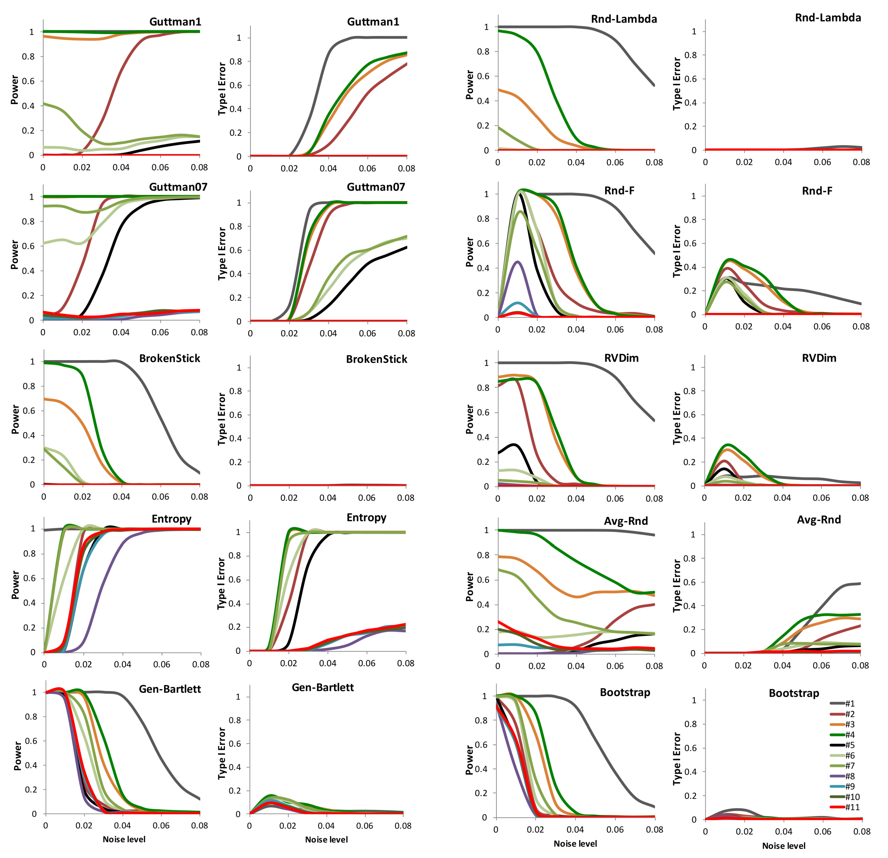
To report the results of the experiment, we consider of high interest the detailed study of the variation of both power and type-I error according to the different data tables’ eigenstructures and the increasing noise. They are all reported as supplementary material S2 online. For all methods at hand, we report in Figure 1, in Columns 1 and 3, the variation of power and, in Columns 2 and 4, the type-I error with respect to the increasing noise added to the simulated data for the different data structures. Actually, the reported power refers to the detection of the last dimension identified as signal and the type-I error refers to the first detection of noise. Here, we consider noise all the dimensions whose non-zero eigenvalues correspond to the zero-eigenvalues of the population, since they result essentially from the introduced noise. Thus, type-I error is a good measure of the methods’ quality with respect to the noise variation.
Looking at the power graphics (Figure 1, Columns 1 and 3), we identify five methods, BrokenStick, Gen–Bartlett, Rnd-Lambda, RVDim, and Bootstrap, whose power in general decreases regularly with the increase of noise: however, for some data structures, all these methods but Gen–Bartlett and Bootstrap show low power even with the least noise. Unlike these, Rnd-F presents a low power under zero noise, but then behaves similarly to the other methods. The behaviour of the remaining methods is strange: Guttman1, Guttman07, and Entropy increase their power with increasing noise, but this is limited to some eigenstructures only. Avg-Rnd shows a distinct behaviour compared to the other methods.
Looking at the type-I error graphics (Figure 1, Columns 2 and 4) we find two methods, BrokenStick and Rnd-Lambda, whose type-I error is in practice null in every case; then Gen–Bartlett, Bootstrap, RVDim, and Rnd-F show a uni-modal pattern, with a peak corresponding to the first level of non-zero noise. The peak is increasing from Gen–Bartlett to Rnd-F in this same order. Regarding the other methods, with increasing noise the type-I error sharply increases, but less with Avg-Rnd.
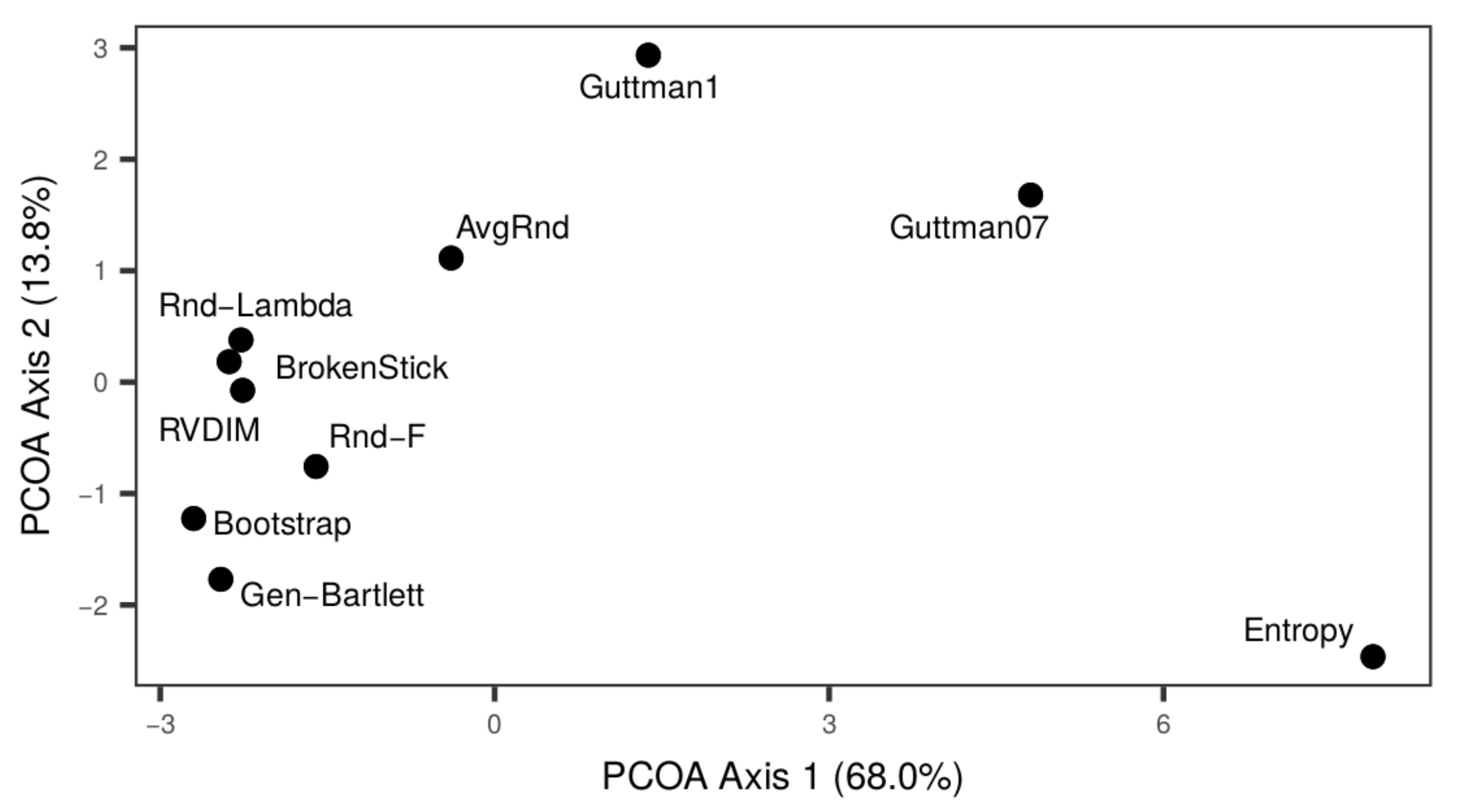
To summarize the results of the ten methods under examination, we applied Principal Coordinates Analysis (PCOA, [11]) to the results of the simulations for the 10 stopping rules, using 198 descriptors corresponding to both power for the last signal dimensions and type-I error for the first noise ones, in cross-reference to all levels of noise. In Figure 2, the ten methods are represented on its first principal plane: their reciprocal positions describe both their power and type-I error. Here, the pattern shows (from right to left on the first axis, but with an arch-effect involving the second one) Entropy, Guttman07, Guttman1, and Avg-Rnd are indeed the worst performing methods, especially in view of their increasing type-I error with increasing noise, followed by Rnd-Lambda, BrokenStick, RVDim, and Rnd-F, with good performance in terms of power and type-I error, and, on the higher end of the second axis, Bootstrap and Gen–Bartlett are the best performing in terms of both power and type-I error.
4. Discussion
The approach we adopted aimed at discriminating principal components with signal from those reflecting only noise. On one side, we examined known stopping rules for detecting the true dimensionality of a PCA and on the other we proposed an alternative way to test the methods at hand. In our opinion, the simulation of data with defined correlation structure as done in Peres-Neto, Jackson, and Somers [9] is not suitable for this kind of tests, since the number of identified components may result different from the number of correlation groups, in particular when the predefined differences of within and between groups correlations are low. This prevents a clear interpretation of the results, whose only conclusion may be that the ability to identify correctly supposedly non-random components and the proportion of erroneous detections of supposedly random ones are connected: the highest the power, the largest the type-I error, and vice-versa. Our method for data simulation, namely the a priori definition of the complete eigenstructure of the data and an explicit addition of noise, allows a much clearer definition of the true dimensionality given by the number of non-zero eigenvalues in the simulated population, and of the random components resulting from the added noise. This let us to compare the methods in a more suitable way, since the variation of the introduced noise could be considered consistently. Indeed, the behaviour of the methods at hand may be clearly checked and compared, in particular concerning the different basic data structures we used. Note also that these results could be graphically organized, with a better impact for the comprehension.
Our results allow identifying three groups of methods according to their general performance. In one group, formed by Entropy, Guttman07, Guttman1, and Avg-Rnd, the methods tend to monotonically increase both power and type-I error with increasing noise, for some data structures, which is a bad performance. Indeed, with increasing random noise, new dimensions are added, but since they are independent from each other and from the original non-zero dimensions, the new added dimensions should not become significant with increasing noise: on the opposite, this is not what these methods put in evidence. In a second group, formed by Rnd-lambda, BrokenStick, RVDim, and Rnd-F, better performances result, in particular, for type-I error. Indeed, the power reduces significantly with the raise of the noise in the data, but also very low (zero) power results for some data structures in the absence of noise, which is counter-intuitive. It must be pointed out that, unlike the others, two of these methods, Rnd-lambda and BrokenStick, show very low type-I error. In a third group, formed by Bootstrap, and Gen–Bartlett, the methods behave more predictably, with increasing noise while keeping reasonable the type-I error. Under low noise levels, these are the only methods that show consistently high power for all eigenstructure types; all other methods may show lower power depending on the eigenstructure type. In particular, as already pointed out, Rnd-F shows zero power under absence of noise. Further, no methods except Bootstrap and Gen–Bartlett are capable of detecting significant dimensions for eigenstructure type #10 with seven identical eigenvalues higher than zero and two zero ones. Except BrokenStick and Rnd-Lambda, which consistently show low type-I error, all methods show unimodal or sigmoidal response to increasing noise levels.
5. Conclusions
Applying the stopping rules based on the eigenvalues to routine data analysis may not prevent some possible misinterpretation, that might be avoided by carefully inspecting the results of a PCA. In particular, the inspection of the correlations between the original variables with the last dimensions and their quality of representation on them may help avoid the loss of some relevant information, such as some parts of variables explained mainly by small-inertia components. Another warning may concern the identification of outliers in the data: some of them may be found in the main dimensions and largely influence the principal axes formation. Conversely, others may be identified due to their good representation on the last axes while badly represented on the first ones. Both may be identified through their contribution to the components, something similar to the leverage in regression [30,51], and their quality of representation, usually concentrated in some dimension.
The reported results show that both Gen–Bartlett and Bootstrap perform much better than all others and, more than them, deserve being adopted. Note in particular the easiest implementation of Gen–Bartlett. Indeed, the tests prove only the quality of the examined methods to distinguish between signal and noise. In fact, no method based only on eigenvalues may do more. On the opposite, the Bootstrap may be preferred, because its check for stability, including the sample dimension, involves the eigenvalues but also the structure of the units’ coordinates on the principal components. In addition, it is likely that the presence of outliers may be detected in some way by Bootstrap, since they may cause instability in the results, depending on the reduced size subsampling.
The definition of simulated data based on a priori defined eigenstructure allows a true controlled introduction of noise and then a very clear distinction between expected signal and noise. In this case, the latter is relegated to the non-zero eigenvalues in the samples, which correspond to zero eigenvalues in the population. With this kind of experimentation, the behaviour of the examined methods may be made very clear and their evaluation is possible. Thus, our study may be followed by the examination of the methods based on cross-validation or on Bayesian statistics which, for the difficulty of their implementation, have been excluded from this survey: we refer in particular to the methods recently proposed by Auer and Gervini [17] and [52,53]. In addition, with a suitable choice of the eigenstructures of the simulated data, a study might be forecast to identify the gap between significant and non-significant eigenvalues necessary for a method to distinguish between them, a feature intrinsic in our study but not explicitly taken into account.
Supplementary Materials
The following are available online: S1 at https://0-www-mdpi-com.brum.beds.ac.uk/2227-7390/6/11/269/s1: script with the options chosen in MULTIV for generating simulated data and testing them stopping rules. S2 at https://0-www-mdpi-com.brum.beds.ac.uk/2227-7390/6/11/269/s2: Detailed results of the data simulation experiment.
Author Contributions
Conceptualization, S.C. and V.D.P.; Formal analysis, S.C. and V.D.P.; Methodology, S.C. and V.D.P.; Writing–original draft, S.C. and V.D.P.; Writing–review editing, S.C. and V.D.P.
Funding
This work started in the framework of the bilateral agreement between Sapienza Università di Roma and Universidade Federal do Rio Grande do Sul (UFRGS). It was then carried out and achieved during the stay of Sergio Camiz at Laboratório de Ecologia of UFRGS with a Special Visiting Researcher Fellowship under the Brazilian Scientific Mobility Program “Ciências sem Fronteiras” of CNPq, Brazil (Process number: 314443/2014-2). Also, Valério Pillar received support from CNPq (grant: 307689/2014-0). All institutions grants are kindly acknowledged.
Conflicts of Interest
The authors declare no conflict of interest.
References
- Gnanadesikan, R.; Kettenring, J. Robust estimates, residuals, and outlier detection with multiresponse data. Biometrics 1972, 28, 81–124. [Google Scholar] [CrossRef]
- Jolliffe, I. Principal Component Analysis; Springer: Berlin, Germany, 2002. [Google Scholar]
- Rencher, A.C. Methods of Multivariate Analysis; Wiley Interscience: New York, NY, USA, 2002. [Google Scholar]
- Lebart, L.; Piron, M.; Morineau, A. Statistique Exploratoire Multidimensionnelle—Visualisation et Inférence en Fouilles de Données; Dunod: Paris, France, 2016. [Google Scholar]
- Guttman, L. Some necessary conditions for common-factor analysis. Psychometrika 1954, 19, 149–161. [Google Scholar] [CrossRef]
- Jolliffe, I.T. Discarding Variables in a Principal Component Analysis. I: Artificial Data. Appl. Stat. 1972, 21, 160–173. [Google Scholar] [CrossRef]
- Cattell, R.B. The scree test for the number of factors. Multivar. Behav. Res. 1966, 1, 245–276. [Google Scholar] [CrossRef] [PubMed]
- Jackson, D.A. Stopping Rules in Principal Components Analysis: A Comparison of Heuristical and Statistical Approaches. Ecology 1993, 74, 2204–2214. [Google Scholar] [CrossRef]
- Peres-Neto, P.R.; Jackson, D.A.; Somers, K.M. How many principal components? stopping rules for determining the number of non-trivial axes revisited. Comput. Stat. Data Anal. 2005, 49, 974–997. [Google Scholar] [CrossRef]
- Frontier, S. Étude de la décroissance des valeurs propres dans une analyse en composantes principales: Comparaison avec le modèle du bâton brisé. J. Exp. Mar. Biol. Ecol. 1976, 25, 67–75. [Google Scholar] [CrossRef]
- Legendre, P.; Legendre, L. Numerical Ecology; Elsevier: Amsterdam, NY, USA, 1998. [Google Scholar]
- Caron, P.O. A Monte Carlo examination of the broken-stick distribution to identify components to retain in principal component analysis. J. Stat. Comput. Simul. 2016, 86, 2405–2410. [Google Scholar] [CrossRef] [Green Version]
- Bartlett, M.S. A note on the multiplying factors for various χ 2 approximations. J. R. Stat. Soc. Ser. B Math. 1954, 16, 296–298. [Google Scholar]
- Wold, S. Cross-validatory estimation of the number of components in factor and principal components models. Technometrics 1978, 20, 397–405. [Google Scholar] [CrossRef]
- Eastment, H.; Krzanowski, W. Cross-validatory choice of the number of components from a principal component analysis. Technometrics 1982, 24, 73–77. [Google Scholar] [CrossRef]
- Minka, T.P. Automatic choice of dimensionality for PCA. In Proceedings of the 13th International Conference on Neural Information Processing Systems, Vancouver, BC, Canada, 3–8 December 2001; pp. 598–604. [Google Scholar]
- Auer, P.; Gervini, D. Choosing principal components: A new graphical method based on Bayesian model selection. Commun. Stat. Simul. Comput. 2008, 37, 962–977. [Google Scholar] [CrossRef]
- Wang, M.; Kornblau, S.M.; Coombes, K.R. Decomposing the Apoptosis Pathway into Biologically Interpretable Principal Components. Cancer Inform. 2017, 17. [Google Scholar] [CrossRef] [Green Version]
- Pillar, V.D. The bootstrapped ordination re-examined. J. Veg. Sci. 1999, 10, 895–902. [Google Scholar] [CrossRef]
- Vieira, V.M. Permutation tests to estimate significances on Principal Components Analysis. Comput. Ecol. Softw. 2012, 2, 103–123. [Google Scholar]
- Camiz, S.; Pillar, V.D. Comparison of Single and Complete Linkage Clustering with the Hierarchical Factor Classification of Variables. Community Ecol. 2007, 8, 25–30. [Google Scholar] [CrossRef]
- Feoli, E.; Zuccarello, V. Fuzzy Sets and Eigenanalysis in Community Studies: Classification and Ordination are “Two Faces of the Same Coin”. Community Ecol. 2013, 14, 164–171. [Google Scholar] [CrossRef]
- Jolliffe, I.T. A note on the use of principal components in regression. J. R. Stat. Soc. Ser. C Appl. Stat. 1982, 31, 300–303. [Google Scholar] [CrossRef]
- Céréghino, R.; Pillar, V.; Srivastava, D.; de Omena, P.M.; MacDonald, A.A.M.; Barberis, I.M.; Corbara, B.; Guzman, L.M.; Leroy, C.; Bautista, F.O.; et al. Constraints on the Functional Trait Space of Aquatic Invertebrates in Bromeliads. Funct. Ecol. 2018, 32, 2435–2447. [Google Scholar] [CrossRef]
- Ferré, L. Selection of components in principal component analysis: A comparison of methods. Comput. Stat. Data Anal. 1995, 19, 669–682. [Google Scholar] [CrossRef]
- Dray, S. On the number of principal components: A test of dimensionality based on measurements of similarity between matrices. Comput. Stat. Data Anal. 2008, 52, 2228–2237. [Google Scholar] [CrossRef]
- Karr, J.; Martin, T. Random number and principal components: Further searches for the unicorn. In The Use of Multivariate Statistics in Wildlife Habitat; Capen, D., Ed.; United Forest Service: Washington, DC, USA, 1981; pp. 20–24. [Google Scholar]
- Gauch, H.G.J. Reduction by Eigenvector Ordinations. Ecology 1982, 63, 1643–1649. [Google Scholar] [CrossRef]
- Jackson, D.A.; Somers, K.M.; Harvey, H.H. Null models and fish communities: Evidence of nonrandom patterns. Am. Nat. 1992, 139, 930–951. [Google Scholar] [CrossRef]
- Abdi, H. Singular Value Decomposition (SVD) and Generalized Singular Value Decomposition (GSVD). In Encyclopedia of Measurement and Statistics; Salkind, N., Ed.; Sage: Thousand Oaks, CA, USA, 2007. [Google Scholar]
- Eckart, C.; Young, G. The approximation of one matrix by another of lower rank. Psychometrika 1936, 1, 211–218. [Google Scholar] [CrossRef]
- Basilevsky, A. Statistical Factor Analysis and Related Methods: Theory and Applications; Wiley-Blackwell: New York, NY, USA, 1994. [Google Scholar]
- Malinvaud, E. Data analysis in applied socio-economic statistics with special consideration of correspondence analysis. In Proceedings of the Academy of Marketing Science (AMS) Annual Conference, Bal Harbour, FL, USA, 27–30 May 1987. [Google Scholar]
- Ben Ammou, S.; Saporta, G. On the connection between the distribution of eigenvalues in multiple correspondence analysis and log-linear models. Revstat Stat. J. 2003, 1, 42–79. [Google Scholar]
- Wishart, J. The Generalised Product Moment Distribution in Samples from a Normal Multivariate Population. Biometrika 1928, 20, 32–52. [Google Scholar] [CrossRef]
- Anderson, T. Asymptotic Theory for Principal Component Analysis. Ann. Math. Stat. 1963, 34, 122–148. [Google Scholar] [CrossRef]
- Jackson, J.E. A User’s Guide to Principal Components; John Wiley & Sons: New York, NY, USA, 1991. [Google Scholar]
- Efron, B. Bootstrap methods: Another look at jackknife. Ann. Stat. 1979, 7, 1–26. [Google Scholar] [CrossRef]
- Manly, B.F. Randomization, Bootstrap and Monte Carlo Methods in Biology; Texts in Statistical Science; Chapman & Hall/CRC Press: Boca Raton, FL, USA, 2007. [Google Scholar]
- Efron, B.; Tibshirani, R. An Introduction to the Bootstrap; Chapman and Hall: New York, NY, USA, 1993. [Google Scholar]
- Barton, D.; David, F. Some notes on ordered random intervals. J. R. Stat. Soc. Ser. B Methodol. 1956, 18, 79–94. [Google Scholar]
- Cangelosi, R.; Goriely, A. Component retention in principal component analysis with application to cDNA microarray data. Biol. Direct 2007, 2, 1–21. [Google Scholar] [CrossRef] [PubMed]
- Jost, L. Entropy and diversity. Oikos 2006, 113, 363–375. [Google Scholar] [CrossRef]
- Ter Braak, C.J. CANOCO—A FORTRAN Program for Canonical Community Ordination by [Partial][Detrended][Canonical] Correspondence Analysis, Principal Components Analysis and Redundancy Analysis (Version 2.1); Technical Report; Agricultural Mathematic Group: Wageningen, The Netherlands, 1988. [Google Scholar]
- Ter Braak, C.J. CANOCO Version 3.1, Update Notes; Technical Report; Agricultural Mathematics Group: Wageningen, The Netherlands, 1990. [Google Scholar]
- Escoufier, Y. Le Traitement des Variables Vectorielles. Biometrics 1973, 29, 751–760. [Google Scholar] [CrossRef]
- Robert, P.; Escoufier, Y. A Unifying Tool for Linear Multivariate Statistical Methods: The RV-Coefficient. Appl. Stat. 1976, 25, 257–265. [Google Scholar] [CrossRef]
- Josse, J.; Pagès, J.; Husson, F. Testing the significance of the RV coefficient. Comput. Stat. Data Anal. 2008, 53, 82–91. [Google Scholar] [CrossRef]
- Schönemann, P.H.; Carroll, R.M. Fitting one matrix to another under choice of a central dilation and a rigid motion. Psychometrika 1970, 35, 245–255. [Google Scholar] [CrossRef]
- Pillar, V.D. Sampling sufficiency in ecological surveys. Abstr. Bot. 1998, 22, 37–48. [Google Scholar]
- Stapleton, J. Linear Statistical Models; Wiley: New York, NY, USA, 1995. [Google Scholar]
- Camacho, J.; Ferrer, A. Cross-validation in PCA models with the element-wise k-fold (ekf) algorithm: Theoretical aspects. J. Chemom. 2012, 26, 361–373. [Google Scholar] [CrossRef] [Green Version]
- Camacho, J.; Ferrer, A. Cross-validation in PCA models with the element-wise k-fold (ekf) algorithm: Practical aspects. Chemom. Intell. Lab. Syst. 2014, 131, 37–50. [Google Scholar] [CrossRef] [Green Version]
Figure 1.
Experiment results. The graphics represent the power and type-I error of the ten stopping rules for PCA in defining both signal and noise dimensions under increasing levels of added noise (horizontal axis), considering nine variables with normal distribution and sample size of 30 units. The coloured lines correspond to the eigenstructures of the simulated datasets defined in Table 1. Columns 1 and 3: Graphs for power, referring to the last signal dimension. Columns 2 and 4: Graphs for type-I error, referring to the first noise one.

Figure 2.
Ordination of the 10 stopping rules based on their performance. Each method was described by a total of 198 descriptors, which corresponded to the power and type-I error using different options for simulated data generation: sample size of 30 units, 11 eigenstructures (see Table 1) and 9 increasing levels of introduced noise (starting from zero). Power was the proportion of simulated data in which the last informative dimension in the specified eigenstructure was detected as relevant by the stopping rule. Type-I error is the proportion in which the first residual dimension was (wrongly) detected as information by the stopping rule. For this graphic, Principal Coordinates Analysis based on Euclidean distances between methods was used. Axes 1 and 2 are accounted for 68.0% and 13.8% of total inertia, respectively. See main text for the description of the stopping rules.


Table 1.
Relative proportions of eigenvalues of the 11 simulated data structures used for testing the stopping rules prior the introduction of noise. In the last columns, the true dimension of the data and the ratio between the first and the last non-zero eigenvalues are shown. The eigenvalues of the noise-free data structures correspond to these proportions multiplied by 9.
| Eigen | Specified Eigenvalues (Proportions) | TrueDim | Ratio | ||||||||
|---|---|---|---|---|---|---|---|---|---|---|---|
| #1 | 1 | 0 | 0 | 0 | 0 | 0 | 0 | 0 | 0 | 1 | 1.0 |
| #2 | 0.810 | 0.140 | 0.050 | 0.000 | 0.000 | 0.000 | 0.000 | 0.000 | 0.000 | 3 | 16.1 |
| #3 | 0.545 | 0.273 | 0.182 | 0.000 | 0.000 | 0.000 | 0.000 | 0.000 | 0.000 | 3 | 3.0 |
| #4 | 0.416 | 0.315 | 0.268 | 0.000 | 0.000 | 0.000 | 0.000 | 0.000 | 0.000 | 3 | 1.6 |
| #5 | 0.568 | 0.201 | 0.109 | 0.071 | 0.051 | 0.000 | 0.000 | 0.000 | 0.000 | 5 | 11.2 |
| #6 | 0.359 | 0.221 | 0.167 | 0.136 | 0.117 | 0.000 | 0.000 | 0.000 | 0.000 | 5 | 3.1 |
| #7 | 0.251 | 0.211 | 0.191 | 0.178 | 0.168 | 0.000 | 0.000 | 0.000 | 0.000 | 5 | 1.5 |
| #8 | 0.386 | 0.193 | 0.129 | 0.096 | 0.077 | 0.064 | 0.055 | 0.000 | 0.000 | 7 | 7.0 |
| #9 | 0.225 | 0.170 | 0.145 | 0.129 | 0.118 | 0.110 | 0.103 | 0.000 | 0.000 | 7 | 2.2 |
| #10 | 0.181 | 0.157 | 0.145 | 0.137 | 0.131 | 0.126 | 0.122 | 0.000 | 0.000 | 7 | 1.5 |
| #11 | 0.143 | 0.143 | 0.143 | 0.143 | 0.143 | 0.143 | 0.143 | 0.000 | 0.000 | 7 | 1.0 |
© 2018 by the authors. Licensee MDPI, Basel, Switzerland. This article is an open access article distributed under the terms and conditions of the Creative Commons Attribution (CC BY) license (http://creativecommons.org/licenses/by/4.0/).
Share and Cite
MDPI and ACS Style
Camiz, S.; Pillar, V.D. Identifying the Informational/Signal Dimension in Principal Component Analysis. Mathematics 2018, 6, 269. https://0-doi-org.brum.beds.ac.uk/10.3390/math6110269
AMA Style
Camiz S, Pillar VD. Identifying the Informational/Signal Dimension in Principal Component Analysis. Mathematics. 2018; 6(11):269. https://0-doi-org.brum.beds.ac.uk/10.3390/math6110269
Chicago/Turabian StyleCamiz, Sergio, and Valério D. Pillar. 2018. "Identifying the Informational/Signal Dimension in Principal Component Analysis" Mathematics 6, no. 11: 269. https://0-doi-org.brum.beds.ac.uk/10.3390/math6110269
Note that from the first issue of 2016, this journal uses article numbers instead of page numbers. See further details here.