Efficient Solutions of Interval Programming Problems with Inexact Parameters and Second Order Cone Constraints

1
Department of Mathematics, Faculty of Mathematical Sciences and Computer, Shahid Chamran University of Ahvaz, 6135743136 Ahavaz, Iran
2
Faculty of Mathematical Sciences, Sharif University of Technology, 11365-11155 Tehran, Iran
*
Authors to whom correspondence should be addressed.
Mathematics 2018, 6(11), 270; https://0-doi-org.brum.beds.ac.uk/10.3390/math6110270
Submission received: 1 October 2018
/
Revised: 5 November 2018
/
Accepted: 13 November 2018
/
Published: 20 November 2018
Abstract
:In this article, a methodology is developed to solve an interval and a fractional interval programming problem by converting into a non-interval form for second order cone constraints, with the objective function and constraints being interval valued functions. We investigate the parametric and non-parametric forms of the interval valued functions along with their convexity properties. Two approaches are developed to obtain efficient and properly efficient solutions. Furthermore, the efficient solutions or Pareto optimal solutions of fractional and non-fractional programming problems over are also discussed. The main idea of the present article is to introduce a new concept for efficiency, called efficient space, caused by the lower and upper bounds of the respective intervals of the objective function which are shown in different figures. Finally, some numerical examples are worked through to illustrate the methodology and affirm the validity of the obtained results.
MSC:
90C46; 90C291. Introduction
We consider solving fractional interval programming problems with second order cone constraints with both the objective and constraints being interval valued functions. There are several approaches in the literature to solve such problems. Nonlinear interval optimization problems have been studied in several directions by many researchers during the past few decades [1,2,3,4]. Most considered models used quadratic programming problems with interval parameters. A methodology applied to interval valued convex quadratic programming problems by Bhurjee and Panda [1] which categorized how a solution of a general optimization problem can exist.
In the past few decades, fractional programming problems have also attracted the interest of many researchers. These problems have applications in the real physical world such as finance, production planning, electronic, etc. Fractional programming is being used for modelling real life problems involving one or more objective(s) such as actual cost/standard cost, inventory/sales and profit/cost. There are different algorithms to determine solutions of particular fractional programming problems. For example, Charnes and Cooper [5] converted a linear fractional program (LFP) to a linear program (LP) by a variable transformation technique. Tantawy [6] proposed an iterative method based on a conjugate gradient projection method. Dinkelbach [7] considered the same objective over a convex feasible set. He also solved the same problem using a sequence of nonlinear convex programming problems.
On the other hand, we know that the convexity of the SOCP (Second Order Cone Constraints) problems are definite. The problems such as linear programs, convex quadratic programs and quadratically constrained convex quadratic programs can be easily converted to SOCP problems; for several other types of problems not falling into these three categories, see [8,9].
Lobo et al. [9] discussed several applications of SOCP in engineering. Nesterov and Nemirovski [10] and Lobo et al. [9,11] showed several kinds of problems formulated as SOCP problems, such as filter design, truss design, grasping force optimization in robotics, etc. In a pioneering paper, Nesterov and Nemirovski [10] applied the concept of self-concordant barrier to SOCP problems and found an iteration complexity of for problems with m second order cone inequalities.
Nestrov and Todd [12,13] were the first to investigate primal-dual interior methods for SOCP problems in which they investigate their outcome in the form of optimization over self-scaled cones having second order cones class as an especial case. Alizadeh & Goldfarb [8] considered and overviewed a large class of SOCP problems. They showed that many optimization problems such as linear programming (LP), quadratic programming (QP), quadratically constrained quadratic programming (QCQP) and other types of optimization problems could be rewritten as SOCP problems. They also demonstrated the method of converting different types of constraints into the form of SOC inequalities. Furthermore, they described an algebraic foundation of SOCs and showed how robust least squares and robust linear programming problems could be converted to SOCPs. The authors of [8] also discussed duality and complementary slackness for SOCP with notions of primal and dual non-degeneracy and strict complementarity along with logarithmic barrier function and primal-dual path following interior point methods (IPMs) for SOCPs.
Kim and Kojima [14] showed that semi-definite programming (SDP) and SOCP relaxation provide exact optimal solutions for a class of non-convex quadratic optimization problems. Moreover, SDP problems can in fact be formulated as SOCP problems and solved as such. There are a number of advantages for an SOCP problem. Adding a SOC constraint sometimes leads to negative decision variables, which usually does not occur with LP problems unless we let the variables be free in sign and usually get a much better solution, even though the dimension and convexity remain the same.
In our work here, we establish two results concerning efficient and properly efficient solutions of interval programming problems constrained with a second order cone constraint. The remainder of our work is organized as follows. In Section 2, the definitions and notations are provided. The interval valued functions in parametric and non-parametric forms along with their convexity properties are discussed in Section 3. In Section 4, we explain the existence of solutions for interval valued optimization problems and establish certain results concerning the efficient and properly efficient solutions of the interval problems involving SOC constraints. We also investigate the efficient solution for interval fractional and non-fractional programming problems in . In Section 5, some numerical examples are worked through to verify the results on efficient and properly efficient solutions using MATLAB software environment. We conclude in Section 6.
2. Definitions and Notations
Let be represented as the class of all closed intervals. A closed interval is shown by , where and are respectively the lower and upper bounds of . For closed intervals M, N, and we have:
- (i)
- ,
- (ii)
- ,
- (iii)
- .
Definition 1.
If and are bounded, real valued intervals, then the multiplication of M and N is defined to be
Let be a closed interval in R, for each . The interval-valued function F may be represented as , where and are real-valued functions defined on and satisfy , for every . We say that the interval-valued function F is differentiable at if and only if the real-valued functions and are differentiable at . To know more, see [2].
Let and be two closed intervals in R and the relation “⪯” be a partial ordering on . We write if and only if and . We also write if and only if and , meaning that M is inferior to N, or N is superior to M.
A second order cone is defined as follows:
where is the standard Euclidean norm, and n is the dimension of ; n is usually dropped from the subscript. We refer to inequality as the second-order cone inequality.
For the cone Q, let
denote the boundary of Q without the origin 0. In addition, let
denote the interior of Q.
We continue to present an overview of the SOCP problem. A standard form of an SOCP problem is given by
with its dual being
where m is the number of blocks, is the dimension of the problem, and [8].
We make the following assumptions regarding the primal-dual pair and [8].
Assumption 1.
The matrix has r linearly independent rows.
Assumption 2.
Due to the strict feasibility of both primal and dual, there exists a vector for every , for , and dual-feasible y and such that for .
Remark 1.
If problem has only one second order cone constraint, then the standard SOCP problem can be written as
with its corresponding dual as
Over time, we have seen a rapid development in improvement of software packages that can be applied to the problems such as SOCPs and mixed SOCP problems. SeDuMi [11] is a widely available package based on the Nesterov–Todd method.
3. Interval Valued Function
The definition of interval function in terms of functions of one and more intervals is given by see [2,3,4]. Walster and Hansen and Moore [2] defined an interval function as a function of one or more interval arguments onto an interval. Wu considered the interval valued function as where
These functions may be defined on one or more interval arguments or maybe interval extension of real valued functions. The interval valued function in parametric form, introduced by [4], is as follows. For , let . Then, for a given interval vector , an interval valued function is defined
For every fixed x, if is continuous in then and exist. Then,
If is linear in then and exist. If is monotonically increasing in then
3.1. Interval Valued Convex Function
Interval valued convex function has the important property to guarantee the existence of solution of the interval optimization problem.
Definition 2.
[4] An interval valued function is said to be convex regarding ⪯ on a convex set if for every and we have
Remark 2.
From Definition 2, one may observe that is convex regarding meaning that
for all ; we can realize that is convex with respect to ⪯ iff is a convex function on for every t.
3.2. Interval Valued Function in the Parametric Form
Let a binary operation on the set of real numbers be represented by . The binary operation ⊛ between two intervals and in , denoted by , is the set In the case of division, it is to be noted that An interval may be shown as a parameter form in several disciplines. Any point in M may be expressed as , where . Throughout our work, we consider a specific parametric representation of an interval as The algebraic operations over classical intervals can be represented as either lower or upper bounds of the intervals [1]. The parametric form of interval operations can be represented as follows:
In addition, can be expressed in terms of parameters as
where
4. Existence of Solutions
In this section, we consider the interval optimization problem as follows:
where and the interval valued functions are the sets and
Discussion of the partial ordering is seen in Section 2, and the feasible space of is expressed as the following set:
Definition 3.
is said to be an efficient solution of if there does not exist any with and [4].
Definition 4.
is said to be a properly efficient solution of (P3), if is an efficient solution and there exists a real number such that for some and all with , at least there is one , exists with and
Consider the following optimization problem with respect to a weight function
where . Here, are mutually independent and each varies from 0 to 1. Thus, is a function of x only, say . Thus, as is a general nonlinear programming problem free from interval uncertainty. The problem can be solved by a nonlinear programming technique. The following theorem establishes the relationship between the solution of the transformed problem and the original problem [4].
Theorem 1.
If is an optimal solution of , then is a properly efficient solution of .
Proof.
See [4]. ☐
4.1. Alternative Method for Solving an Interval Problem with an SOC Constraint
Here, we consider a problem by applying the order relation “⪯” for the constraints as follows:
where the are interval-valued constraints. A point is a feasible solution of problem if for or equivalently, and , for . Then, the auxiliary interval-valued optimization problem can be rewritten as follows:
It is obvious that the feasible regions of problems and are the same and, since their objective function is also the same, we have the same solution for both problems. The interval property of problem incurs a very important concept called efficient space which is a new concept from the optimization point of view.
Therefore, the interval-valued optimization problem is easily converted to a common form as below:
where is an interval-valued function, and and are real-valued functions. Let and be two closed intervals in R. We write if and only if and and we write iff and . Equivalently, iff
We need to interpret the meaning of minimization for . Since ⪯ is a partial ordering, not a total ordering on , we may follow the similar solution concept (efficient solution) used in multi-objective programming problem to interpret the meaning of minimization in the primal problem . For the minimization problem , we say that the feasible solution is better than (dominates) the feasible solution if . Therefore, we propose the following definition.
Definition 5.
Let be a feasible solution of the primal problem . We say that is an efficient solution of if there exists no such that . In this case, is called the efficient objective value of F.
We denote the set of all efficient objective values of problem by . More precisely, we write
where is an efficient solution of Let m be a real number. Then, it can be represented as an interval . Let be a closed interval. By , we mean .
Now, consider the following optimization problem:
Obviously, if is an optimal solution of problem , then is a nondominated solution of problem see [4]. We may now focus here on the two results given as Theorems 2 and 3 below, by which the optimal solutions of the problems and are indeed the efficient solutions of the problem :
where and are positive scalars.
Theorem 2.
If is an optimal solution of problem , then is an efficient solution of problem .
Proof.
We see that problems and have the same feasible region. Suppose that is not an efficient solution. Then, there exists a feasible solution x such that . From inequation (1), it means that
This also shows that , which contradicts the fact that is an optimal solution of problem . This completes the proof. ☐
Theorem 3.
If is an optimal solution of problem , then is an efficient solution of problem .
Proof.
We see that problems and have the same feasible region. Suppose that is not an efficient solution. Then, there exists a feasible solution x such that . From (1), it means that
Then, we have
This also shows that , which contradicts the fact that is an optimal solution of problem . This completes the proof. ☐
4.2. Interval Valued Convex Linear Programming Problem with SOC Constraint
An interval valued optimization problem (P3) is said to be an interval valued convex programming problem, if and are convex functions with respect to
If (P3) is an interval valued convex programming problem, then is a convex programming problem.
A general interval linear programming problem (P3) has the following form:
where and is an interval valued matrix with and the product of a real vector and an interval vector .
5. Numerical Results
In this section, we consider three examples having various dimensions to illustrate the obtained results. In order to solve problems using both theorems, we use the fmincon command of Matlab. Notations are given in Table 1 and the results are summarized in Table 2, Table 3 and Table 4 and the corresponding diagrams. We generate problems with different dimensions and report the required CPU times. All computations are performed on MATLAB R2015a (8.5) using a laptop with Intel(R) Core i3 CPU 2.53 GHz and 5.00 GB of RAM.
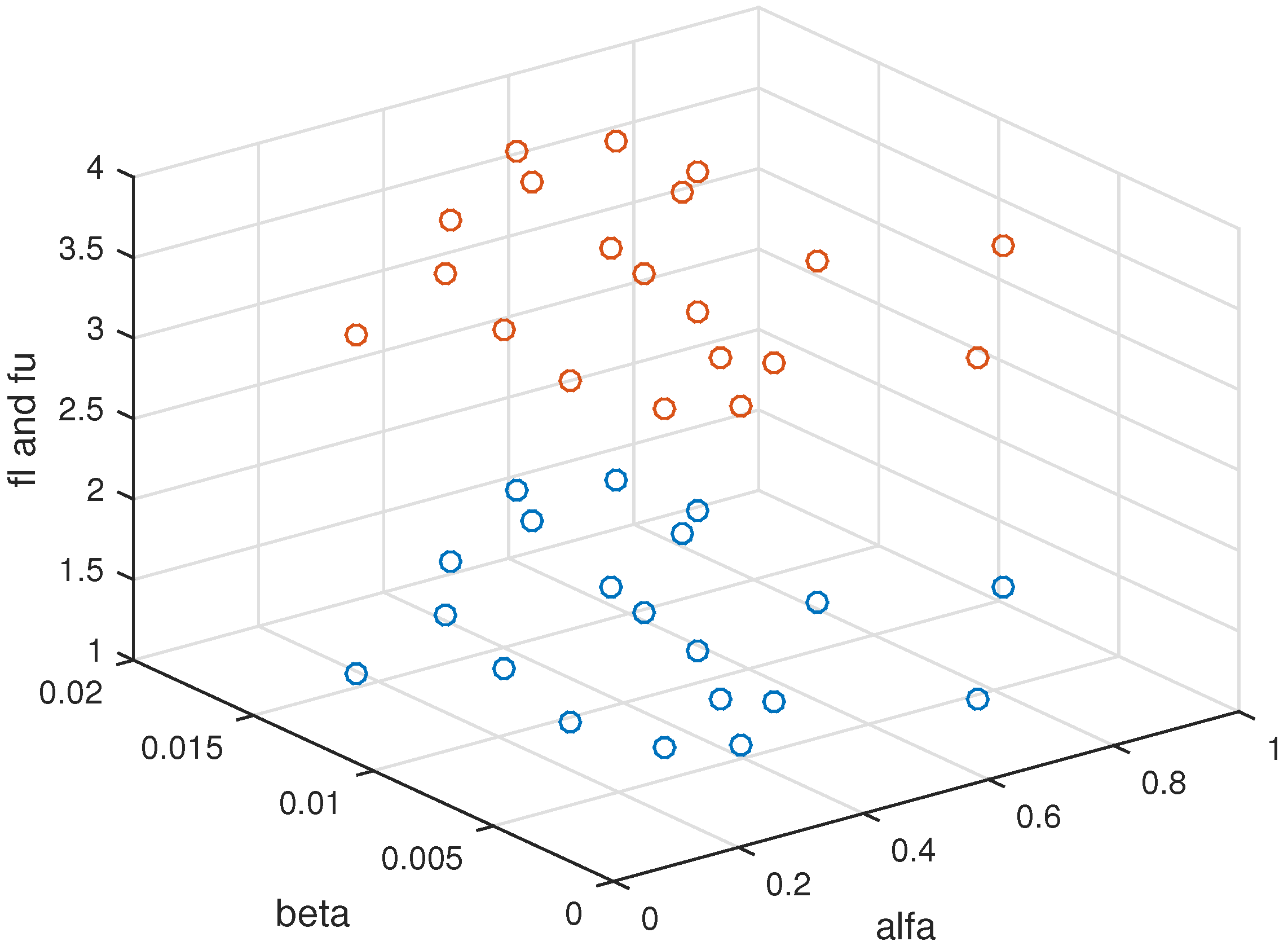
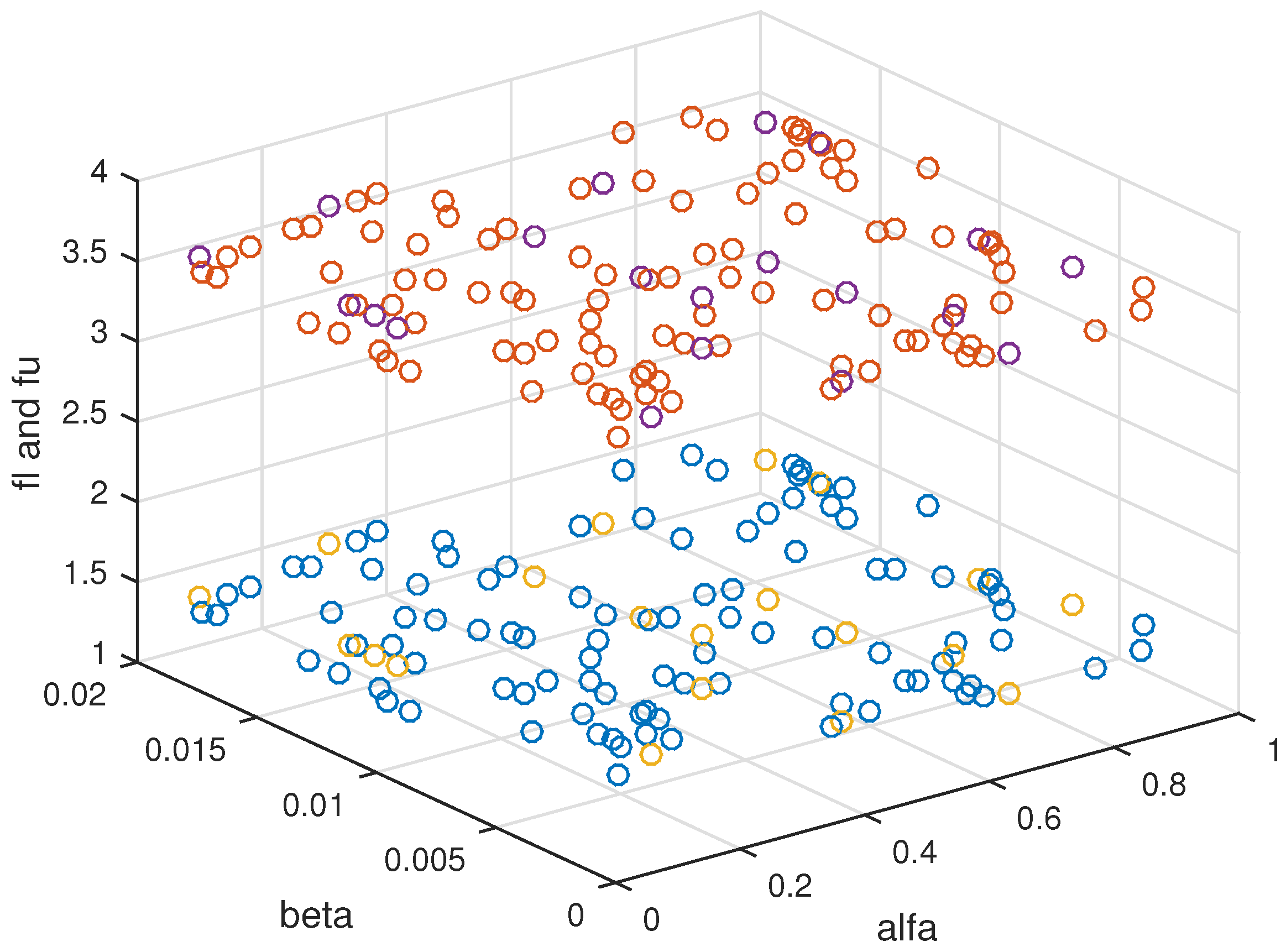
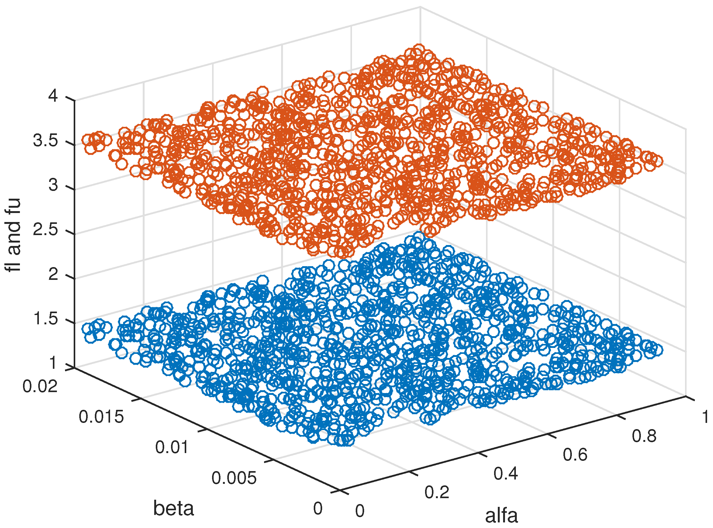
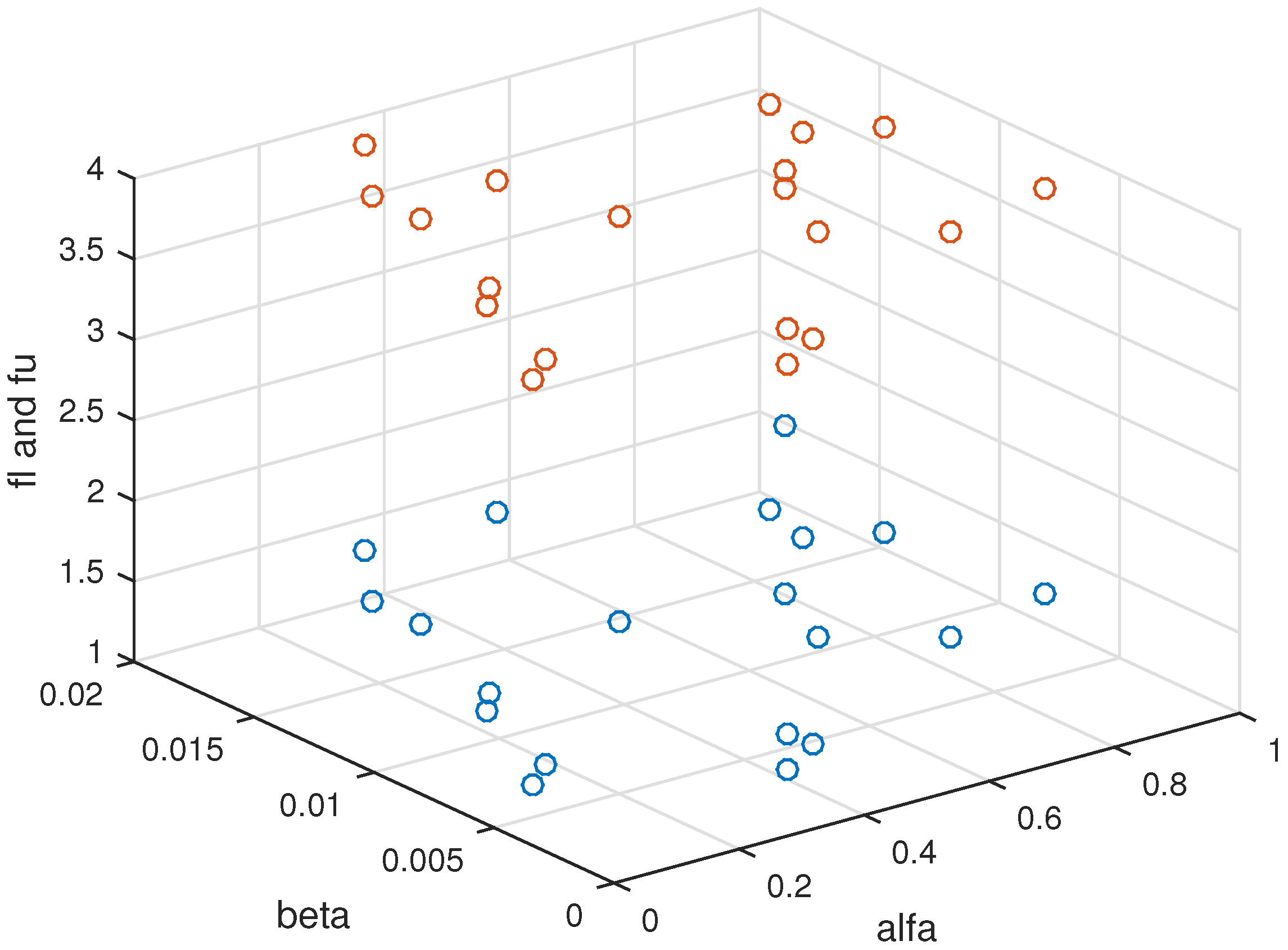
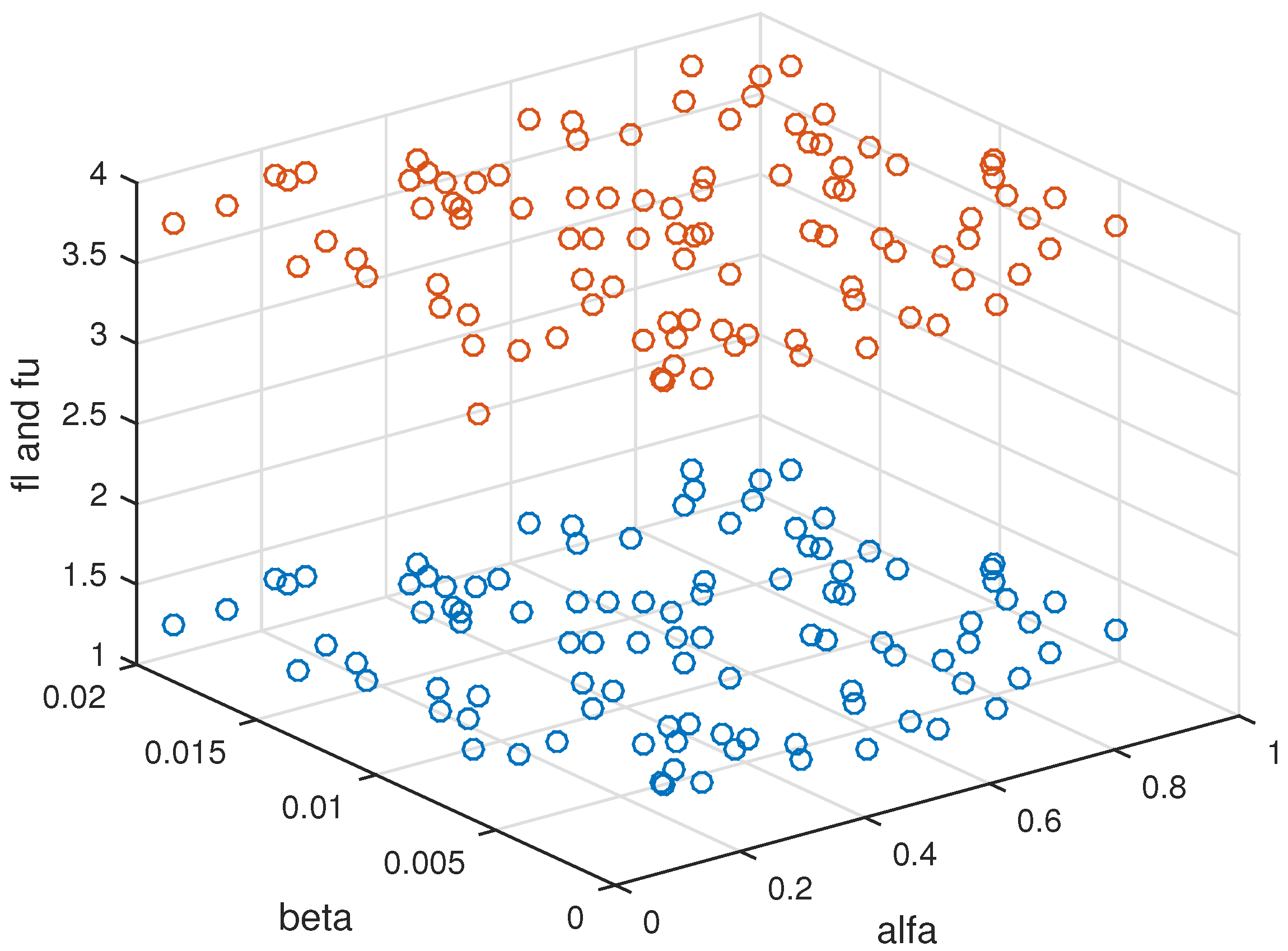
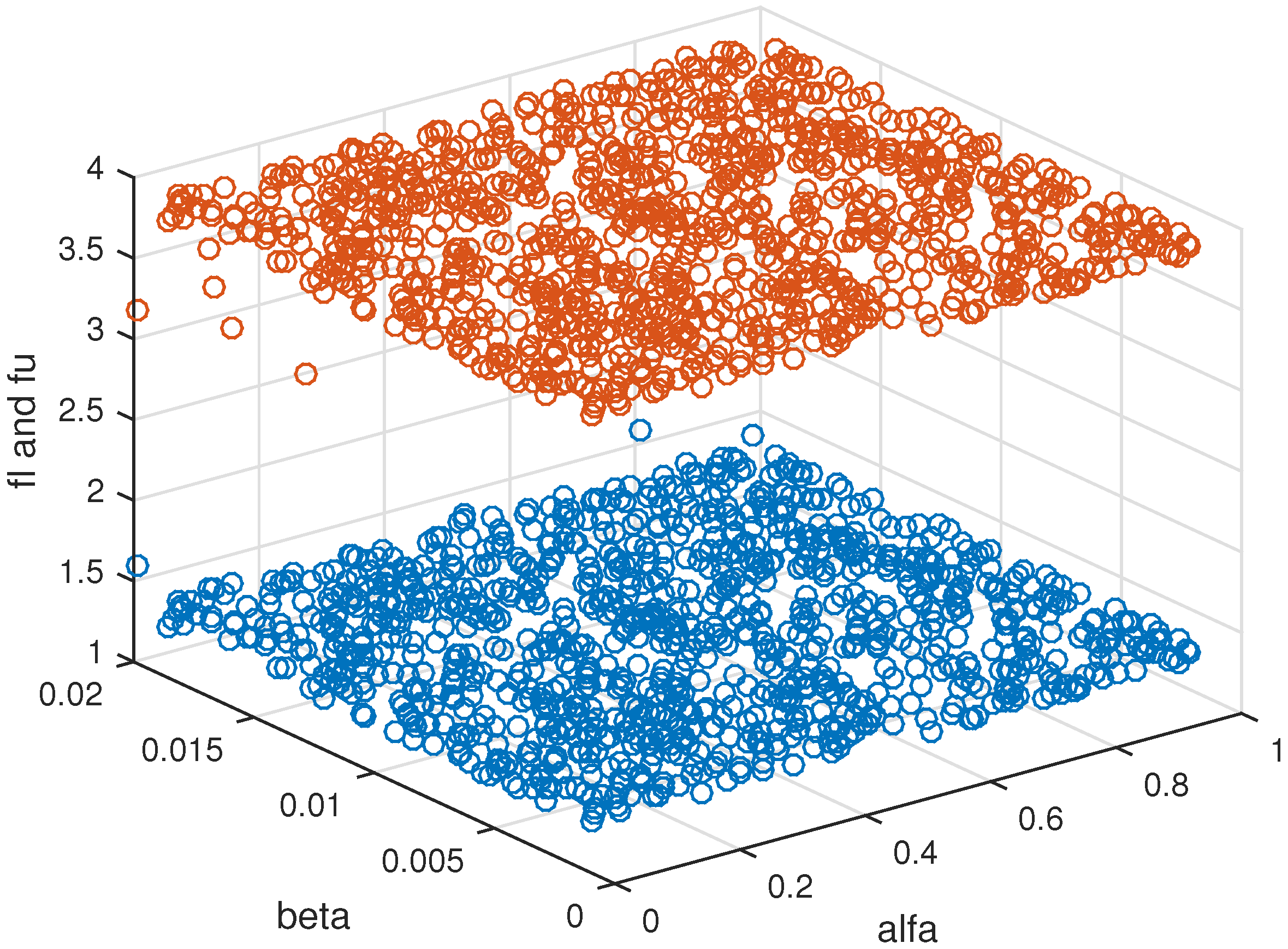
We present computational results on Examples 1 and 2 to compare the results due to Theorems 2 and 3. To compare the obtained results for the numerical examples, we use different diagrams and tables to show the advantages of the given Theorems 2 and 3 by showing that any solution of the problem or is an efficient solution of the problem . In addition, the efficient space for different pairs of is also shown, with the generated nonzero elements taken randomly in the interval and elements of vector given in with step length 1.
Example 1.
Consider the interval programming problem with SOC constraint as follows:
Example 2.
Consider the interval programming problem with SOC constraint as follows:
Example 3.
Consider the interval programming problem with SOC constraint as follows:
By our described methodology, we get a properly efficient solution. Here, and
For some the corresponding problem becomes:
This problem is an SOCP problem and can be solved by an interior point method.
If then the properly efficient solution is and the optimal interval is and efficient solution obtained by Theorem 2 is .
Table 2 shows the objective function values obtained using Theorems 2 and 3.
6. Conclusions
A very important concept of SOCP is investigated here. We have paid our attention to consider the interval fractional programming problem with second order cone constraints. To solve such problems, we established two important results concerning the efficient and properly efficient solutions of the second-order cone constrained interval programming problems. In addition and furthermore, a new notion of efficiency called efficient space was proposed due to interval form of the objective function and the corresponding obtained results were summarized in Table 3 and Table 4 and simultaneously in Figure 1, Figure 2, Figure 3, Figure 4, Figure 5 and Figure 6 with efficient spaces related to upper and lower bound properties of the interval problem. To illustrate the performance of our methodology, a few numerical examples were worked through to represent the importance of the study. The numerical results showed that the CPU times needed for solving problems with second order cone constraints are less than the ones for the problem without second-order cone constraints, which is a very important issue.
Author Contributions
A.S., M.S. and N.M.A. contributed to the design and implementation of the research, to the analysis of the results and to the writing of the manuscript.
Funding
This research received no external funding.
Acknowledgments
The authors are thankful to the Shahid Chamran University of Ahvaz and Sharif University of Technology for making this joint work possible and Shahid Chamran University of Ahvaz for the financial support.
Conflicts of Interest
The authors declare no conflict of interest.
References
- Bhurjee, A.K.; Panda, G. Efficient solution of interval optimization problem. Math. Meth. Oper. Res. 2012, 76, 273–288. [Google Scholar] [CrossRef]
- Moore, R.E. Interval Analysis; Prentice-Hall: Upper Saddle River, NJ, USA, 1966. [Google Scholar]
- Walster, G.W.; Hansen, E. Global Optimization Using Interval Analysis; Marcel Dekker, Inc.: New York, NY, USA, 2004. [Google Scholar]
- Wu, H. On interval-valued nonlinear programming problems. J. Math. Anal. Appl. 2008, 338, 299–316. [Google Scholar] [CrossRef]
- Charnes, A.; Cooper, W.W. Programs with linear fractional functions. Nav. Res. Logist. Q. 1962, 9, 181–196. [Google Scholar] [CrossRef]
- Tantawy, S.F. A new procedure for solving linear fractional programming problems. J. Math. Comput. Model. 2008, 48, 969–973. [Google Scholar] [CrossRef]
- Dinkelbach, W. On nonlinear fractional programming. Manag. Sci. 1967, 13, 492–498. [Google Scholar] [CrossRef]
- Alizadeh, F.; Goldfarb, D. Second-order cone programming. Math. Program. Ser. B 2003, 95, 35–51. [Google Scholar] [CrossRef]
- Lobo, M.S.; Vandenberghe, L.; Boyd, L.; Lebret, H. Applications of second order cone programming. Linear Algebra Appl. 1998, 284, 193–228. [Google Scholar] [CrossRef]
- Nesterov, Y.; Nemirovski, A. Interior Point Polynomial Methods in Convex Programming: Theory and Applications; Society for Industrial and Applied Mathematics (SIAM): Philadelphia, PA, USA, 1994. [Google Scholar]
- Lobo, M.S.; Vandenberghe, L.; Boyd, S. SOCP: Software for Second-Order Cone Programming; Information Systems Laboratory, Stanford University: Standford, CA, USA, 1997. [Google Scholar]
- Nesterov, Y.E.; Todd, M.J. Primal-dual interior-point methods for self-scaled cones. SIAM J. Optim. 1998, 8, 324–364. [Google Scholar] [CrossRef]
- Nesterov, Y.E.; Todd, M.J. Self-scaled barriers and interior-point methods for convex programming. Math. Oper. Res. 1997, 22, 1–42. [Google Scholar] [CrossRef]
- Kim, S.; Kojima, M. Exact solutions of some nonconvex quadratic optimization problems via SDP and SOCP relaxations. Comput. Optim. Appl. 2003, 26, 143–154. [Google Scholar] [CrossRef]
Figure 1.
Efficient space for Example 3 with SOC constraint using .

Figure 2.
Efficient space for Example 3 with SOC constraint using .

Figure 3.
Efficient space for Example 3 with SOC constraint using .

Figure 4.
Efficient space for Example 3 without SOC constraint using .

Figure 5.
Efficient space for Example 3 without SOC constraint using .

Figure 6.
Efficient space for Example 3 without SOC constraint using .


Table 1.
Notations.
| n | Number of pairs corresponding to and related to Theorem 3 |
| Exwsoc1 | Example 1 without SOC constraint |
| Exsoc1 | Example 1 with SOC constraint |
| Exwsoc2 | Example 2 without SOC constraint |
| Exsoc2 | Example 2 with SOC constraint |
| CPU | CPU time in seconds |
| CPU.ratio | The ratio of CPU times consumed by problem due to SOC constraint over without SOC constraint |
Table 2.
Objective function values using Theorems 2 and 3.
| Applying Theorem 2 | Applying Theorem 3 | |
|---|---|---|
| Example 1 | −12 | −0.003973 |
| Example 2 | 4.0454 | 171.31 |
Table 3.
CPU times corresponding to Example 1.
| n | CPU Time for Exwsoc1 | CPU Time for Exsoc1 | cpu.ratio |
|---|---|---|---|
| 10 | 0.764 | 1.2762 | |
| 50 | 4.013 | 2.760 | 1.454 |
| 100 | 7.353 | 5.320 | 1.3821 |
| 150 | 11.079 | 8.137 | 1.36155 |
| 200 | 14.674 | 10.543 | 1.392 |
| 250 | 18.435 | 12.890 | 1.43018 |
| 300 | 21.828 | 15.439 | 1.413822 |
| 350 | 25.269 | 18.388 | 1.37421 |
| 400 | 28.601 | 20.714 | 1.38076 |
| 450 | 32.044 | 22.860 | 1.40174 |
| 500 | 36.385 | 25.750 | 1.413 |
| 600 | 42.514 | 30.776 | 1.38140 |
| 700 | 49.899 | 35.852 | 1.39180 |
| 800 | 56.713 | 40.976 | 1.38405 |
| 900 | 64.219 | 45.873 | 1.39993 |
| 1000 | 71.645 | 51.256 | 1.398 |
Table 4.
CPU times corresponding to Example 2.
| n | CPU Time for Exwsoc2 | CPU Time for Exsoc2 | cpu.ratio |
|---|---|---|---|
| 10 | 1.621 | 1.225 | 1.32327 |
| 50 | 5.076 | 4.814 | 1.05442 |
| 100 | 9.608 | 9.154 | 1.0496 |
| 150 | 14.424 | 13.018 | 1.10800 |
| 200 | 18.695 | 17.185 | 1.02804 |
| 250 | 22.747 | 21.714 | 1.04752 |
| 300 | 26.842 | 25.866 | 1.03773 |
| 350 | 32.512 | 31.570 | 1.02983 |
| 400 | 36.399 | 33.455 | 1.0880 |
| 450 | 40.249 | 38.412 | 1.04782 |
| 500 | 45.471 | 42.775 | 1. 06303 |
| 600 | 54.623 | 52.015 | 1.05014 |
| 700 | 62.414 | 59.653 | 1.04628 |
| 800 | 71.676 | 68.400 | 1.04790 |
| 900 | 79.980 | 79.956 | 1.00030 |
| 1000 | 90.243 | 82.616 | 1.09231 |
© 2018 by the authors. Licensee MDPI, Basel, Switzerland. This article is an open access article distributed under the terms and conditions of the Creative Commons Attribution (CC BY) license (http://creativecommons.org/licenses/by/4.0/).
Share and Cite
MDPI and ACS Style
Sadeghi, A.; Saraj, M.; Mahdavi Amiri, N. Efficient Solutions of Interval Programming Problems with Inexact Parameters and Second Order Cone Constraints. Mathematics 2018, 6, 270. https://0-doi-org.brum.beds.ac.uk/10.3390/math6110270
AMA Style
Sadeghi A, Saraj M, Mahdavi Amiri N. Efficient Solutions of Interval Programming Problems with Inexact Parameters and Second Order Cone Constraints. Mathematics. 2018; 6(11):270. https://0-doi-org.brum.beds.ac.uk/10.3390/math6110270
Chicago/Turabian StyleSadeghi, Ali, Mansour Saraj, and Nezam Mahdavi Amiri. 2018. "Efficient Solutions of Interval Programming Problems with Inexact Parameters and Second Order Cone Constraints" Mathematics 6, no. 11: 270. https://0-doi-org.brum.beds.ac.uk/10.3390/math6110270
Note that from the first issue of 2016, this journal uses article numbers instead of page numbers. See further details here.