A Novel FMEA Model Based on Rough BWM and Rough TOPSIS-AL for Risk Assessment

Abstract

Failure mode and effects analysis (FMEA) is a risk assessment method that effectively diagnoses a product’s potential failure modes. It is based on expert experience and investigation to determine the potential failure modes of the system or product to develop improvement strategies to reduce the risk of failures. However, the traditional FMEA has many shortcomings that were proposed by many studies. This study proposes a hybrid FMEA and multi-attribute decision-making (MADM) model to establish an evaluation framework, combining the rough best worst method (R-BWM) and rough technique for order preference by similarity to an ideal solution technique (R-TOPSIS) to determine the improvement order of failure modes. In addition, this study adds the concept of aspiration level to R-TOPSIS technology (called R-TOPSIS-AL), which not only optimizes the reliability of the TOPSIS calculation program, but also obtains more potential information. This study then demonstrates the effectiveness and robustness of the proposed model through a multinational audio equipment manufacturing company. The results show that the proposed model can overcome many shortcomings of traditional FMEA, and effectively assist decision-makers and research and development (R&D) departments in improving the reliability of products.

1. Introduction

The failure mode and effects analysis (FMEA) method is widely used in various industries and is a management strategy tool based on teamwork and risk prevention in advance [1,2,3,4]. The FMEA technology is an active protection against failures that may occur in the future. “Prevention is better than treatment” is the spirit of FMEA, which effectively reduces maintenance costs and time. Three risk factors are defined in FMEA: the severity (S) caused by the failure, the probability of the occurrence (O) of the failure, and the detection (D) before the failure. The failure mode risk assessment is based on these three risk factors, with an assessment score ranging from one (lowest risk level) to 10 (highest risk level). These three evaluation scores are multiplied to obtain a risk priority number (RPN) with a minimum RPN of one and a maximum of 1000. Most studies using FMEA believe that there are many disadvantages to using RPN to judge the degree of risk, including the following:

(i)

The relative importance of the three risk factors (the weights of S, O, and D) is not considered [2,3,4,5];

(ii)

Different combinations of S, O, and D may form the same RPN, which does not mean that the meaning of risk is the same [2,3,4,5];

(iii)

The calculation through the multiplication of the three risk factors used by the RPN is too simplistic, and the evaluation model is not robust [1,2,3,4,5];

(iv)

The mathematical form of RPN is very sensitive to changes in risk factors [2,3,4,5];

(v)

There are other important risk factors not considered, such as expected cost (E) [3,5,6];

(vi)

The way in which the opinions of multiple experts are integrated is too simplistic and can easily lead to information loss [3].

There were many studies that incorporated FMEA into the multi-attribute decision-making (MADM) model to improve the applicability of risk assessment models and overcome these shortcomings and limitations [1,2,3,4,5,6,7]. This study proposes a novel model of FMEA based on MADM, which introduces rough set theory to the best worst method (BWM) and the technique for order preference by similarity to an ideal solution (TOPSIS) technique based on the aspiration level concept (R-BWM and R-TOPSIS-AL); both BWM and performance surveys are integrated using the rough number method to effectively retain expert opinions and add aspiration level to develop more practical improvement strategies and management implications [3,8]. The analysis procedure is divided into two phases. In the first phase, the FMEA decision-making team determines the risk factors and identifies the potential failure modes of the system or products. The risk factors developed by the traditional FMEA are retained in the study, including severity (S), occurrence (O), and detection (D). In addition, the expected cost (E) is added to reflect the financial budget constraints in practice [3,5,6]. Potential failure modes are determined based on expert experiences or historical error reporting of similar products. The second phase is the operational execution of R-BWM and R-TOPSIS-AL. BWM was proposed by Rezaei [9] to calculate the weights of criteria. BWM performs pairwise comparisons of the criteria in a structured manner. Compared to the analytic hierarchy process (AHP) method, BWM requires fewer pairs of comparisons and makes it easier to obtain good consistent results. This study uses R-BWM to generate a set of rough weights, confirming the relative importance of the four risk factors. In addition, R-TOPSIS-AL is used to determine the ranking of the failure modes. The ranking index used by R-TOPSIS-AL is based on Kuo [10], and many studies showed that this improved ranking index is highly reliable in practice [3,5,11].

The proposed model does not require any statistical assumptions, and the calculation process is rigorous and logical. An audio electronics manufacturing is used to demonstrate the usefulness and effectiveness of the proposed model. The proposed hybrid FMEA model makes some contributions and improvements to the manufacturing industry, including the following:

(i)

The risk factor of expected cost (E) is added to make the risk assessment system more complete;

(ii)

The expert opinions are integrated using the rough number method to improve the arithmetic mean to retain more expert information;

(iii)

The weights are calculated using the R-BWM method, and the number of pairwise comparisons of the contents of the questionnaire is greatly reduced, allowing more consistent results;

(iv)

For total assessment score of the failure modes, the R-TOPSIS-AL technique is used for its flexibility and reliability. It does not affect the speed of calculation and the quality of the solution because of the increase in the number of risk factors and failure modes;

(v)

The manufacturing industry can conduct a product risk analysis based on the proposed model, thereby reducing maintenance costs and troubleshooting time during development;

(vi)

The proposed model is not restricted to any industry, and various kinds of industries can use it to improve the quality, robustness, and life cycle of the product.

The rest of this article is organized as follows: Section 2 briefly reviews the FMEA and includes the development of the FMEA and the application of the MADM method in recent years. Section 3 describes the proposed FMEA model, including all the method reviews and detailed execution steps which are used and taken. Section 4 presents a real application case to demonstrate the feasibility and practicality of the proposed model. Section 5 describes management implications and conclusions, and describes future research.

2. A Brief Review of FMEA

FMEA is a system or product risk assessment method that was first proposed by the United States (US) military in 1940. This method was first used to evaluate the reliability of US military systems and military weapons, and finally officially published the military standard MIL-STD-1629 in 1949. However, the specification did not fully comply with the expectations and requirements of the US military and was, therefore, revised to MIL-STD-1629A in 1980 [12]. During the 1960s, the National Aeronautics and Space Administration (NASA) used FMEA in the Apollo space mission to effectively analyze the key factors that could fail in a space program. Furthermore, in 1985, the International Electrotechnical Commission (IEC) issued the International FMEA Standard (standard number: IEC 60812) and began applying FMEA to various industry risk assessments [13]. In 1993, the automotive industry used FMEA to assess possible risks in the product design phase and manufacturing process. The Automotive Industry Action Group (AIAG) and American Society for Quality (ASQ) worked with Daimler Chrysler Corporation, Ford Motor Company, and General Motors Corporation to develop a complete FMEA operating instruction manual to meet the quality system number QS-9000 requirements [14]. The International Organization for Standardization (ISO) is an international organization that sets specifications for quality standards. It uses FMEA as an important analytical tool for the production quality standard ISO 9000 series. Today, FMEA is used as a powerful technology for analyzing the safety and reliability of products and processes in a wide range of industries including the aerospace, nuclear, automotive, machinery, food, semiconductor, and pharmaceutical industries [3,4,15].

FMEA defines a set of criteria for evaluating typical risk factors, as shown in

Table 1. Three risk factor assessment scales for traditional failure mode and effects analysis (FMEA).

Level	Severity (S)	Occurrence (O)	Detection (D)
1	No	Almost never	Almost certain
2	Very slight	Remote	Very high
3	Slight	Very slight	High
4	Minor	Slight	Moderately high
5	Moderate	Low	Medium
6	Significant	Medium	Low
7	Major	Moderately high	Slight
8	Extreme	High	Very slight
9	Serious	Very high	Remote
10	Hazardous	Almost certain	Almost impossible

[16]. By calculating the RPN, engineers can immediately focus on improving the failure mode of the highest RPN, instead of focusing on all failure modes. Also, they can improve their priorities through assessments to prevent catastrophic risk incidents. The success of FMEA can significantly reduce system or product failure rates to improve the operational robustness of governments, businesses, and organizations.

With development, FMEA combined many different methods to optimize risk assessment models, with MADM being the most prominent. For example, Chemweno et al. [17] developed an FMEA-based risk assessment model for asset maintenance decisions that used the analytic network process (ANP) approach to consider the interdependence of risk factors. The risk factors chosen were based on the ISO 31000:2009 concept. Zhao et al. [18] used the Multiplicative form with Multi-Objective Optimization Ratio Analysis (MULTIMOORA) method combined with FMEA to establish a failure detection model. The model analyzed the failure factors of the steel plate process based on the RPN value. The study pointed out that the traditional RPN value does not consider the indirect relationship of risk factors with each other, which causes the analysis results to be inconsistent with the actual situation. Safari et al. [19] used Visekriterijumska Optimizacija i Kompromisno Resenje (VIKOR) technology to calculate the RPN value of the FMEA system, reducing the risk of business operations by improving key failure modes to facilitate the management performance of the organization.

Wang et al. [20] developed a fuzzy ambiguous FMEA model in which interval-valued intuitionistic fuzzy sets (IVIFs) were used to reflect the risk ambiguity of failure modes. The study used the hospital service process as a practical case to illustrate the accuracy, validity, and flexibility of the model. Ahn et al. [21] introduced fuzzy logic to express the subjective and empirical uncertainty of experts. Their model provided a flexible way to draw a risk picture for a hybrid molten carbonate fuel cell and gas turbine system, which divided 35 components into 70 potential failure factors, identifying key failure factors via FMEA to enhance the product reliability. Fattahi and Khalilzadeh [22] used the development of a hybrid MADM combined with the FMEA model and the AHP method to obtain the relative weights of S, O, D, and failure modes, and applied the MULTIMOORA method to identify the key failure factors of a steel company. Zhou and Thai [23] proposed a hybrid model based on fuzzy and gray theory to predict the failures of tanker equipment. They not only reduce the likelihood of equipment failures, but also improve the robustness of the tanker system. Mohsen and Fereshteh [7] proposed that the D number integrates the uncertainty of multiple experts in the judgment process. The study showed that FMEA is headed toward how to integrate multiple expert opinions. Lo et al. [3] proposed R-BWM in combination with R-TOSPSIS to determine the improvement order of failure modes for machine tools. This paper extends the methodology of their research, adding the concept of aspiration level to optimize the computational process, which can provide more persuasive improvements to meet the actual situation of all walks of life.

3. The Proposed FMEA Model Based on R-BWM and R-TOPSIS-AL

This section firstly introduces the rough number method, which integrates information from multiple experts. Subsequently, the R-BWM method is introduced to obtain the risk factor weighing procedure, which not only reduces the number of pairs of comparisons, but also obtains more consistent results. Finally, the concept of R-TOPSIS technology combined with the aspiration level (R-TOPSIS-AL) and its calculation steps are explained.

3.1. Rough Number

MADM issues are usually assessed by multiple experts. In the process of group decision-making, an effective method for integrating expert opinions and judgments is needed. Most of the research uses data considered to be an average or simple weighing method to integrate multiple experts. The computational concept of the rough number method is derived from the rough set theory [24], which is used to construct the upper and lower approximations of the decision-making group information. The main process consists of the following three steps:

Step 1. Determine Lower and Upper Approximations of Rough Numbers

Suppose we have an information system $S=\left(U,A\right)$, $E\subseteq U\left(E=\left\{e_1,e_2,\dots ,e_v\right\}\right)$, and $Apr\subseteq A$. Our task is to describe the set E based on the attribute values of Apr. For this, we define two operations, assigning to every $e_v\subseteq U$ two sets $\underset{\_}{Apr}\left(E\right)$ and $\overline{Apr}\left(E\right)$, called the lower and upper approximations of e_v, respectively, defined as follows:

Lower approximation:

$$\underset{\_}{Apr}\left(E\right)={\cup }_{e_v\in U}Apr\left(e_v\right):Apr\left(e_v\right)\subseteq E.$$

(1)

Upper approximation:

$$\overline{Apr}\left(E\right)={\cup }_{e_v\in U}Apr\left(e_v\right):Apr\left(e_v\right)\cap E\ne 0.$$

(2)

Step 2. Obtain Lower and Upper Limits of Rough Numbers

A group of expert judgments can be presented using rough lower and upper limits $\left(\underset{\_}{Lim}\left(e_v\right),\overline{Lim}\left(e_v\right)\right)$, which are calculated using the mean of the elements in the lower and upper approximations, respectively.

$$\underset{\_}{Lim}\left(e_v\right)=\frac{{\displaystyle {\sum }_{i=1}^{N_L}}{a}_i}{N_L},$$

(3)

$$\overline{Lim}\left(e_v\right)=\frac{{\displaystyle {\sum }_{i=1}^{N_U}}{b}_i}{N_U},$$

(4)

where a_i and b_i are the elements in the lower and upper approximations of e_v, respectively. In addition, N_L and N_U represent the total number of objects involved in the lower and upper approximations of e_v, respectively.

Step 3. Obtain Interval Value of Rough Numbers

Equations (3) and (4) can be used to convert the judgments of a group of experts into a set of rough numbers $RN\left(e_v\right)$, as shown in Equation (5).

$$RN\left(e_v\right)=\left[e_v^L,e_v^U\right]=\left[\underset{\_}{Lim}\left(e_v\right),\overline{Lim}\left(e_v\right)\right].$$

(5)

Furthermore, for two rough numbers $RN\left(\alpha \right)=\left[\underset{\_}{Lim}\left(\alpha \right),\overline{Lim}\left(\alpha \right)\right]$ and $RN\left(\beta \right)=\left[\underset{\_}{Lim}\left(\beta \right),\overline{Lim}\left(\beta \right)\right]$, arithmetic operations for rough numbers can be shown using Equations (6)–(10) as follows:

$$RN\left(\alpha \right)\times \delta =\left[\underset{\_}{Lim}\left(\alpha \right),\overline{Lim}\left(\alpha \right)\right]\times \delta =\left[\underset{\_}{Lim}\left(\alpha \right)\times \delta ,\overline{Lim}\left(\alpha \right)\times \delta \right],$$

(6)

$$RN\left(\alpha \right)+RN\left(\beta \right)\begin{array}{l}=\left[\underset{\_}{Lim}\left(\alpha \right),\overline{Lim}\left(\alpha \right)\right]+\left[\underset{\_}{Lim}\left(\beta \right),\overline{Lim}\left(\beta \right)\right]\\ =\left[\underset{\_}{Lim}\left(\alpha \right)+\underset{\_}{Lim}\left(\beta \right),\overline{Lim}\left(\alpha \right)+\overline{Lim}\left(\beta \right)\right]\end{array}$$

(7)

$$RN\left(\alpha \right)-RN\left(\beta \right)\begin{array}{l}=\left[\underset{\_}{Lim}\left(\alpha \right),\overline{Lim}\left(\alpha \right)\right]-\left[\underset{\_}{Lim}\left(\beta \right),\overline{Lim}\left(\beta \right)\right]\\ =\left[\underset{\_}{Lim}\left(\alpha \right)-\overline{Lim}\left(\beta \right),\overline{Lim}\left(\alpha \right)-\underset{\_}{Lim}\left(\beta \right)\right]\end{array}$$

(8)

$$RN\left(\alpha \right)\times RN\left(\beta \right)\begin{array}{l}=\left[\underset{\_}{Lim}\left(\alpha \right),\overline{Lim}\left(\alpha \right)\right]\times \left[\underset{\_}{Lim}\left(\beta \right),\overline{Lim}\left(\beta \right)\right]\\ =\left[\underset{\_}{Lim}\left(\alpha \right)\times \underset{\_}{Lim}\left(\beta \right),\overline{Lim}\left(\alpha \right)\times \overline{Lim}\left(\beta \right)\right]\end{array}$$

(9)

$$RN\left(\alpha \right)/RN\left(\beta \right)\begin{array}{l}=\left[\underset{\_}{Lim}\left(\alpha \right),\overline{Lim}\left(\alpha \right)\right]-\left[\underset{\_}{Lim}\left(\beta \right),\overline{Lim}\left(\beta \right)\right]\\ =\left[\underset{\_}{Lim}\left(\alpha \right)/\overline{Lim}\left(\beta \right),\overline{Lim}\left(\alpha \right)/\underset{\_}{Lim}\left(\beta \right)\right]\end{array}$$

(10)

where $\delta$ is a nonzero constant.

A simple example is used to detail the calculation of the rough numbers. Suppose four experts evaluate the evaluation values of an object A as 4, 4, 3, and 2, respectively, and the following rough numbers can be obtained with the use of Equations (1)–(5):

$$\begin{array}{l}\underset{\_}{Lim}\left(4\right)=\left(2+3+4+4\right)/4=3.25,\overline{Lim}\left(4\right)=\left(4+4\right)/2=4\\ \Rightarrow RN\left(A^{\left(1\right)}\right)=RN\left(A^{\left(2\right)}\right)=RN\left(4\right)=\left[3.25,4\right]\\ \underset{\_}{Lim}\left(3\right)=\left(2+3\right)/2=2.5,\overline{Lim}\left(3\right)=\left(3+4+4\right)/3=3.667\\ \Rightarrow RN\left(A^{\left(3\right)}\right)=RN\left(3\right)=\left[2.5,3.667\right]\\ \underset{\_}{Lim}\left(2\right)=2,\overline{Lim}\left(2\right)=\left(2+3+4+4\right)/4=3.25\Rightarrow RN\left(A^{\left(4\right)}\right)=RN\left(2\right)=\left[2,3.25\right].\end{array}$$

This set of scores can be obtained by averaging as follows:

$$RN\left(A\right)=\left[\left(3.25+3.25+2.5+2\right)/4,\left(4+4+3.667+3.25\right)/4\right]=\left[2.750,3.729\right].$$

3.2. Rough Best Worst Method

The advantage of BWM is that it provides a more accurate set of information with a simpler questionnaire to obtain a unique set of best weights $w_j^{*}$ [9]. In the established evaluation framework, the expert k is required to use a scale of 1–9 for a pairwise comparison of the j criteria, where k = 1, 2, …, p; j = 1, 2, …, n. In the FMEA question, the evaluation criteria refer to the risk factor. Experts k provide ratings based on their professional experience. Therefore, the initial pairwise comparison matrix of expert k can be defined as follows:

$$X^{\left(k\right)}=\left[\begin{array}{cccc}1& x_{12}^{\left(k\right)}& \cdots & x_{1n}^{\left(k\right)}\\ \raisebox{1ex}{$1$}\!\left/ \!\raisebox{-1ex}{$x_{12}^{\left(k\right)}$}\right.& 1& \cdots & x_{2n}^{\left(k\right)}\\ ⋮& ⋮& \ddots & ⋮\\ \raisebox{1ex}{$1$}\!\left/ \!\raisebox{-1ex}{$x_{1n}^{\left(k\right)}$}\right.& \raisebox{1ex}{$1$}\!\left/ \!\raisebox{-1ex}{$x_{2n}^{\left(k\right)}$}\right.& \cdots & 1\end{array}\right],$$

(11)

where $x_{ij}^{\left(k\right)}$ indicates the relative importance of the factor i for the factor j evaluated by the expert k. The AHP method is a way of using this pairwise comparison. This matrix requires a pairwise comparison of n(n − 1)/2 times. However, BWM only needs 2n − 3 comparison times to determine a set of optimal weights and achieve better consistent results.

The application of BWM to solve various MADM problems shows practicality and effectiveness. There were some articles that used the approximate number combined with BWM to integrate expert opinions. Pamučar et al. [25] first proposed a method combining the rough number and BWM to evaluate the optimal location of a wind power plant in Serbia. In the same year, Stević et al. [26] proposed a hybrid model to select the best transport truck type for logistics companies. The model used R-BWM to calculate the weights of eight criteria and used rough simple additive weighting (SAW) to obtain the priority order of the eight alternatives. The study indicated that the developed model was effective for the application of selecting internal transport logistics trucks in the paper industry. In the following year, Stević et al. [27] combined R-BWM with rough weighted aggregated sum product assessment (WASPAS) to overcome the problem of the excessive sensitivity of rough SAW. They used this method for site selection of roundabout construction to support decision-makers in solving Doboj traffic congestion problems. Stević et al. [28] extended the method of R-BWM to the service industry and explored the service quality of international technology conferences based on the Service Quality (SERVQUAL) model. A total of 104 scholars participated in the discussion of the topic, and the results showed that R-BWM effectively integrated the opinions of many scholars and developed the best weights to illustrate the relative importance of the evaluation criteria. However, their R-BWM required experts to choose the same best and worst criteria. Our study uses the R-BWM method proposed by Lo et al. [3], which does not require that all experts choose the same best and worst criteria. This approach focuses on the integration of expert opinions. The detailed steps of R-BWM are as follows:

Step 1. Identify N Risk Factors

The experts establish a complete evaluation framework for the discussion of the topic, which identifies n factors $\left\{c_1,c_2,\dots ,c_n\right\}$.

Step 2. Determine the Best and Worst Risk Factors

Each expert considers the factors determined in Step 1, choosing the factors that have the best (most important) and worst (least important) impact on the topic. Since each expert has a different background, the chosen risk factors do not have to be the same. The impact of this step on the weight calculation results is the most critical.

Step 3. Get Best-to-Others and Others-to-Worst Vectors (BO and OW Vectors)

Each expert evaluates the relative importance $A_{Bj}^{\left(k\right)}$ of the best factor B to other factors j to get the best-to-others (BO) vector.

$$A_{Bj}^{\left(k\right)}=\left(a_{B1}^{\left(k\right)},a_{B2}^{\left(k\right)},\dots ,a_{Bn}^{\left(k\right)}\right).$$

Similarly, each expert evaluates the relative importance $A_{jW}^{\left(k\right)}$ of other factors j to the worst-case factor W to get the others-to-worst (OW) vector.

$$A_{jW}^{\left(k\right)}={\left(a_{1W}^{\left(k\right)},a_{2W}^{\left(k\right)},\dots ,a_{nW}^{\left(k\right)}\right)}^T.$$

The relative importance of self-to-self for each factor would be one since they are equally important, that is, $A_{BB}^{\left(k\right)}=1$ and $A_{WW}^{\left(k\right)}=1$.

Step 4. Use the Rough Number Method to Get Rough Best-to-Others and Rough Others-to-Worst Vectors (Rough BO and Rough OW Vectors)

The BO and OW vectors of all experts can be generated via Steps 1–3; then, the BO and OW vectors are integrated using the approximate number method, as shown in Equations (1)–(5). Note that only the information selected by experts with the same best and worst criteria can be integrated. The resulting rough BO and rough OW vectors are as follows

$$RN\left(A_{Bj}\right)=\left[{\underset{\_}{a}}_{Bj},{\overline{a}}_{Bj}\right]=\left(\left[{\underset{\_}{a}}_{B1},{\overline{a}}_{B1}\right],\left[{\underset{\_}{a}}_{B2},{\overline{a}}_{B2}\right],\dots ,\left[{\underset{\_}{a}}_{Bn},{\overline{a}}_{Bn}\right]\right);$$

(12)

$$RN\left(A_{jW}\right)=\left[{\underset{\_}{a}}_{jW},{\overline{a}}_{jW}\right]={\left(\left[{\underset{\_}{a}}_{1W},{\overline{a}}_{1W}\right],\left[{\underset{\_}{a}}_{2W},{\overline{a}}_{2W}\right],\dots ,\left[{\underset{\_}{a}}_{nW},{\overline{a}}_{nW}\right]\right)}^T.$$

(13)

Step 5. Calculate the Best Approximate Weights

After the rough optimal weights of the RPN elements are determined, the maximum absolute differences $\left|\frac{\left({\underset{\_}{w}}_B,{\overline{w}}_B\right)}{\left({\underset{\_}{w}}_j,{\overline{w}}_j\right)}-\left({\underset{\_}{a}}_{Bj},{\overline{a}}_{Bj}\right)\right|$ and $\left|\frac{\left({\underset{\_}{w}}_j,{\overline{w}}_j\right)}{\left({\underset{\_}{w}}_W,{\overline{w}}_W\right)}-\left({\underset{\_}{a}}_{jW},{\overline{a}}_{jW}\right)\right|$ of all j are minimized, which can be converted into the following linear programming equation:

$$\begin{array}{l}\min {\xi }^{*}\\ s.t.\{\begin{array}{l}\left|\frac{\left({\underset{\_}{w}}_B,{\overline{w}}_B\right)}{\left({\underset{\_}{w}}_j,{\overline{w}}_j\right)}-\left({\underset{\_}{a}}_{Bj},{\overline{a}}_{Bj}\right)\right|\le {\xi }^{*};\\ \left|\frac{\left({\underset{\_}{w}}_j,{\overline{w}}_j\right)}{\left({\underset{\_}{w}}_W,{\overline{w}}_W\right)}-\left({\underset{\_}{a}}_{jW},{\overline{a}}_{jW}\right)\right|\le {\xi }^{*};\\ {\displaystyle \sum _{j=1}^n\left(\frac{{\underset{\_}{w}}_j^{*}+{\overline{w}}_j^{*}}{2}\right)=1;}\\ {\overline{w}}_j^{*}\ge {\underset{\_}{w}}_j^{*}\ge 0,\mathrm{for}\mathrm{all}j.\end{array}\end{array}$$

(14)

By multiplying the denominator and disassembling the absolute value, the linear programming equation is converted to

$$\begin{array}{l}\min {\xi }^{*}\\ s.t.\{\begin{array}{l}{\underset{\_}{w}}_B-{\underset{\_}{a}}_{Bj}\cdot {\overline{w}}_j\le {\xi }^{*}\cdot {\overline{w}}_j;\\ {\underset{\_}{w}}_B-{\underset{\_}{a}}_{Bj}\cdot {\overline{w}}_j\ge -{\xi }^{*}\cdot {\overline{w}}_j;\\ {\overline{w}}_B-{\overline{a}}_{Bj}\cdot {\underset{\_}{w}}_j\le {\xi }^{*}\cdot {\underset{\_}{w}}_j;\\ {\overline{w}}_B-{\overline{a}}_{Bj}\cdot {\underset{\_}{w}}_j\ge -{\xi }^{*}\cdot {\underset{\_}{w}}_j;\\ {\underset{\_}{w}}_j-{\underset{\_}{a}}_{jW}\cdot {\overline{w}}_W\le {\xi }^{*}\cdot {\overline{w}}_W;\\ {\underset{\_}{w}}_j-{\underset{\_}{a}}_{jW}\cdot {\overline{w}}_W\ge -{\xi }^{*}\cdot {\overline{w}}_W;\\ {\overline{w}}_j-{\overline{a}}_{jW}\cdot {\underset{\_}{w}}_W\le {\xi }^{*}\cdot {\underset{\_}{w}}_W;\\ {\overline{w}}_j-{\overline{a}}_{jW}\cdot {\underset{\_}{w}}_W\ge -{\xi }^{*}\cdot {\underset{\_}{w}}_W;\\ {\displaystyle \sum _{j=1}^n\left(\frac{{\underset{\_}{w}}_j^{*}+{\overline{w}}_j^{*}}{2}\right)=1;}\\ {\overline{w}}_j^{*}\ge {\underset{\_}{w}}_j^{*}\ge 0,\mathrm{for}\mathrm{all}j.\end{array}\end{array}$$

(15)

In this study, the approximate upper and lower limits are equally important. After the linear programming problem is solved, the approximate optimal weight $RN\left(w_j^{*}\right)=\left(\left[{\underset{\_}{w}}_1^{*},{\overline{w}}_1^{*}\right],\left[{\underset{\_}{w}}_2^{*},{\overline{w}}_2^{*}\right],\dots ,\left[{\underset{\_}{w}}_n^{*},{\overline{w}}_n^{*}\right]\right)$, and the best value of $\xi$, which is represented by ${\xi }^{*}$, can be obtained. ${\xi }^{*}$ is defined as the consistency ratio (CR) of the overall pairwise comparison system. When the best and worst risk factors selected by the experts are different, they can be divided into r groups, and each group generates a set of approximate weights. The final best approximate weight can be integrated by the ratio of each group of people to the total number of people assessed (represented by ${\Omega }_i$).

$$RN\left(w_j^{*}\right)={\Omega }_1\cdot RN{\left(w_j\right)}^{\left(G1\right)}+{\Omega }_2\cdot RN{\left(w_j\right)}^{\left(G2\right)}+\cdots +\left(1-{\displaystyle \sum _{i=1}^{r-1}{\Omega }_i}\right)\cdot RN{\left(w_j\right)}^{\left(Gr\right)};$$

(16)

$$RN\left(w_j^{*}\right)={\displaystyle \sum _{i=1}^r\left({\Omega }_i\cdot RN{\left(w_j\right)}^{\left(G_i\right)}\right)}.$$

(17)

3.3. Rough Modified TOPSIS-AL

TOPSIS technology is one of the most popular MADM methods for performance value integration and alternative sequencing. The method finds positive and negative ideal solutions (PIS and NIS) in the alternative combination and determines the relative position of each alternative by calculating the distances from each alternative to PIS and NIS. The best alternative is the one closest to PIS and farthest from NIS. In this paper, the alternative is the failure mode. TOPSIS technology is easy to operate and understand and was used for many problems [3,10]. The R-TOPSIS technique was proposed by Lo et al. [3] to represent the consensus of multiple experts in the form of approximate intervals. This study introduces the concept of aspiration level into R-TOPSIS, called R-TOPSIS-AL. A relatively good solution from the existing alternatives is replaced by aspiration levels fitting today’s competitive markets. Therefore, the original R-TOPSIS method is modified to define the aspiration level as the PIS, and the worst value as the NIS; therefore, “picking the best apple from a bucket of rotten apples” can be avoided. Also, we used the study by Kuo [10] to develop a new TOPSIS ranking index that considers not only the distances from all alternatives to PIS and NIS, but also the weights of these two distances. The R-TOPSIS-AL technical calculation procedure is as follows:

Step 1. Obtain the Initial Evaluation Matrix

Suppose the FMEA team has k experts, j risk factors, and i failure modes, where k = 1, 2, …, p; j = 1, 2, …, n; and i = 1, 2, …, m. Then, the initial evaluation matrix is as follows:

$$Y^{(k)}=\left[\begin{array}{cccc}{y}_{11}^{(k)}& y_{12}^{(k)}& \cdots & y_{1n}^{(k)}\\ y_{21}^{(k)}& y_{22}^{(k)}& \cdots & y_{2n}^{(k)}\\ ⋮& ⋮& \ddots & ⋮\\ y_{m1}^{(k)}& y_{m2}^{(k)}& \cdots & y_{mn}^{(k)}\end{array}\right],$$

(18)

where $y_{ij}^{(k)}$ indicates the evaluation value of the i failure mode under the j risk factor evaluated by the expert k.

Step 2. Calculate the Approximate Initial Matrix

Use the rough number method to convert multiple expert evaluation values into approximate initial matrices, as follows:

$$RN\left(Y\right)=\left[\begin{array}{cccc}RN\left(y_{11}\right)& RN\left(y_{12}\right)& \cdots & RN\left(y_{1n}\right)\\ RN\left(y_{21}\right)& RN\left(y_{22}\right)& \cdots & RN\left(y_{2n}\right)\\ ⋮& ⋮& \ddots & ⋮\\ RN\left(y_{m1}\right)& RN\left(y_{m2}\right)& \cdots & RN\left(y_{mn}\right)\end{array}\right],$$

(19)

where $RN\left(y_{ij}\right)$ represents a set of approximate numbers $\left[{\underset{\_}{y}}_{ij},{\overline{y}}_{ij}\right]$.

Step 3. Get the Normalized Approximate Matrix

The purpose of normalization is to unify the evaluation units of all risk factors and to convert the evaluation values to a range of 0–1. The traditional normalization method is to use the current evaluation maximum as the denominator, shown as follows:

$$RN\left(Y^{*}\right)=\left[\frac{{\underset{\_}{y}}_{ij}}{{\max }_j\left\{{\overline{y}}_{ij}\right\}},\frac{{\overline{y}}_{ij}}{{\max }_j\left\{{\overline{y}}_{ij}\right\}}\right].$$

(20)

However, this approach is equivalent to choosing a better apple among a barrel of rotten apples. According to the concept of aspiration level proposed by Liou [8], we increased the aspiration and tolerable level in the failure mode. In this study, the aspiration level is seen as the denominator of normalization. Therefore, after R-TOPSIS-AL analysis, the gap between each failure mode and the aspiration level can be clearly understood, and the improvement strategy can be further determined. The normalized approximate matrix is expressed as follows:

$$RN\left(Y^{*}\right)=\left[\frac{{\underset{\_}{y}}_{ij}}{y^{*}},\frac{{\overline{y}}_{ij}}{y^{*}}\right],$$

(21)

where $y^{*}$ is the aspiration level of the evaluation system, and $y^{*}=10$.

Step 4. Obtain a Weighted Normalized Approximate Matrix

We consider the relative importance of the risk factors, thereby multiplying the calculated weights of R-BWM by the normalized approximate matrix to obtain the weighted normalization matrix, which is expressed as follows:

$$RN\left(Y^{**}\right)=RN\left(w_j{}^{*}\right)\cdot RN\left(Y^{*}\right).$$

(22)

Step 5. Determine PIS and NIS

Based on the concept of aspiration level, PIS and NIS should be 1 and 0.1 after normalization. Therefore, after considering the weights, the PIS and NIS of the system can be obtained as shown below.

$$\mathrm{PIS}=\left(r_1^{+},r_2^{+},\dots ,r_n^{+}\right)=\left(1\cdot w_1^{*},1\cdot w_2^{*},\dots ,1\cdot w_n^{*}\right);$$

(23)

$$\mathrm{NIS}=\left(r_1^{-},r_2^{-},\dots ,r_n^{-}\right)=\left(0.1\cdot w_1^{*},0.1\cdot w_2^{*},\dots ,0.1\cdot w_n^{*}\right).$$

(24)

Step 6. Calculate the Separation Distance of Each Failure Mode to the PIS and NIS

The Euclidean distances are used to define how well failure mode i is separated from PIS and NIS. The R-TOPSIS-AL proposed in this paper does not require a de-rough procedure to obtain a crisp value. In this step, considering that the approximate upper bound and the lower bound are equally important, the process of converting to a crisp value is through dividing them by two, which is expressed as follows:

$$d_i^{+}={\displaystyle \sum _{j=1}^n\sqrt{\left(\frac{{\left(r_j^{+}-{\underset{\_}{r}}_{ij}\right)}^2+{\left(r_j^{+}-{\overline{r}}_{ij}\right)}^2}{2}\right)}},i=1,2,\dots ,m$$

(25)

$$d_i^{-}={\displaystyle \sum _{j=1}^n\sqrt{\left(\frac{{\left({\underset{\_}{r}}_{ij}-r_j^{-}\right)}^2+{\left({\overline{r}}_{ij}-r_j^{-}\right)}^2}{2}\right)}},i=1,2,\dots ,m$$

(26)

Step 7. Calculate the Closeness Coefficient

The new closeness coefficient (CC_i) was proposed by Kuo [10] and is a reliable calculation method. The ranking index has a very good basis for judgment because the sum of CC_i is equal to zero. The value of CC_i ranges from −1 to 1, and a more positive CC_i means that it is closer to the aspiration level. Conversely, a more negative CC_i means that it is closer to the worst value.

$$C{C}_h=w^{+}\left(d_h^{-}/{\displaystyle \sum _{h=1}^m{d}_h^{-}}\right)-w^{-}\left(d_h^{*}/{\displaystyle \sum _{h=1}^m{d}_h^{*}}\right),\{\begin{array}{l}-1\le C{C}_h\le 1,h=1,2,\dots ,m\\ 0\le w^{+}\le 1\\ 0\le w^{-}\le 1\end{array},$$

(27)

where w⁺ and w⁻ respectively represent the weights reflecting the relative importance of PIS and NIS in the decision-maker’s consciousness. When the decision-maker believes that the distance from the PIS is important, w⁻ is set to be greater than 0.5. Since w⁺ + w⁻ = 1, the settings of w⁺ and w⁻ affect each other. In general, w⁺ and w⁻ are both set to 0.5 when there are no special cases (optimistic or pessimistic).

4. Illustration of a Real Case

This section uses a real case to demonstrate the practicality and effectiveness of the proposed FMEA model, and makes a comparison and discussion with the traditional FMEA used by the company. Finally, it provides management implications for the results of the analysis to assist decision-makers in developing relevant improving strategies.

4.1. Problem Description

The quality and reliability of the product is critical to the manufacturing industry. Before launching a new product, engineers must evaluate possible failure modes and further develop improvement plans to reduce product failures. The case company is a multinational company with more than 10 internationally renowned audio brands. The company’s audio product categories include home audio, vehicle audio, home theater, high fidelity (Hi-Fi), boom box, and personal stereo. In the face of global market competition and consumer demand for trends, companies have to develop more popular and high-quality audio equipment. Therefore, the company decided to implement FMEA in a variety of newly developed products.

In the case study, the FMEA program was divided into two phases. The first phase represents the discussion and establishment of the case failure modes. The FMEA team was composed of senior internal supervisors. The total of 10 experts came from five different departments, including production management, engineering technology, research and development (R&D) and design, sales, and quality control. Each expert had over 15 years of production and sales experience with audio equipment, and they were familiar with the structure and principles of the world’s leading audio brands. The latest product developed by the company was the Hi-Fi category audio equipment, model V300. After a series of discussions with the FMEA team, four risk factors were defined, namely, S, O, D, and E, and it was determined that the V300 model had 24 possible failure modes. The failure mode classifications of the V300 included poor acoustic cabinet system, poor audio output quality, poor overall sound appearance, and poor shipping package, as shown in

Table 2. Potential failure modes and definitions for high fidelity (Hi-Fi) V300.

Failure Classification	Mh	Failure Modes	Definitions
Poor audio sound box manufacturing process	FM1	The 4 sides of the sound box show a non-right angle	An angle ruler is used to measure the four sides of the box to be non-90° (right angle) and must be reground.
	FM2	Poor adhesion at the seam of the audio sound box	The position of the glue at the joint of the box is not good, which causes the strength of the sound box to decrease, leading to the phenomenon of air leakage, which affects the output quality of the sound source.
	FM3	Stereo cabinet base tilt	The side and bottom of the box are not 90°, and the sound box is tilted as a whole.
	FM4	The surface of the sound box is not smooth and has bumps	The surface of the box is not ground to be smooth, which affects the appearance of the skin or the quality of the paint.
	FM5	The sound box body speaker groove angle is not matched with the speaker plastic panel	With the use of an angle ruler, the horn groove of the box body does not conform to the specification angle, and the surface of the assembled horn is broken.
	FM6	The sound box has a poor depth of the horn groove	A vernier caliper is used to measure the depth of the horn of the box to be installed, which does not meet the specifications to cause poor appearance.
	FM7	Assembly of the audio sound box failed	The box is composed of six panels, and the peripheral angle of the panel is not 45°, which causes assembly failure.
	FM8	Wiring board is not flat	Using a vernier caliper to measure the size of the groove with other parts of the box, it is not good, causing air leakage to affect the output quality of the sound source.
	FM9	Base mounting hole is not accurate	Makes it unable to install the base or causes installation deviation.
	FM10	Inaccurate drilling position at the bottom of the sound box	Makes it unable to install the base or causes installation deviation.
	FM11	Poor assembly of the base and the audio sound box	There is a gap between the base and the sound box after assembly or it causes installation deviation.
	FM12	Appearance painting or painting color error	After the painting of the box, there is an error in the color preset by the product design.
	FM13	The round corner of the sound box is wrong in size	The round corner angle does not meet the design specifications.
	FM14	Tilting of the mounting holes of related parts	The remaining parts of the box are poorly machined to cause tilting.
	FM15	Poor assembly of front panel and audio sound box	The processing dimensions of the front panel do not meet the design specifications.
Poor audio output quality	FM16	Vibrato is produced when the sound source is output	Vibrato is generated during the listening scan test, which seriously affects the clarity and cleanness of the sound quality.
	FM17	Bad speaker impedance curve	The electroacoustic test found that the impedance curve is poor, causing high- and low-frequency hearing imbalance.
	FM18	No sound when treble	There is no sound in the treble during the audition test. The high-frequency response of the speaker is poor, and the overall bandwidth is narrowed.
	FM19	High-pitched output quality is unstable	The sound output at high frequencies is unstable and produces intermittent sound, which affects the quality of high-frequency repeat playback.
Poor overall sound box appearance	FM20	The acoustic suspension pad is poorly adhered	The shock pad is detached, which makes it easy to produce abnormal sounds with the floor when the speaker is working.
	FM21	The sound box appearance has an indentation	The appearance of the sound box is severely bumped or damaged, and there is no protection for the appearance.
	FM22	The sound box appearance has bubbles	The sound box appearance of the skin is unevenly smeared or broken during the process, causing air to collect.
	FM23	The sound box appearance offset is improperly removed	When the parts are glued with glue, the residual offset is not removed.
Poor shipping package	FM24	The audio sound box is damaged when shipped	The protection of the sound box during the transportation process is improper.

. The second phase was to apply the hybrid MADM method to determine the improvement priority of the failure modes. R-BWM was used to calculate the importance weight of each risk factor, and R-TOPSIS-AL integrated failure modes to comprehensively assess risk values to identify key product failure modes and to develop improving strategies.

Since 2014, the case company developed a variety of new products using traditional FMEA to detect potential failure factors. The case company takes improvement measures based on the following conditions: (i) when the RPN is greater than 100; (ii) when the severity (S) is estimated to be greater than six; (iii) when the probability of occurrence (O) is estimated to be greater than five; and (iv) when the detection (D) is estimated to be greater than four. However, the shortcomings of traditional FMEA were discussed in Section 1. In order to improve the robustness and reliability of FMEA, the FMEA model proposed in this study can enhance the company’s failure mode detection, achieve the highest improvement benefit at the lowest cost, shorten the time for marketing, and ensure the quality of the sound to enhance the competitiveness of the brand.

4.2. Using R-BWM to Obtain Risk Factor Weights

R-BWM’s executive process followed Section 3.2, inviting 10 experts to select the most important and least important risk factors based on their expertise and experience.

Table 3. Best-to-others (BO) vectors. E—expected cost.

Expert	Best	S	O	D	E
No. 1	S	1	3	5	2
No. 2	S	1	2	4	1
No. 3	S	1	2	5	1
No. 4	S	1	2	3	2
No. 5	S	1	3	5	2
No. 6	S	1	5	7	1
No. 7	S	1	3	5	2
No. 8	S	1	3	5	1
No. 9	S	1	2	4	1
No. 10	S	1	3	5	1
Rough number	S	[1.000, 1.000]	[2.358, 3.287]	[4.247, 5.351]	[1.160, 1.640]

and

Table 4. Others-to-worst (OW) vectors.

Expert	No. 1	No. 2	No. 3	No. 4	No. 5	No. 6	No. 7	No. 8	No. 9	No. 10	Rough Number
Worst	D	D	D	D	D	D	D	D	D	D	D
S	5	4	5	3	5	7	5	5	4	5	[4.247, 5.351]
O	2	2	2	1	2	2	2	2	2	2	[1.810, 1.990]
D	1	1	1	1	1	1	1	1	1	1	[1.000, 1.000]
E	3	3	3	2	3	6	3	5	3	5	[2.941, 4.293]

list the best and worst risk factors selected by the 10 experts, with the results of all pairwise comparisons (BO and OW vectors). The 10 experts agreed that severity (S) and detection (D) were the most important and least important risk factors, respectively. Furthermore, the experts rated the relative importance of factor S relative to the other factors j, ranging from 1–9. Similarly, the experts determined the relative importance of the other factors j to factor D. For example, the degree of importance of Expert 1’s evaluation factor S relative to the other factors j was 1, 3, 5, and 2, which can be expressed as $A_{Bj}^{\left(1\right)}=A_{Sj}^{\left(1\right)}=\left(1,3,5,2\right)$. In addition, the OW vector of Expert 1 was $A_{jW}^{\left(1\right)}=A_{jD}^{\left(1\right)}={\left(5,2,1,3\right)}^T$. All experts completed the questionnaire using the same approach and implemented a consistency check to ensure that the questionnaire was filled with quality and logic. The CR values of the 10 experts’ BWM questionnaires were all less than 0.1, indicating a high degree of consistency. We used the rough number method to integrate the information provided by the 10 experts. The rough BO and rough OW vectors were as follows:

$$RN\left(A_{Bj}\right)==\left(\left[1.000,1.000\right],\left[2.358,3.287\right],\left[4.247,5.351\right],\left[1.160,1.640\right]\right);$$

$$RN\left(A_{jW}\right)=={\left(\left[4.247,5.351\right],\left[1.181,1.990\right],\left[1.000,1.000\right],\left[2.941,4.293\right]\right)}^T.$$

(28)

When the interval width of the approximate number is larger, it means that the consensus of 10 experts evaluating the same thing is worse. On the contrary, a smaller interval width suggests a better consensus of expert opinions.

According to Equation (15), the problem could be represented by a linear programming model.

$$\begin{array}{l}\min {\xi }^{*}\\ s.t.\{\begin{array}{l}\left|\frac{\left({\underset{\_}{w}}_S,{\overline{w}}_{\mathrm{S}}\right)}{\left({\underset{\_}{w}}_O,{\overline{w}}_O\right)}-\left(2.358,3.287\right)\right|\le {\xi }^{*};\\ \left|\frac{\left({\underset{\_}{w}}_S,{\overline{w}}_{\mathrm{S}}\right)}{\left({\underset{\_}{w}}_D,{\overline{w}}_D\right)}-\left(4.247,5.351\right)\right|\le {\xi }^{*};\\ \left|\frac{\left({\underset{\_}{w}}_S,{\overline{w}}_{\mathrm{S}}\right)}{\left({\underset{\_}{w}}_E,{\overline{w}}_E\right)}-\left(1.160,1.640\right)\right|\le {\xi }^{*};\\ \left|\frac{\left({\underset{\_}{w}}_O,{\overline{w}}_O\right)}{\left({\underset{\_}{w}}_D,{\overline{w}}_D\right)}-\left(1.810,1.990\right)\right|\le {\xi }^{*};\\ \left|\frac{\left({\underset{\_}{w}}_E,{\overline{w}}_E\right)}{\left({\underset{\_}{w}}_D,{\overline{w}}_D\right)}-\left(2.941,4.293\right)\right|\le {\xi }^{*};\\ 0.5\left({\underset{\_}{w}}_S^{*}+{\overline{w}}_S^{*}+{\underset{\_}{w}}_O^{*}+{\overline{w}}_O^{*}+{\underset{\_}{w}}_D^{*}+{\overline{w}}_D^{*}+{\underset{\_}{w}}_E^{*}+{\overline{w}}_E^{*}\right)=1;\\ {\overline{w}}_S^{*}\ge {\underset{\_}{w}}_S^{*}\ge 0;\\ {\overline{w}}_O^{*}\ge {\underset{\_}{w}}_O^{*}\ge 0;\\ {\overline{w}}_D^{*}\ge {\underset{\_}{w}}_D^{*}\ge 0;\\ {\overline{w}}_E^{*}\ge {\underset{\_}{w}}_E^{*}\ge 0;\end{array}\end{array}$$

The weights of all risk factors could be obtained by solving the above linear programming problem, as shown in

Table 5. The rough weights of the risk factors.

Risk Factor	Rough Weights	De-Rough Weights	Rank
S	[0.402, 0.453]	0.428	1
O	[0.143, 0.180]	0.162	3
D	[0.087, 0.092]	0.089	4
E	[0.272, 0.371]	0.321	2

. The relative importance of risk factors was ranked as S > E > O > D. The most important risk factor was severity (S), with an approximate weight of [0.402, 0.453]. The expected cost (E) factor we added was the second most important, which indicates that the practical budget constraints were necessary. Next, the R-TOPSIS-AL technology was used to embed the weighting results of the R-BWM into the calculation process.

4.3. Using R-TOPSIS-AL to Rank Failure Modes

The manufacturing process for audio equipment is complex and, thus, it is difficult to assess its critical failure causes. TOPSIS is one of the most effective ways to solve this type of problem because it is simple and fast to meet the needs of decision-makers when supporting the development of correct improvement and prevention strategies. In view of the fact that many experts have different opinions, this study used R-TOPSIS-AL technology to strengthen the risk analysis model, and introduced the concept of aspiration level into the method, avoiding considering only the relative preference solutions of the current scheme [8,29]. The efficiency and reliability of the model calculations were not affected by the number of failure modes. In this step, the 10 experts rated each failure mode according to different risk factors, using the semantic variables shown in

Table 6. Linguistic terms and levels for S, O, D, and E.

Linguistic Terms for S, O, D, and E				Code
Severity (S)	Occurrence (O)	Detection (D)	Expected Cost (E)
Very hazardous	Failure almost inevitable	Absolute uncertainty	Almost close to original price	10
Hazardous	Very high	Very remote	Extremely high	9
Extreme	Repeated failures	Remote	Very high	8
Major	High	Very low	High	7
Significant	Moderately high	Low	Moderately high	6
Moderate	Moderate	Moderate	Moderate	5
Low	Relatively low	Moderately high	Relatively low	4
Minor	Low	High	Low	3
Very minor	Remote	Very high	Remote	2
None	Nearly impossible	Almost certain	Nearly no cost	1

[3,5]. The closeness coefficient (CC_i) for each failure mode could be calculated by following the steps of R-TOPSIS-AL, as described in Section 3.3.

We used the rough number method to integrate all expert assessments, as shown in

Table 7. Approximate initial matrix.

Failure Mode	S	O	D	E
FM1	[5.160, 5.640]	[2.170, 3.060]	[2.360, 2.840]	[1.000, 1.000]
FM2	[5.399, 6.410]	[2.874, 3.520]	[2.297, 3.320]	[2.000, 2.000]
FM3	[4.360, 5.253]	[2.090, 2.510]	[2.360, 2.840]	[2.000, 2.000]
FM4	[6.090, 6.510]	[2.493, 3.313]	[2.125, 2.850]	[2.010, 2.190]
FM5	[6.360, 6.840]	[2.399, 3.410]	[2.010, 2.190]	[1.010, 1.190]
FM6	[6.250, 6.750]	[2.360, 3.253]	[2.348, 3.063]	[1.010, 1.190]
FM7	[7.640, 7.960]	[2.040, 2.360]	[2.180, 3.020]	[1.041, 1.590]
FM8	[6.160, 6.640]	[3.088, 4.456]	[2.810, 2.990]	[1.010, 1.190]
FM9	[6.360, 6.840]	[2.493, 3.313]	[2.112, 2.917]	[1.224, 2.195]
FM10	[6.467, 7.533]	[2.457, 3.980]	[2.120, 3.080]	[1.041, 1.590]
FM11	[6.650, 7.350]	[2.250, 2.750]	[2.112, 2.917]	[1.040, 1.360]
FM12	[6.090, 6.510]	[2.945, 4.223]	[2.160, 3.440]	[1.000, 1.000]
FM13	[5.480, 6.126]	[3.000, 3.000]	[2.112, 2.917]	[1.090, 1.510]
FM14	[6.250, 6.750]	[2.250, 2.750]	[2.185, 3.427]	[1.000, 1.000]
FM15	[6.590, 7.601]	[2.210, 3.480]	[2.112, 2.917]	[1.090, 1.510]
FM16	[7.490, 7.910]	[1.687, 2.507]	[2.640, 2.960]	[1.250, 1.750]
FM17	[7.250, 7.750]	[1.832, 2.366]	[1.360, 2.253]	[1.360, 1.840]
FM18	[7.529, 8.471]	[2.250, 2.750]	[1.170, 2.060]	[1.090, 1.510]
FM19	[7.399, 8.410]	[2.348, 3.063]	[4.832, 5.366]	[1.084, 1.747]
FM20	[5.492, 6.313]	[2.010, 2.190]	[1.360, 1.840]	[2.090, 2.510]
FM21	[5.160, 5.640]	[2.160, 2.640]	[1.360, 1.840]	[2.090, 2.510]
FM22	[5.090, 5.510]	[1.874, 2.520]	[3.040, 3.360]	[2.090, 2.510]
FM23	[4.490, 4.910]	[1.040, 1.360]	[1.080, 1.720]	[2.010, 2.190]
FM24	[6.492, 7.313]	[1.360, 1.840]	[1.084, 1.747]	[2.250, 2.750]
Aspiration levels	10	10	10	10
Worst levels	1	1	1	1

. According to Equations (20)–(27), the degree of separation of failure mode i from PIS and NIS (d_h^* and d_h⁻) could be determined. The details of these calculation procedures can be compared with the study by Lo et al. [3], but our proposed calculation procedure is more detailed. In this study, we set the aspiration level and the worst level as 10 and 1, respectively. As a result of the R-TOPSIS-AL method, it could be confirmed that the degree of separation between the aspiration level and the PIS had to be 0, and the degree of separation from the NIS had to be 1. Conversely, the degree of separation between the worst level and NIS was 0, and the degree of separation from PIS had to be 1.

Table 8. The rough technique for order preference by similarity to an ideal solution with aspiration level (R-TOPSIS-AL) results.

Failure Mode	dh*	dh−	CCh	Rank
FM1	0.674	0.233	−0.007	23
FM2	0.608	0.301	−0.001	13
FM3	0.672	0.236	−0.007	22
FM4	0.595	0.312	0.000	10
FM5	0.618	0.290	−0.002	15
FM6	0.618	0.290	−0.002	16
FM7	0.566	0.343	0.003	4
FM8	0.605	0.304	−0.001	12
FM9	0.591	0.320	0.001	9
FM10	0.582	0.332	0.002	6
FM11	0.600	0.309	0.000	11
FM12	0.617	0.291	−0.002	14
FM13	0.640	0.268	−0.004	20
FM14	0.627	0.280	−0.003	18
FM15	0.586	0.326	0.001	7
FM16	0.564	0.345	0.003	3
FM17	0.578	0.331	0.002	5
FM18	0.563	0.349	0.003	2
FM19	0.527	0.385	0.007	1
FM20	0.626	0.282	−0.003	17
FM21	0.642	0.265	−0.004	21
FM22	0.636	0.271	−0.004	19
FM23	0.702	0.206	−0.010	24
FM24	0.586	0.324	0.001	8
Aspiration levels	0	1
Worst levels	1	0

shows the results of R-TOPSIS-AL. The top five failure modes were unstable high-pitched output quality (FM₁₉), soundless at high pitch (FM₁₈), sound source output with vibrato (FM₁₆), audio sound box assembly failure (FM₇), and poor horn impedance curve (FM₁₇). The closeness coefficient of the failure mode FM₁₉ was the largest (0.007) of the newly designed V300 audio model; therefore, it should be the highest priority for prevention and correction. The proposed R-TOPSIS-AL had a good evaluation basis. If CC_i was greater than 0, it indicated that the failure mode was relatively risky and, thus, decision makers should guard against these failure modes to reduce the risk of product failures.

5. Discussion and Conclusions

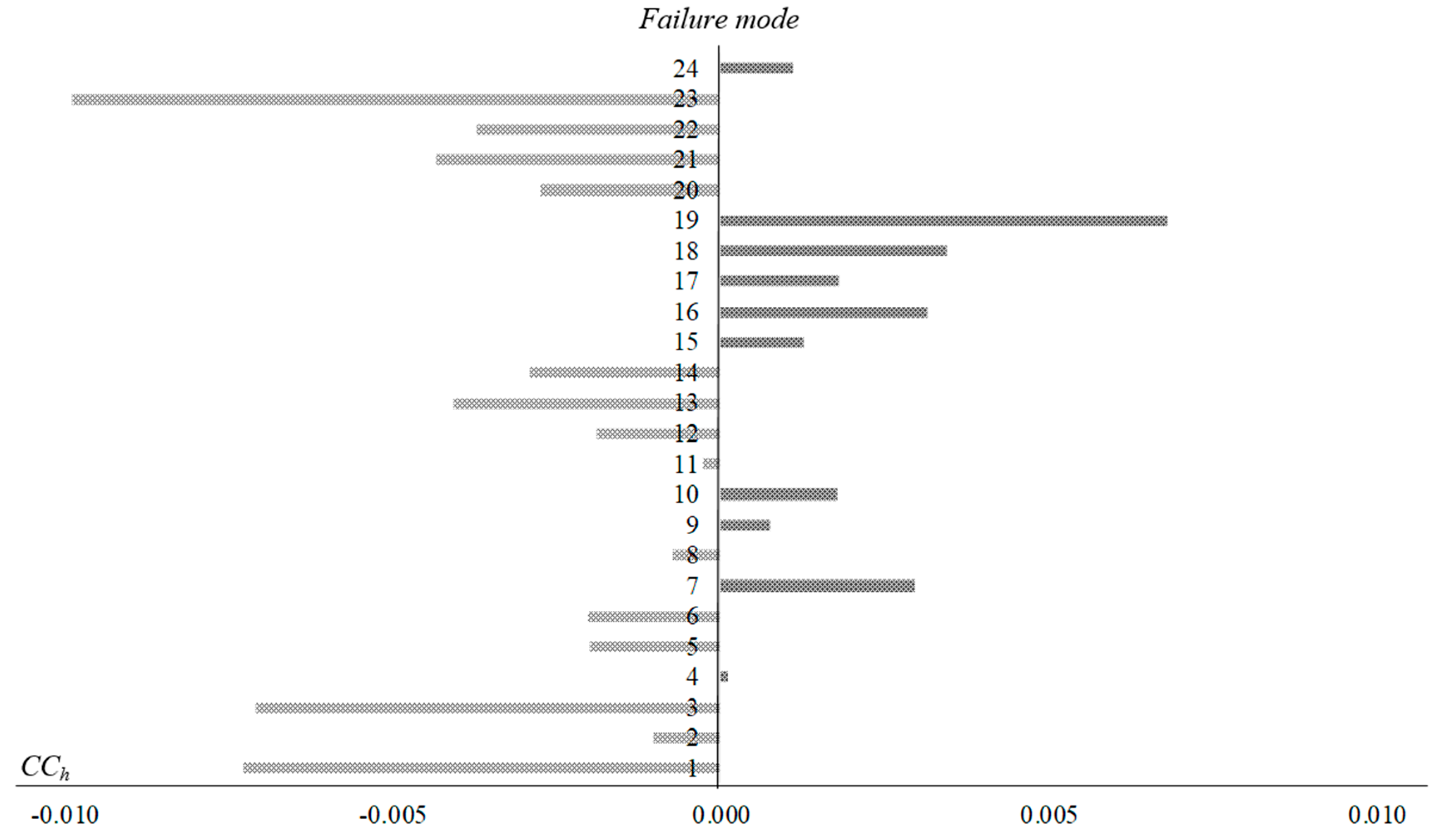
From the separation distances from FM₁₉ to PIS and NIS, it can be understood that this failure mode was the riskiest. Since FM₁₉ was closest to PIS (d₁₉^* = 0.527) in all failure modes and farthest from NIS (d₁₉⁻ = 0.385), it ranked first in the final result. Using the FMEA model developed, the company can quickly determine the improvement priorities of failure modes and develop corresponding risk management measures. Figure 1 shows the relative distances and positions of all failure modes; the bar graph indicates the approach coefficient of each failure mode, based on 0, and the failure mode developed toward the right indicates high risk. The study shows that all failure modes with CC_i > 0 should be prioritized because they were closer to the PIS.

There are many types of audio equipment, and the design structure and the way it is constructed are very complicated. The audio category of the V300 model is the most suitable for the public. It is necessary to conduct a careful failure assessment before the product goes on the market. As can be seen from the results of R-TOPSIS-AL, the key failure modes were classified as poor audio output quality, including quality abnormalities at high pitch (FM₁₉ and FM₁₈), vibrato problems (FM₁₆), and poor speaker impedance curves (FM₁₇). These problems are easily found when consumers use them, seriously affecting the enjoyment of hearing, thereby losing confidence in the brand. Eliminating these critical potential failure modes must rely on the engineer’s monitoring and control of the process. First of all, the treble voice coils, the sound films, and the terminals must be accurately positioned for installation. Additionally, the welding operators must have rigorous training to perform the job. At the time of detection, the treble must be tested with a 100% electroacoustic tester to test the treble frequency curve. In addition to the treble abnormality, the audio sound box assembly failure (FM₇) was also one of the key failure modes, and the poor internal resonance effect of the sound causes quality inconsistency.

To illustrate that the proposed model improved the traditional FMEA, the traditional FMEA method based on the RPN calculation was tested against the proposed model for comparison. Firstly, Model 1 involved a conventional FMEA model in which RPN values were obtained by multiplying S, O, and D, and the weights of the RPN elements were considered to be equal. Experts rated the different risk factors for all failure modes using an evaluation value from 1–10. The evaluation values of the 10 experts were integrated by arithmetic averaging. Model 2 involved a combination of the R-BWM and R-TOPSIS-AL methods.

Table 9. Failure mode rankings of the two FMEA models. R-BWM—rough best worst method.

Failure Mode	Conventional FMEA		Proposed Model R-BWM + R-TOPSIS-AL
FMh	RPN	Rank	CCh	Rank
FM1	36.504	17	−0.007	23
FM2	52.864	5	−0.001	13
FM3	28.704	19	−0.007	22
FM4	45.675	9	0.000	10
FM5	40.194	15	−0.002	15
FM6	49.140	7	−0.002	16
FM7	44.616	12	0.003	4
FM8	70.528	2	−0.001	12
FM9	47.850	8	0.001	9
FM10	58.240	4	0.002	6
FM11	43.750	13	0.000	11
FM12	63.504	3	−0.002	14
FM13	43.500	14	−0.004	20
FM14	45.500	10	−0.003	18
FM15	49.700	6	0.001	7
FM16	45.276	11	0.003	3
FM17	28.350	20	0.002	5
FM18	32.000	18	0.003	2
FM19	108.783	1	0.007	1
FM20	19.824	22	−0.003	17
FM21	20.736	21	−0.004	21
FM22	37.312	16	−0.004	19
FM23	7.896	24	−0.010	24
FM24	15.456	23	0.001	8
Correlation coefficient		0.3957		1

shows the results and rankings obtained using the two FMEA models. The traditional RPN range is from 1–1000, where a larger value indicates a greater risk of failure mode. The FM₁₉ had the highest RPN of 108.783. Obviously, the failure mode improvement priority ranking presented by the traditional FMEA method was significantly different from the proposed model. The Pearson correlation coefficient was used to calculate the correlation between the two groups, with a correlation of only about 40%.

BWM was widely used by researchers in recent years. Although the calculation of R-BWM needs to be solved by linear programming, the implementation process is intuitive and simple. According to the results of R-BWM, “severity” and “expected cost” were the key elements for evaluating the failure modes, which indicates that this study adding the expected cost to the evaluation factors of the FMEA was necessary. In general, it is impractical to put unlimited resources or most of the budget into risk prevention. If a company’s resource constraints in the real world are not considered, the analysis will be limited in practical applications. Also, any product should consider the reliability of the product from the R&D stage; otherwise, it will require additional maintenance costs and time during manufacturing and sales. The worst case is that consumers lose confidence in the brand. Previous studies proposed risk assessment methods such as fault tree analysis or hazard and operability studies; however, their processes of data survey and collection were time-consuming and cumbersome. The proposed model not only effectively integrates different expert opinions, but also greatly optimizes the calculation of traditional FMEA. The computational quality and time of R-TOPSIS-AL is not affected by the increase in criteria and alternatives.

Audio equipment directly affects people’s lives. The problem of audio output quality urgently needs to be improved. Engineers can consider using different construction methods or materials to eliminate these problems. The FMEA proposed in this study brings many benefits to the case company based on the hybrid MADM model, such as (i) improving product reliability and quality consistency, (ii) reducing R&D and manufacturing costs, significantly reducing time to market, (iii) improving customer satisfaction and lowering the cost of after-sales service, and (iv) documenting all FMEA data to continuously track and improve unresolved failure modes. Furthermore, the proposed FMEA can be extended to partners and suppliers of the case company, to further implement the total quality management on the supply chain. Although this study compensated for some of the limitations of the original FMEA method, there were still some limitations that should be addressed. The assessment of the failure modes is a qualitative investigation, and, in the future, more detection systems can be used to provide more timely measurement data to provide more information to assist the expert in judging the evaluation values of the failure modes. In addition, although the proposed model can help diagnose failures, troubleshooting still depends on trained professionals. At present, the interdependence between failure modes remains to be explored. In the future, decision-making trial and evaluation laboratory (DEMATEL) can be used to identify the dependence of failure modes, thus effectively eliminating the main causes of product failures.

References

- Chanamool, N.; Naenna, T. Fuzzy FMEA application to improve decision-making process in an emergency department. Appl. Soft Comput. 2016, 43, 441–453. [Google Scholar] [CrossRef]
- Kang, J.; Sun, L.; Sun, H.; Wu, C. Risk assessment of floating offshore wind turbine based on correlation-FMEA. Ocean Eng. 2017, 129, 382–388. [Google Scholar] [CrossRef]
- Lo, H.W.; Liou, J.J.; Huang, C.N.; Chuang, Y.C. A novel failure mode and effect analysis model for machine tool risk analysis. Reliab. Eng. Syst. Saf. 2019, 183, 173–183. [Google Scholar] [CrossRef]
- Ghoushchi, S.J.; Yousefi, S.; Khazaeili, M. An extended FMEA approach based on the Z-MOORA and fuzzy BWM for prioritization of failures. Appl. Soft Comput. 2019, 81, 105505. [Google Scholar] [CrossRef]
- Lo, H.W.; Liou, J.J. A novel multiple-criteria decision-making-based FMEA model for risk assessment. Appl. Soft Comput. 2018, 73, 684–696. [Google Scholar] [CrossRef]
- Chang, K.H. Generalized multi-attribute failure mode analysis. Neurocomputing 2016, 175, 90–100. [Google Scholar] [CrossRef]
- Mohsen, O.; Fereshteh, N. An extended VIKOR method based on entropy measure for the failure modes risk assessment—A case study of the geothermal power plant (GPP). Saf. Sci. 2017, 92, 160–172. [Google Scholar] [CrossRef]
- Liou, J.J. New concepts and trends of MCDM for tomorrow—In honor of Professor Gwo-Hshiung Tzeng on the occasion of his 70th birthday. Technol. Econ. Dev. Econ. 2013, 19, 367–375. [Google Scholar] [CrossRef]
- Rezaei, J. Best-worst multi-criteria decision-making method. Omega 2015, 53, 49–57. [Google Scholar] [CrossRef]
- Kuo, T. A modified TOPSIS with a different ranking index. Eur. J. Oper. Res. 2017, 260, 152–160. [Google Scholar] [CrossRef]
- Lo, H.W.; Liou, J.J.; Wang, H.S.; Tsai, Y.S. An integrated model for solving problems in green supplier selection and order allocation. J. Clean. Prod. 2018, 190, 339–352. [Google Scholar] [CrossRef]
- US Department of Defense Washington, D.C. Procedures for Performing a Failure Mode Effects and Criticality Analysis; US MIL-STD-1629A; Department of Defense: Washington, DC, USA, 1980.
- International Electrotechnical Commission, Geneva. Analysis Techniques for System Reliability—Procedures for Failure Mode and Effect Analysis, Geneva; IEC 60812; International Electrotechnical Commission: Geneva, Switzerland, 1985. [Google Scholar]
- Automotive industry action group (AIAG). Potential Failure Mode and Effect Analysis (FMEA) Reference Manual, FMEA Reference Manual, 4th ed.; Automotive Industry Action Group (AIAG): Southfield, MI, USA, 2008. [Google Scholar]
- Seyed-Hosseini, S.M.; Safaei, N.; Asgharpour, M.J. Reprioritization of failures in a system failure mode and effects analysis by decision making trial and evaluation laboratory technique. Reliab. Eng. Syst. Saf. 2006, 91, 872–881. [Google Scholar] [CrossRef]
- Shahin, A. Integration of FMEA and the Kano model: An exploratory examination. Int. J. Qual. Reliab. Manag. 2004, 21, 731–746. [Google Scholar] [CrossRef]
- Chemweno, P.; Pintelon, L.; Van Horenbeek, A.; Muchiri, P. Development of a risk assessment selection methodology for asset maintenance decision making: An analytic network process (ANP) approach. Int. J. Prod. Econ. 2015, 170, 663–676. [Google Scholar] [CrossRef]
- Zhao, H.; You, J.X.; Liu, H.C. Failure mode and effect analysis using MULTIMOORA method with continuous weighted entropy under interval-valued intuitionistic fuzzy environment. Soft Comput. 2017, 21, 5355–5367. [Google Scholar] [CrossRef]
- Safari, H.; Faraji, Z.; Majidian, S. Identifying and evaluating enterprise architecture risks using FMEA and fuzzy VIKOR. J. Intell. Manuf. 2016, 27, 475–486. [Google Scholar] [CrossRef]
- Wang, L.E.; Liu, H.C.; Quan, M.Y. Evaluating the risk of failure modes with a hybrid MCDM model under interval-valued intuitionistic fuzzy environments. Comput. Ind. Eng. 2016, 102, 175–185. [Google Scholar] [CrossRef]
- Ahn, J.; Noh, Y.; Park, S.H.; Choi, B.I.; Chang, D. Fuzzy-based failure mode and effect analysis (FMEA) of a hybrid molten carbonate fuel cell (MCFC) and gas turbine system for marine propulsion. J. Power Sources 2017, 364, 226–233. [Google Scholar] [CrossRef]
- Fattahi, R.; Khalilzadeh, M. Risk evaluation using a novel hybrid method based on FMEA, extended MULTIMOORA, and AHP methods under fuzzy environment. Saf. Sci. 2018, 102, 290–300. [Google Scholar] [CrossRef]
- Zhou, Q.; Thai, V.V. Fuzzy and grey theories in failure mode and effect analysis for tanker equipment failure prediction. Saf. Sci. 2016, 83, 74–79. [Google Scholar] [CrossRef]
- Pawlak, Z. Rough Sets: Theoretical Aspects of Reasoning about Data; Springer Science & Business Media: Berlin, Germany, 2012; Volume 9. [Google Scholar]
- Pamučar, D.; Gigović, L.; Bajić, Z.; Janošević, M. Location selection for wind farms using GIS multi-criteria hybrid model: An approach based on fuzzy and rough numbers. Sustainability 2017, 9, 1315. [Google Scholar] [CrossRef]
- Stević, Ž.; Pamučar, D.; Kazimieras Zavadskas, E.; Ćirović, G.; Prentkovskis, O. The selection of wagons for the internal transport of a logistics company: A novel approach based on rough BWM and rough SAW methods. Symmetry 2017, 9, 264. [Google Scholar] [CrossRef]
- Stević, Ž.; Pamučar, D.; Subotić, M.; Antuchevičiene, J.; Zavadskas, E. The location selection for roundabout construction using Rough BWM-Rough WASPAS approach based on a new Rough Hamy aggregator. Sustainability 2018, 10, 2817. [Google Scholar] [CrossRef]
- Stević, Ž.; Đalić, I.; Pamučar, D.; Nunić, Z.; Vesković, S.; Vasiljević, M.; Tanackov, I. A new hybrid model for quality assessment of scientific conferences based on Rough BWM and SERVQUAL. Scientometrics 2019, 119, 1–30. [Google Scholar] [CrossRef]
- Lo, H.W.; Liou, J.J.; Tzeng, G.H. Comments on “Sustainable recycling partner selection using fuzzy DEMATEL-AEW-FVIKOR: A case study in small-and-medium enterprises”. J. Clean. Prod. 2019, 228, 1011–1012. [Google Scholar] [CrossRef]
Figure 1.
Closeness coefficients of 24 failure modes.