Real-Time Optimization and Control of Nonlinear Processes Using Machine Learning

Abstract

Machine learning has attracted extensive interest in the process engineering field, due to the capability of modeling complex nonlinear process behavior. This work presents a method for combining neural network models with first-principles models in real-time optimization (RTO) and model predictive control (MPC) and demonstrates the application to two chemical process examples. First, the proposed methodology that integrates a neural network model and a first-principles model in the optimization problems of RTO and MPC is discussed. Then, two chemical process examples are presented. In the first example, a continuous stirred tank reactor (CSTR) with a reversible exothermic reaction is studied. A feed-forward neural network model is used to approximate the nonlinear reaction rate and is combined with a first-principles model in RTO and MPC. An RTO is designed to find the optimal reactor operating condition balancing energy cost and reactant conversion, and an MPC is designed to drive the process to the optimal operating condition. A variation in energy price is introduced to demonstrate that the developed RTO scheme is able to minimize operation cost and yields a closed-loop performance that is very close to the one attained by RTO/MPC using the first-principles model. In the second example, a distillation column is used to demonstrate an industrial application of the use of machine learning to model nonlinearities in RTO. A feed-forward neural network is first built to obtain the phase equilibrium properties and then combined with a first-principles model in RTO, which is designed to maximize the operation profit and calculate optimal set-points for the controllers. A variation in feed concentration is introduced to demonstrate that the developed RTO scheme can increase operation profit for all considered conditions.

1. Introduction

In the last few decades, chemical processes have been studied and represented with different models for real-time optimization (RTO) and model predictive control (MPC) in order to improve the process steady-state and dynamic performance. The available models range from linear to nonlinear and from first-principles models to neural network models, among others [1]. For many applications, first-principles models are the preferable choice, especially when applied with process systems methodologies [2]. However, first-principles models are difficult to maintain due to the variation of some parameters. Furthermore, it could be difficult or impractical to obtain first-principles models for large-scale applications [3]. As a well-tested alternative, machine learning method, especially neural network models are able to represent complicated nonlinear systems [4,5]. Neural networks fit the data in an input-output fashion using fully-connected layers within the hidden output layers [6]. However, due to their general structures, neural networks lack physical knowledge in their formulation. To alleviate the above problem, this work integrates neural network models with first-principles models. Specifically, first-principles models are used to represent the well-known part of the process and embedding physical knowledge in the formulation, while the complex nonlinear part of the process is represented with neural networks. This proposed hybrid formulation is then applied in the context of real-time optimization and model predictive control in two chemical processes.

The machine learning method has been part of process system engineering for at least 30 years in which the feed-forward neural network is the most classical structure found in the literature [7]. For instance, neural networks have been proposed as an alternative to first-principles models for the classical problems of process engineering [7], such as modeling, fault diagnosis, product design, state estimation, and process control. The neural network model has also gained much interest in the chemical engineering field, and more comprehensive reviews with detailed information on neural networks in chemical processes are available in [7,8]. For example, an artificial neural networks was applied to approximate pressure-volume-temperature data in refrigerant fluids [9]. Complex reaction kinetic data have been fitted using a large experimental dataset with neural networks to approximate the reaction rate and compared with standard kinetics methods, showing that neural networks can represent kinetic data at a faster pace [10]. Reliable predictions of the vapor-liquid equilibrium has been developed by means of neural networks in binary ethanol mixtures [11]. Studies on mass transfer have shown good agreements between neural network predictions and experimental data in the absorption performance of packed columns [12].

Since the applications with standard neural networks rely on fully-connected networks, the physical interpretation of the obtained model can be a difficult task. One solution is to integrate physical knowledge into the neural network model. For example, the work in [13] proposed a learning technique in which the neural network can be physically interpretable depending on the specifications. Similarly, the work in [14] designed a neural network with physical-based knowledge using hidden layers as intermediate outputs and prioritized the connection between inputs and hidden layers based on the effect of each input with the corresponding intermediate variables. Another method to add more physical knowledge into neural networks is to combine first-principles models with neural networks as hybrid modeling [15]. For instance, biochemical processes have been represented with mass balances for modeling the bioreactor system and with artificial neural networks for representing the cell population system [16]. Similarly, an experimental study for a bio-process showed the benefits of the hybrid approach in which the kinetic models of the reaction rates were identified with neural networks [17]. In crystallization, growth rate, nucleation kinetics, and agglomeration phenomena have been represented by neural networks, while mass, energy, and population balances have been used as a complement to the system’s behavior [18]. In industry, hybrid modeling using rigorous models and neural networks has also been tested in product development and process design [19]. However, most of the applications with hybrid modeling are limited to the open-loop case.

Real-time optimization (RTO) and model predictive control (MPC) are vital tools for chemical process performance in industry in which the process model plays a key role in their formulations [20,21]. RTO and MPC have been primarily implemented based on first-principles models, while the difference is that RTO is based on steady-steady models and MPC is based on dynamical models [20,21]. In both RTO and MPC, the performance depends highly on the accuracy of the process model. To obtain a more accurate model, machine learning methods have been employed within MPC [6] and within RTO [22], as well. In practice, it is common to use process measurements to construct neural network models for chemical processes. However, the obtained model from process operations may lack robustness and accuracy for parameter identification, as was shown in [23]. As a consequence, there has been significant effort to include hybrid models in process analysis, MPC, and process optimization [24,25,26,27,28,29,30] in order to reduce the dependency on data and infuse physical knowledge. At this stage, little attention has been paid to utilizing the full benefit of employing hybrid modeling in both the RTO and MPC layers.

Motivated by the above, this work demonstrates the implementation of a hybrid approach of combining a first-principles model and a neural network model in the RTO and MPC optimization problems. Specifically, the nonlinear part of the first-principles model is replaced by a neural network model to represent the complex, nonlinear term in a nonlinear process. We note that in our previous works, we developed recurrent neural network models from process data for use in MPC without using any information from a first-principles model or process structure in the recurrent neural network model formulation [4,5,31]. Furthermore, the previous works did not consider the use of neural network models to describe nonlinearities in the RTO layer and focused exclusively on model predictive control. In the present work, we use neural networks to describe nonlinearities arising in chemical processes and embed these neural network models in first-principles process models used in both RTO (nonlinear steady-state process model) and MPC (nonlinear dynamic process model), resulting in the use of hybrid model formulations in both layers. The rest of the paper is organized as follows: in Section 2, the proposed method that combines neural network with the first-principles model is discussed. In Section 3, a continuous stirred tank reactor (CSTR) example is utilized to illustrate the combination of neural network models and first-principles models in RTO and Lyapunov-based MPC, where the reaction rate equation is represented by a neural network model. In Section 4, an industrial distillation column is co-simulated in Aspen Plus Dynamics and MATLAB. A first-principles steady-state model of the distillation column is first developed, and a neural network model is constructed for phase equilibrium properties. The combined model is then used in RTO to investigate the performance of the proposed methodology.

2. Neural Network Model and Application

2.1. Neural Network Model

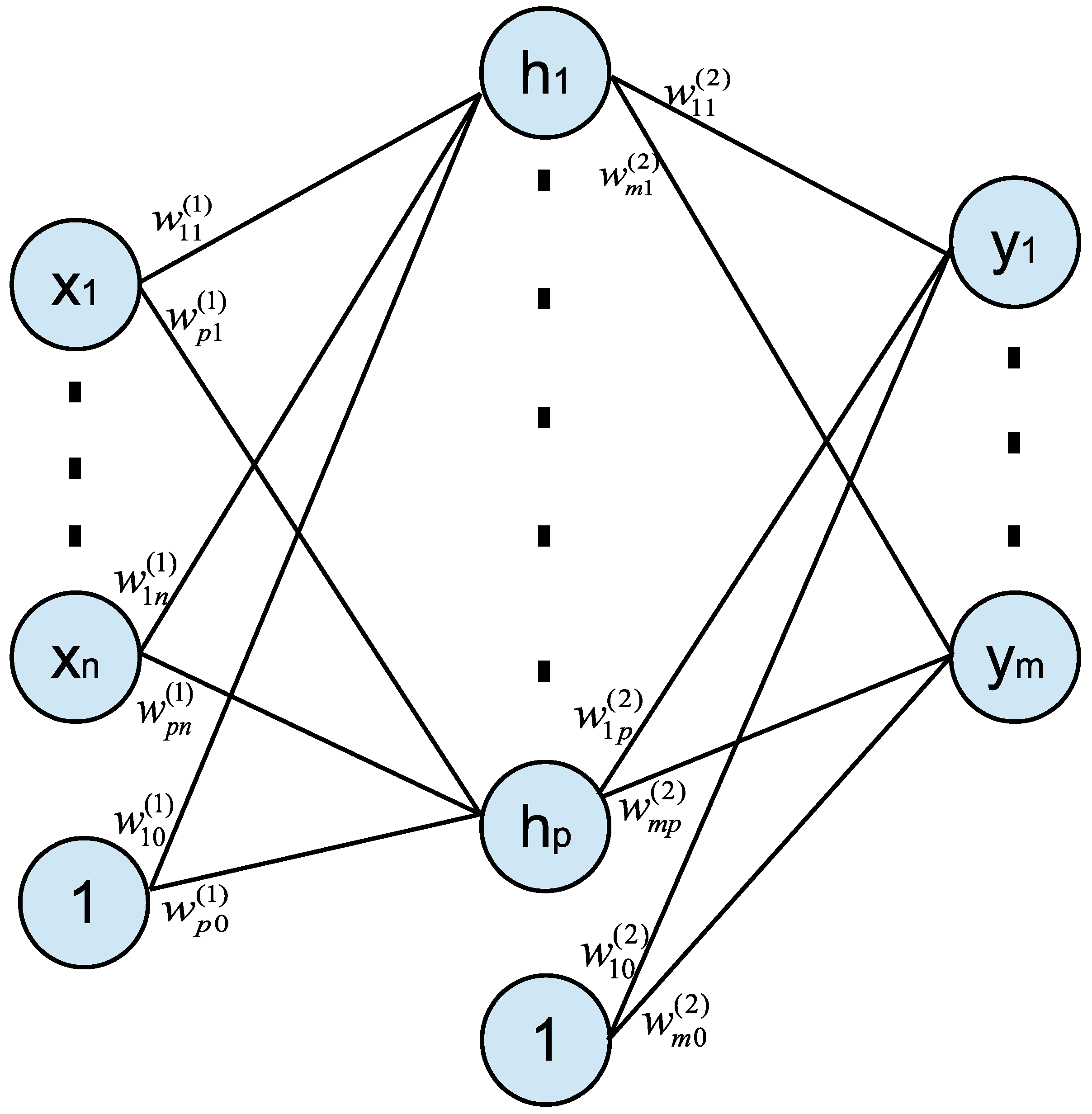
The neural network model is a nonlinear function $y=f_{NN}\left(x\right)$ with input vector $x=[x_1,x_2,\dots ,x_n]$ and output vector $y=[y_1,y_2,\dots ,y_m]$. Mathematically, a neural network function is defined as a series of functional transformations. The structure of a two-layer (one hidden-layer) feed-forward neural network is shown in Figure 1, where $h_1,h_2,\dots ,h_p$ are hidden neurons [32,33]. Specifically, the hidden neurons $h_j$ and the outputs $y_k$ are obtained by Equation (1):

$$\begin{array}{cc}\hfill h_j& ={\sigma }_1(\sum _{i=1}^n{w}_{ji}^{\left(1\right)}{x}_i+w_{j0}^{\left(1\right)}),j=1,2,\dots ,p\hfill \end{array}$$

(1a)

$$\begin{array}{cc}\hfill y_k& ={\sigma }_2(\sum _{i=1}^p{w}_{ki}^{\left(2\right)}{h}_i+w_{k0}^{\left(2\right)}),k=1,2,\dots ,m\hfill \end{array}$$

(1b)

where parameters $w_{ji}^{\left(1\right)}$ and $w_{ki}^{\left(2\right)}$ are weights in the first and the second layer and parameters $w_{j0}^{\left(1\right)}$ and $w_{k0}^{\left(2\right)}$ are biases. ${\sigma }_1$ and ${\sigma }_2$ are nonlinear element-wise transformations $\sigma :R^1\to R^1$, which are generally chosen to be sigmoid functions such as the logistic sigmoid $S\left(x\right)=1/(1+e^{-x})$ or hyperbolic tangent function $tanh\left(x\right)=2/(1+e^{-2x})-1$. Each hidden neuron $h_j$ is calculated by an activation function ${\sigma }_1$ with a linear combination of input variables $x_i$. Each output variable $y_k$ is also calculated by an activation function ${\sigma }_2$ with a linear combination of hidden neurons $h_i$. Since the neural network models in this work are developed to solve regression problems, no additional output unit activation functions are needed. All the neural network models in this work will follow the structure discussed in this section.

Given a set of input vectors $\left\{x^n\right\}$ together with a corresponding set of target output vectors $\left\{{\widehat{y}}^n\right\}$ as a training set of N data points, the neural network model is trained by minimizing the following sum-of-squares error function [33]:

$$E\left(w\right)=\frac{1}{2}\sum _{n=1}^N{\parallel y(x^n,w)-{\widehat{y}}^n\parallel }^2$$

(2)

The proper weight vectors w are obtained by minimizing the above cost function via the gradient descent optimization method:

$$w^{\tau +1}=w^{\tau }-\eta \nabla E\left(w^{\tau }\right)$$

(3)

where $\tau$ labels the iteration, $\eta >0$ is known as the learning rate, and $\nabla E\left(w^{\tau }\right)$ is the derivative of the cost function with respect to weight w. The weight vectors are optimized by moving through weight space in a succession of Equation (3) with some initial value $w\left(0\right)$. The gradient of an error function $\nabla E\left(w\right)$ is evaluated by back propagation method. Additionally, data are first normalized, and then, k-fold cross-validation is used to separate the dataset into the training and validation set in order to avoid model overfitting.

2.2. Application of Neural Network Models in RTO and MPC

In the chemical engineering field, model fitting is a popular technique in both academia and industry. In most applications, a certain model formulation needs to be assumed first, and then, the model is fitted with experiment data. However, a good approximation is not guaranteed since the assumed model formulation may be developed based on deficient assumptions and uncertain mechanism, which lead to an inaccurate model. Alternatively, neural network model can be employed to model complex, nonlinear systems since neural networks do not require any a priori knowledge about the process and are able to fit any nonlinearity with a sufficient number of layers and neurons according to the universal approximation theorem [34]. The obtained neural network model can be used together with existing first-principles models. Specifically, the combination of the neural network model and first-principles model can be used in optimization problems, such as real-time optimization (RTO) and model predictive control (MPC).

2.2.1. RTO with the Neural Network Model

Real-time optimization (RTO) maximizes the economic productivity of the process subject to operational constraints via the continuous re-evaluation and alteration of operating conditions of a process [35]. The economically-optimal plant operating conditions are determined by RTO and sent to the controllers to operate the process at the optimal set-points [36].

Since RTO is an optimization problem, an explicit steady-state model is required in order to obtain optimal steady-states. First-principles models are commonly used in RTO; however, first-principles models may not represent the real process well due to model mismatch, and thus lead to non-optimal steady-states or even infeasible steady-states. In these cases, the machine learning method becomes a good solution to improve model accuracy. Specifically, a neural network model can be used to replace the complicated nonlinear part of the steady-state model to increase the accuracy of the first-principles model.

In general, the RTO problem is formulated as the optimization problem of Equation (4), where $x\in R^n$ is the state and $\widehat{x}\in R^m$ is part of the state. $g\left(\widehat{x}\right)$ is a nonlinear function of $\widehat{x}$, which is a part of the steady-state model.

$$\begin{array}{cc}\hfill \underset{x}{min}& costfunction\left(x\right)\hfill \\ \hfill \mathrm{s}.\mathrm{t}.& F(x,g\left(\widehat{x}\right))=0\hfill \\ \hfill & otherconstraints\hfill \end{array}$$

(4)

Since it is difficult to obtain an accurate functional form of $g\left(\widehat{x}\right)$, a neural network $F_{NN}\left(\widehat{x}\right)$ is developed using simulation data to replace $g\left(\widehat{x}\right)$ in Equation (4). Therefore, the RTO based on the integration of first-principles model and neural network model is developed as follows:

$$\begin{array}{cc}\hfill \underset{x}{min}& costfunction\left(x\right)\hfill \\ \hfill \mathrm{s}.\mathrm{t}.& F(x,F_{NN}\left(\widehat{x}\right))=0\hfill \\ \hfill & otherconstraints\hfill \end{array}$$

(5)

2.2.2. MPC with Neural Network Models

Model predictive control (MPC) is an advanced control technique that uses a dynamic process model to predict future states over a finite-time horizon to calculate the optimal input trajectory. Since MPC is able to account for multi-variable interactions and process constraints, it has been widely used to control constrained multiple-input multiple-output nonlinear systems [37]. Since MPC is an optimization problem, an explicit dynamic model is required to predict future states and make optimal decisions. First-principles models can be developed and used as the prediction model in MPC; however, first-principles models suffer from model mismatch, which might lead to offsets and other issues. Therefore, machine learning methods can be used to reduce model mismatch by replacing the complicated nonlinear part of the dynamic model with a neural network model.

In general, MPC can be formulated as the optimization problem of Equation (6), where the notations follow those in Equation (4) and $\dot{x}=F(x,g\left(\widehat{x}\right))$ is the first-principles dynamic process model.

$$\begin{array}{cc}\hfill \underset{u}{min}& costfunction(x,u)\hfill \\ \hfill \mathrm{s}.\mathrm{t}.& \dot{x}=F(x,g\left(\widehat{x}\right),u)\hfill \\ \hfill & otherconstraints\hfill \end{array}$$

(6)

Similar to Equation (5), a neural network $F_{NN}\left(\widehat{x}\right)$ is developed using simulation data to replace $g\left(\widehat{x}\right)$ in Equation (6). As a result, the MPC based on the integration of the first-principles model and neural network model is developed as follows:

$$\begin{array}{cc}\hfill \underset{u}{min}& costfunction(x,u)\hfill \\ \hfill \mathrm{s}.\mathrm{t}.& \dot{x}=F(x,F_{NN}\left(\widehat{x}\right),u)\hfill \\ \hfill & otherconstraints\hfill \end{array}$$

(7)

Remark 1.

To derive stability properties for the closed-loop system under MPC, additional stabilizing constraints can be employed within the MPC of Equation (7) (e.g., terminal constraints [38] and Lyapunov-based constraints [39]). In this work, a Lyapunov-based MPC (LMPC) is developed to achieve closed-loop stability in the sense that the close-loop state is bounded in a stability region for all times and is ultimately driven to the origin. The discussion and the proof of closed-loop stability under LMPC using machine learning-based models can be found in [4,31].

Remark 2.

All the optimization problems of MPC and RTO in this manuscript are solved using IPOPT, which is an interior point optimizer for large-scale nonlinear programs. The IPOPT solver was run on the OPTI Toolbox in MATLAB. It is noted that the global optimum of the nonlinear optimization problem is not required in our case, since the control objective of MPC is to stabilize the system at its set-point, rather than to find the globally-optimal trajectory. The Lyapunov-based constraints can guarantee closed-loop stability in terms of convergence to the set-point for the nonlinear system provided that a feasible solution (could be a locally-optimal solution) to the LMPC optimization problem exists.

Remark 3.

In the manuscript, the MPC is implemented in a sample-and-hold fashion, under which the control action remains the same over one sampling period, i.e., $u\left(t\right)=u\left(x\left(t_k\right)\right)$, $\forall t\in [t_k,t_{k+1})$, where $t_{k+1}$ represents $t_k+\mathsf{\Delta }$ and Δ is the sampling period. Additionally, one possible way to solve the optimization problems of Equations (6) and (7) is to use continuous-time optimization schemes. This method has recently gained researchers attention and can be found in [40,41].

Remark 4.

In this work, the neural network is used to replace the nonlinear term in the first-principles model, for which it is generally difficult to obtain an accurate functional form from first-principles calculations. It should be noted that the neural network $F_{NN}\left(\widehat{x}\right)$ was developed as an input-output function to replace only a part (static nonlinearities) of the first-principles model, and thus does not replace the entire steady-state model or dynamic model.

3. Application to a Chemical Reactor Example

3.1. Process Description and Simulation

The first example considers a continuous stirred tank reactor (CSTR), where a reversible exothermic reaction $A\leftrightarrow B$ takes place [42,43]. After applying mass and energy balances, the following dynamic model is achieved to describe the process:

$$\begin{array}{cc}\hfill & {\displaystyle \frac{d{C}_A}{dt}}=\frac{1}{\tau }(C_{A_0}-C_A)-k_A{e}^{\frac{-E_A}{RT}}{C}_A+k_B{e}^{\frac{-E_B}{RT}}{C}_B\hfill \\ \hfill & {\displaystyle \frac{d{C}_B}{dt}}=-\frac{1}{\tau }{C}_B+k_A{e}^{\frac{-E_A}{RT}}{C}_A-k_B{e}^{\frac{-E_B}{RT}}{C}_B\hfill \\ \hfill & {\displaystyle \frac{dT}{dt}}=\frac{-\mathsf{\Delta }H}{\rho C_P}(k_A{e}^{\frac{-E_A}{RT}}{C}_A-k_B{e}^{\frac{-E_B}{RT}}{C}_B)+\frac{1}{\tau }(T_0-T)+\frac{Q}{\rho C_{P}V}\hfill \end{array}$$

(8)

In the model of Equation (8), $C_A$, $C_B$ are the concentrations of A and B in the reactor, and T is the temperature of the reactor. The feed temperature and concentration are denoted by $T_0$ and $C_{A_0}$, respectively. $k_A$ and $k_B$ are the pre-exponential factor for the forward reaction and reverse reaction, respectively. $E_A$ and $E_B$ are the activation energy for the forward reaction and reverse reaction, respectively. $\tau$ is the residence time in the reactor; $\mathsf{\Delta }H$ is the enthalpy of the reaction; and $C_P$ is the heat capacity of the mixture liquid. The CSTR is equipped with a jacket to provide heat to the reactor at rate Q. All process parameter values and steady-state values are listed in

Table 1. Parameter values and steady-state values for the continuous stirred tank reactor (CSTR) case study.

${\mathit{T}}_0=400$ K	$\mathit{\tau }=60$ s
$k_A=5000$ /s	$k_B={10}^6$ /s
$E_A=1\times {10}^4$ cal/mol	$E_B=1.5\times {10}^4$ cal/mol
$R=1.987$ cal/(mol K)	$\mathsf{\Delta }H=-5000$ cal/mol
$\rho =1$ kg/L	$C_P=1000$ cal/(kg K)
$C_{A_0}=1$ mol/L	$V=100$ L
$C_{A_s}=0.4977$ mol/L	$C_{B_s}=0.5023$ mol/L
$T_{A_s}=426.743$ K	$Q_s=\mathrm{40,386}$ cal/s

. Additionally, it is noted that the second equation of Equation (8) for $C_B$ is unnecessary if $C_{A_0}$ is fixed due to $C_B=C_{A_0}-C_A$. This does not hold when $C_{A_0}$ is varying, and thus, the full model is used in this work for generality.

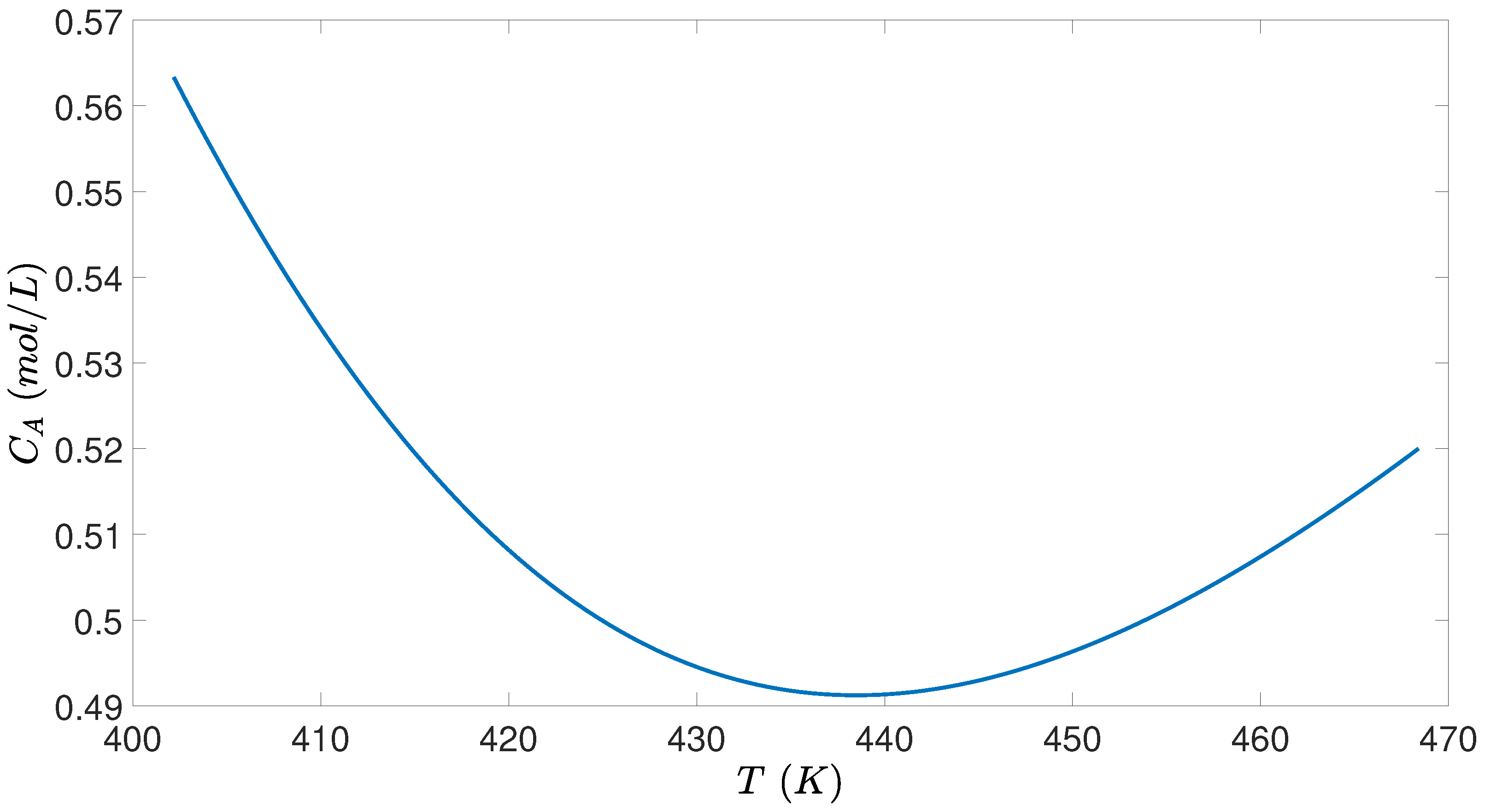
When the tank temperature T is too low, the reaction rate is maintained as slow such that the reactant A does not totally reacted during the residence time, and thus, the reactant conversion ($1-C_A/C_{A_0}$) is low. When the tank temperature T is too high, the reversible exothermic reaction equilibrium turns backwards so that the reactant conversion ($1-C_A/C_{A_0}$) also drops. As a result, there exists a best tank temperature to maximize the reactant conversion. Figure 2 shows the variation of the CSTR steady-state (i.e., concentration $C_A$ and temperature T) under varying heat input rate Q, where Q is not explicitly shown in Figure 2. Specifically, the minimum point of $C_A$ represents the steady-state of $C_A$ and T, under which the highest conversion rate (conversion rate = $1-C_A/C_{A_0}$) is achieved. Therefore, the CSTR process should be operated at this steady-state for economic optimality if no other cost is accounted for.

3.2. Neural Network Model

In the CSTR model of Equation (8), the reaction rate $r=k_A{e}^{\frac{-E_A}{RT}}{C}_A-k_B{e}^{\frac{-E_B}{RT}}{C}_B$ is a nonlinear function of $C_A$, $C_B$, and T. To obtain this reaction rate from experiment data, an assumption of the reaction rate mechanism and reaction rate function formulation is required. In practice, it could be challenging to obtain an accurate reaction rate expression using the above method if the reaction mechanism is unknown and the rate expression is very complicated.

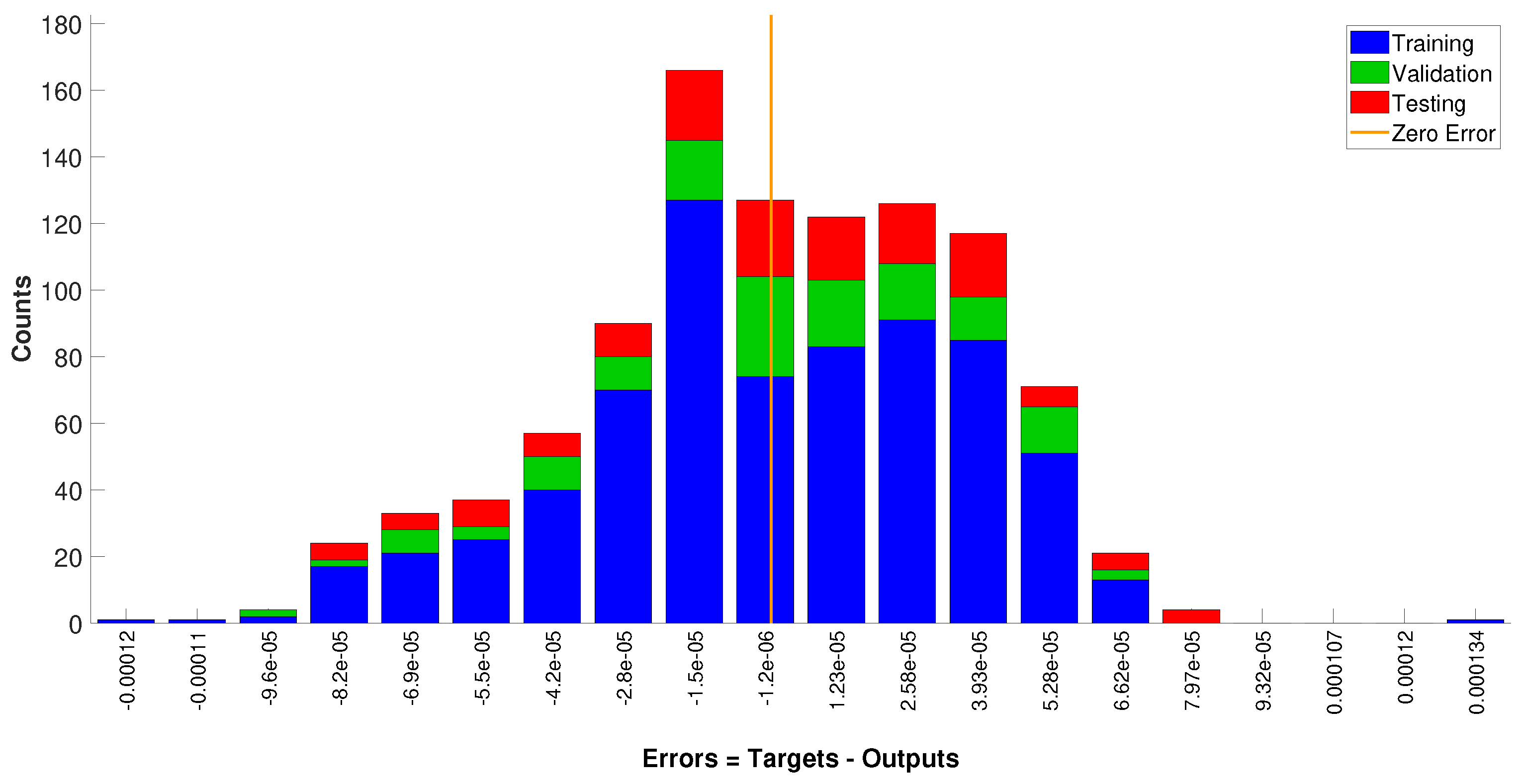
In this work, a neural network model is built to represent the reaction rate r as a function of $C_A$, $C_B$, and T (i.e., $r=F_{NN}(C_A,C_B,T)$), and then, the neural network model replaces the first-principles rate equation in the process model. Specifically, around eight million data were generated by the original reaction rate expression $r=k_A{e}^{\frac{-E_A}{RT}}{C}_A-k_B{e}^{\frac{-E_B}{RT}}{C}_B$ with different values of $C_A$, $C_B$, and T. The dataset was generated such that various reaction rates under different operating conditions (i.e., temperature, concentrations of A and B) were covered. The operating conditions were discretized equidistantly. Specifically, we tried the activation functions such as tanh, sigmoid, and ReLU for hidden layers and a linear unit and softmax function for the output layer. It is demonstrated that the choice of activation functions for the output layer significantly affected the performance of the neural network in a regression problem, while those for the hidden layers achieved similar results. $tanh\left(x\right)=2/(1+e^{-2x})-1$ was ultimately chosen as the activation function for the hidden layers, and a linear unit was used for the output layer since they achieved the best training performance with the mean squared error less than 10⁻⁷. Data were first normalized and then fed to the MATLAB Deep Learning toolbox to train the model. The neural network model had one hidden layer with 10 neurons. The parameters were trained using Levenberg–Marquardt optimization algorithm. In terms of the accuracy of the neural network model, the coefficient of determination $R^2$ was 1, and the error histogram of Figure 3 demonstrates that the neural network represented the reaction rate with a high accuracy, as can be seen from the error distribution (we note that error metrics used in classification problems like the confusion matrix, precision, recall, and f1-score were not applicable to the regression problems considered in this work). In the process model of Equation (8), the first-principles reaction rate term $k_A{e}^{\frac{-E_A}{RT}}{C}_A-k_B{e}^{\frac{-E_B}{RT}}{C}_B$ was replaced with the obtained neural network $F_{NN}(C_A,C_B,T)$. The integration of the first-principles model and the neural network model that was used in RTO and MPC will be discussed in the following sections.

Remark 5.

The activation function plays an important role in the neural network training process and may affect its prediction performance significantly. Specifically, in the CSTR example, since it is known that the reaction rate is generally in the form of exponential functions, we tried tanh and sigmoidactivation functions. It is demonstrated that both achieved the desired performance with mean squared error less than 10⁻⁷.

3.3. RTO and Controller Design

3.3.1. RTO Design

It is generally accepted that energy costs vary significantly compared to capital, labor, and other expenses in an actual plant. Therefore, in addition to productivity, it is important to account for energy cost in the real-time optimization of plant operation. Specifically, in this example, the heating cost was regarded as the entire energy cost since other energy costs may be lumped into the heating energy cost. The overall cost function is defined as follows:

$$totalcost=\frac{C_A}{C_{A_0}}+heatprice\times Q$$

(9)

Equation (9) attempts to find the balance between the reactant conversion and heat cost. A simple linear form was taken between Q and $C_A$ in this case study since it was sufficient to illustrate the relationship between energy cost and reactant conversion. The above total cost was optimized in real time to minimize the cost of the CSTR process, by solving the optimization problem of Equation (10).

$$\begin{array}{cc}\hfill \underset{C_A,C_B,T,Q}{min}& totalcost=\frac{C_A}{C_{A_0}}+heatprice\times Q\hfill \end{array}$$

(10a)

$$\begin{array}{cc}\hfill \mathrm{s}.\mathrm{t}.& 0=\frac{1}{\tau }(C_{A_0}-C_A)-F_{NN}(C_A,C_B,T)\hfill \end{array}$$

(10b)

$$\begin{array}{cc}\hfill & 0=-\frac{1}{\tau }{C}_B+F_{NN}(C_A,C_B,T)\hfill \end{array}$$

(10c)

$$\begin{array}{cc}\hfill & 0=\frac{-\mathsf{\Delta }H}{\rho C_P}{F}_{NN}(C_A,C_B,T)+\frac{1}{\tau }(T_0-T)+\frac{Q}{\rho C_{P}V}\hfill \end{array}$$

(10d)

$$\begin{array}{cc}\hfill & C_A\in [0,1]\hfill \end{array}$$

(10e)

$$\begin{array}{cc}\hfill & C_B\in [0,1]\hfill \end{array}$$

(10f)

$$\begin{array}{cc}\hfill & T\in [400,500]\hfill \end{array}$$

(10g)

$$\begin{array}{cc}\hfill & Q\in [0,{10}^5]\hfill \end{array}$$

(10h)

The constraints of Equation (10b), Equation (10c), and Equation (10d) are the steady-state models of the CSTR process, which set the time derivative of Equation (8) to zero and replace the reaction rate term by the neural network model built in Section 3.2. Since the feed concentration $C_{A_0}$ is 1 mol/L, $C_A$ and $C_B$ must be between 0 and 1 mol/L. The temperature constraint [400, 500] and energy constraint [0, 10⁵] are the desired operating conditions. At the initial steady-state, the heat price is 7 × 10⁻⁷, and the CSTR operates at T = 426.7 K, C_A = 0.4977 mol/L and Q = 40,386 cal/s. The performance is not compromised too much since C_A = 0.4977 mol/L is close to the optimum value C_A = 0.4912 mol/L, while the energy saving is considerable when Q = 40,386 cal/s is compared to the optimum value Q = 59,983 cal/s. In the presence of variation in process variables or heat price, RTO recalculates the optimal operating condition, given that the variation is measurable every RTO period. The RTO of Equation (10) is solved every RTO period, and then sends steady-state values to controllers as the optimal set-points for the next 1000 s. Since the CSTR process has a relatively fast dynamics, a small RTO period of 1000 s is chosen to illustrate the performance of RTO.

3.3.2. Controller Design

In order to drive the process to the optimal steady-state, a Lyapunov-based model predictive controller (LMPC) is developed in this section. The controlled variables are $C_A$, $C_B$, and T, and the manipulated variable is heat rate Q. The CSTR is initially operated at the steady-state $\left[C_{A_s}{C}_{B_s}{T}_s\right]$ = [0.4977 mol/L 0.5023 mol/L 426.743 K], with steady-state $Q_{j_s}=\mathrm{40,386}$ cal/s. At the beginning of each RTO period, a new set of steady-states are calculated, and then, the input and the states are represented in their deviation variable form as $u=Q-Q_s$ and $x^T=[C_A-C_{A_s}{C}_B-C_{B_s}T-T_s]$, such that the systems of Equation (8) together with $F_{NN}(C_A,C_B,T)$ can be written in the form of $\dot{x}=f\left(x\right)+g\left(x\right)u$. A Lyapunov function is designed using the standard quadratic form $V\left(x\right)=\mathrm{100,000}{x}_1^2+\mathrm{100,000}{x}_2^2+x_3^2$, and the parameters are chosen to ensure that all terms are of similar order of magnitude since temperature is varying in a much larger range compared to concentration. We characterize the stability region ${\mathsf{\Omega }}_{\rho }$ as a level set of Lyapunov function, i.e., ${\mathsf{\Omega }}_{\rho }=\left\{x\in R^3|V\left(x\right)\le \rho \right\}$. For the system of Equation (8), the stability region ${\mathsf{\Omega }}_{\rho }$ with $\rho =1000$ is found based on the above Lyapunov function V and the following controller $h\left(x\right)$ [44]:

$$h\left(x\right)=\left\{\begin{array}{ccc}-\frac{L_{f}V+\sqrt{L_f{V}^2+L_g{V}^4}}{{L_{g}V}^2}{L}_{g}V\hfill & if& L_{g}V\ne 0\hfill \\ 0\hfill & if& L_{g}V=0\hfill \end{array}\right.$$

(11)

where $L_{f}V\left(x\right)$ denotes the standard Lie derivative $L_{f}V\left(x\right):=\frac{\partial V\left(x\right)}{\partial x}f\left(x\right)$. The control objective is to stabilize $C_A$, $C_B$, and T in the reactor at its steady-state by manipulating the heat rate Q. A Lyapunov-based model predictive controller (LMPC) is designed to bring the process to the steady-state calculated by the RTO. Specifically, the LMPC is presented by the following optimization problem:

$$\begin{array}{cc}\hfill \underset{u\in S\left(\mathsf{\Delta }\right)}{min}& {\int }_{t_k}^{t_{k+N}}({∥\tilde{x}\left(\tau \right)∥}_{Q_c}^2+{∥u\left(\tau \right)∥}_{R_c}^2)d\tau \hfill \end{array}$$

(12a)

$$\begin{array}{cc}\hfill \mathrm{s}.\mathrm{t}.& \dot{\tilde{x}}\left(t\right)=f\left(\tilde{x}\left(t\right)\right)+g\left(\tilde{x}\left(t\right)\right)u\left(t\right)\hfill \end{array}$$

(12b)

$$\begin{array}{cc}\hfill & \tilde{x}\left(t_k\right)=x\left(t_k\right)\hfill \end{array}$$

(12c)

$$\begin{array}{cc}\hfill & u\left(t\right)\in U,\forall t\in [t_k,t_{k+N})\hfill \end{array}$$

(12d)

$$\begin{array}{cc}\hfill & \frac{\partial V\left(x\left(t_k\right)\right)}{\partial x}(f\left(x\left(t_k\right)\right)+g\left(x\left(t_k\right)\right)u\left(t_k\right))\le \frac{\partial V\left(x\left(t_k\right)\right)}{\partial x}(f\left(x\left(t_k\right)\right)+g\left(x\left(t_k\right)\right)h\left(x\left(t_k\right)\right))\hfill \end{array}$$

(12e)

where $\tilde{x}$ is the predicted state, N is the number of sampling periods within the prediction horizon, and $S\left(\mathsf{\Delta }\right)$ is the set of piece-wise constant functions with period $\mathsf{\Delta }$. The LMPC optimization problem calculates the optimal input trajectory over the entire prediction horizon $t\in [t_k,t_{k+N})$, but only applies the control action for the first sampling period, i.e., $u\left(t\right)=u\left(x\left(t_k\right)\right)$, $\forall t\in [t_k,t_{k+1})$. In the optimization problem of Equation (12), Equation (12a) is the objective function minimizing the time integral of ${∥\tilde{x}\left(\tau \right)∥}_{Q_c}^2+{∥u\left(\tau \right)∥}_{R_c}^2$ over the prediction horizon. Equation (12b) is the process model of Equation (8) in its deviation form and is used to predict the future states. A neural network $F_{NN}(x_1,x_2,x_3)$ is used to replace $k_A{e}^{\frac{-E_A}{RT}}{C}_A-k_B{e}^{\frac{-E_B}{RT}}{C}_B$ in Equation (8). Equation (12c) uses the state measurement $x\left(t_k\right)$ at $t=t_k$ as the initial condition $\tilde{x}\left(t_k\right)$ of the optimization problem. Equation (12d) defines the input constraints over the entire prediction horizon, where $U=[0-Q_s{10}^5-Q_s]$. The constraint of Equation (12e) is used to decrease $V\left(x\right)$ such that the state $x\left(t\right)$ is forced to move towards the origin. It guarantees that the origin of the closed-loop system is rendered asymptotically stable under LMPC for any initial conditions inside the stability region ${\mathsf{\Omega }}_{\rho }$. The detailed proof of closed-loop stability can be found in [39].

To simulate the dynamic model of Equation (8) numerically under the LMPC of Equation (12), we used the explicit Euler method with an integration time step of $h_c={10}^{-2}$ s. Additionally, the optimization problem of the LMPC of Equation (12) is solved using the solver IPOPT in the OPTI Toolbox in MATLAB with the following parameters: sampling period $\mathsf{\Delta }=5$ s; prediction horizon $N=10$. $Q_c=\left[100;010;005\times {10}^{-5}\right]$ and $R_c={10}^{-11}$ were chosen such that the magnitudes of the states and of the input in ${∥\tilde{x}\left(\tau \right)∥}_{Q_c}^2$ and ${∥u\left(\tau \right)∥}_{R_c}^2$ have the similar order.

3.4. Simulation Results

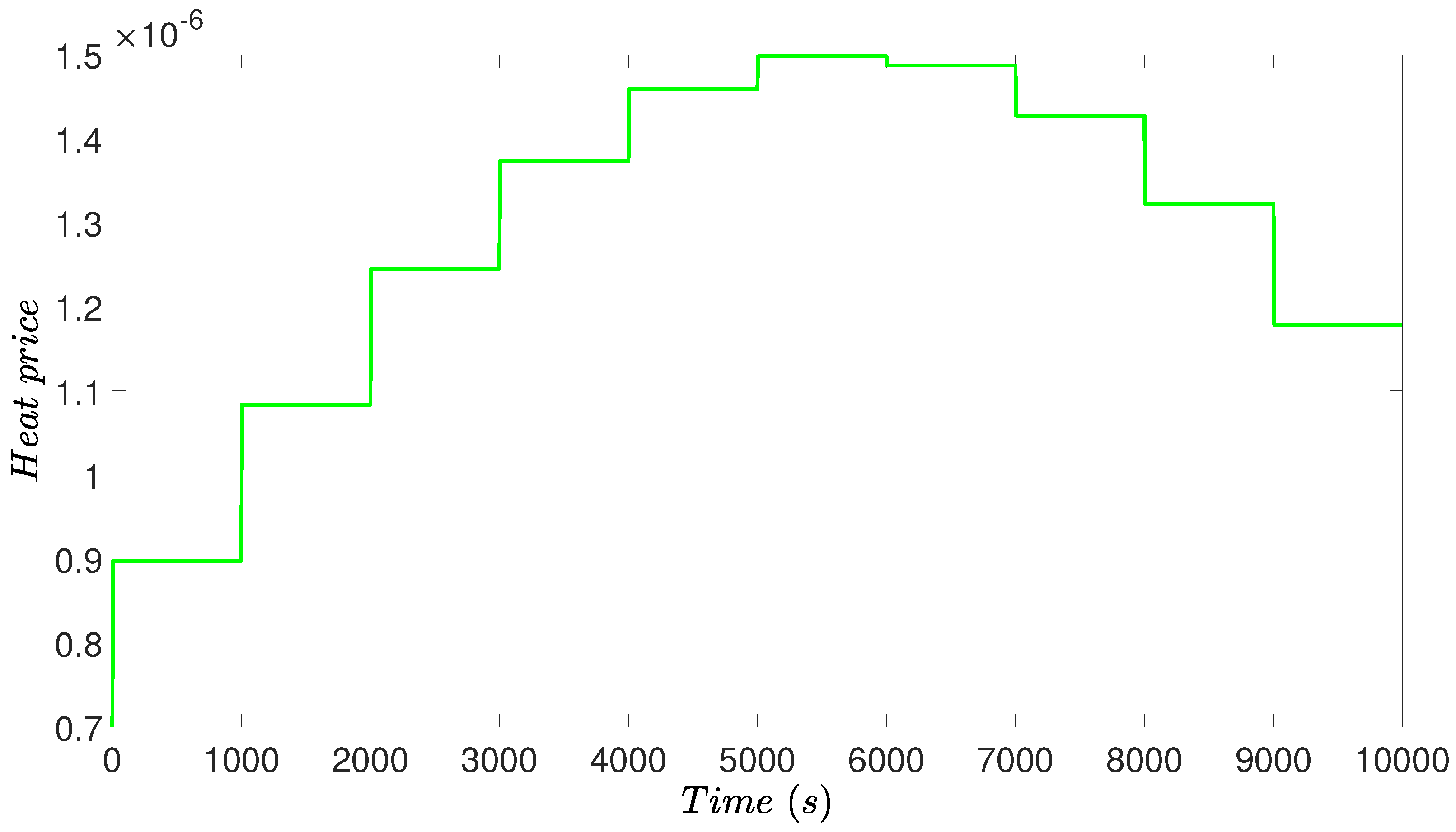
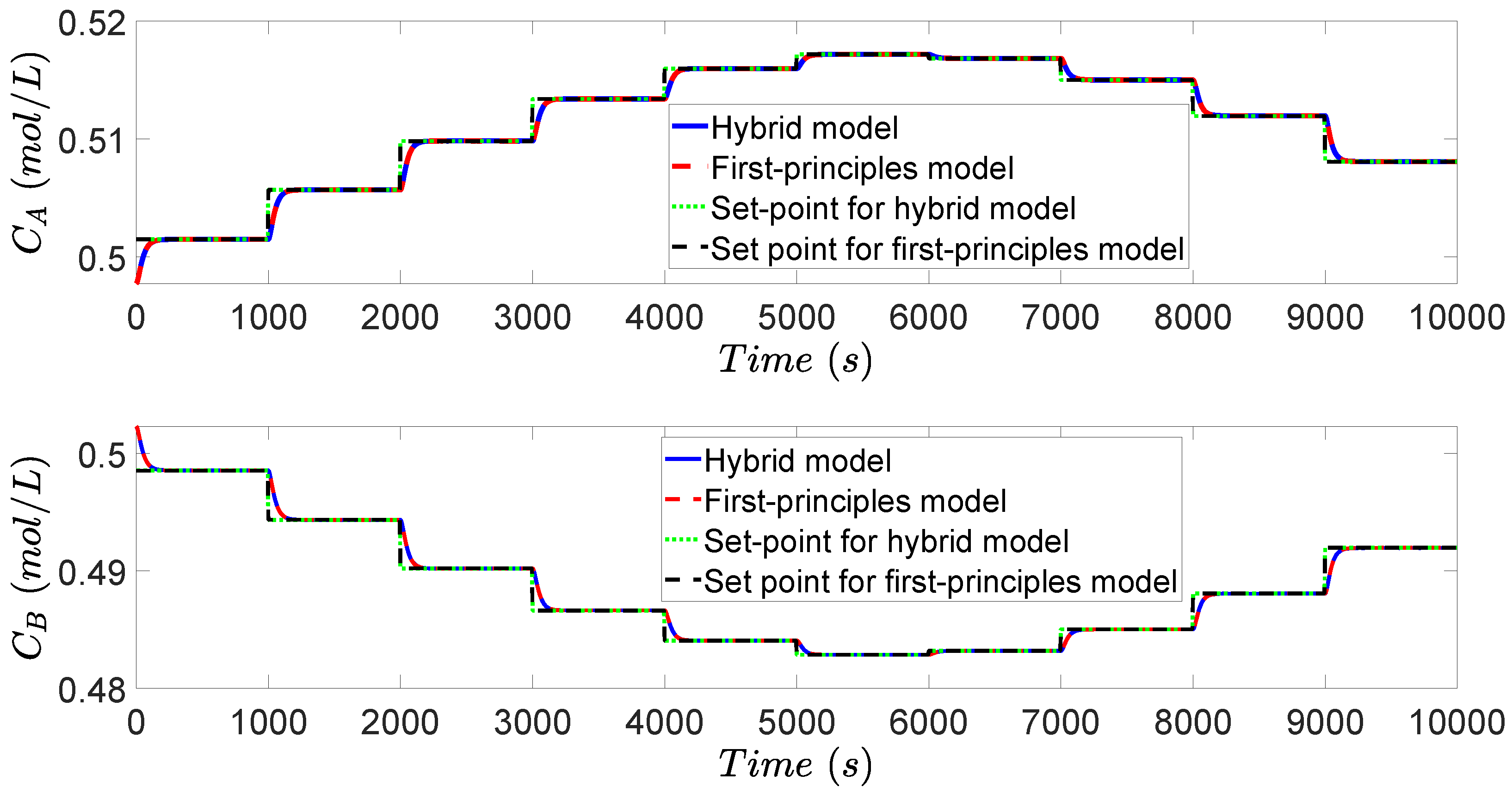
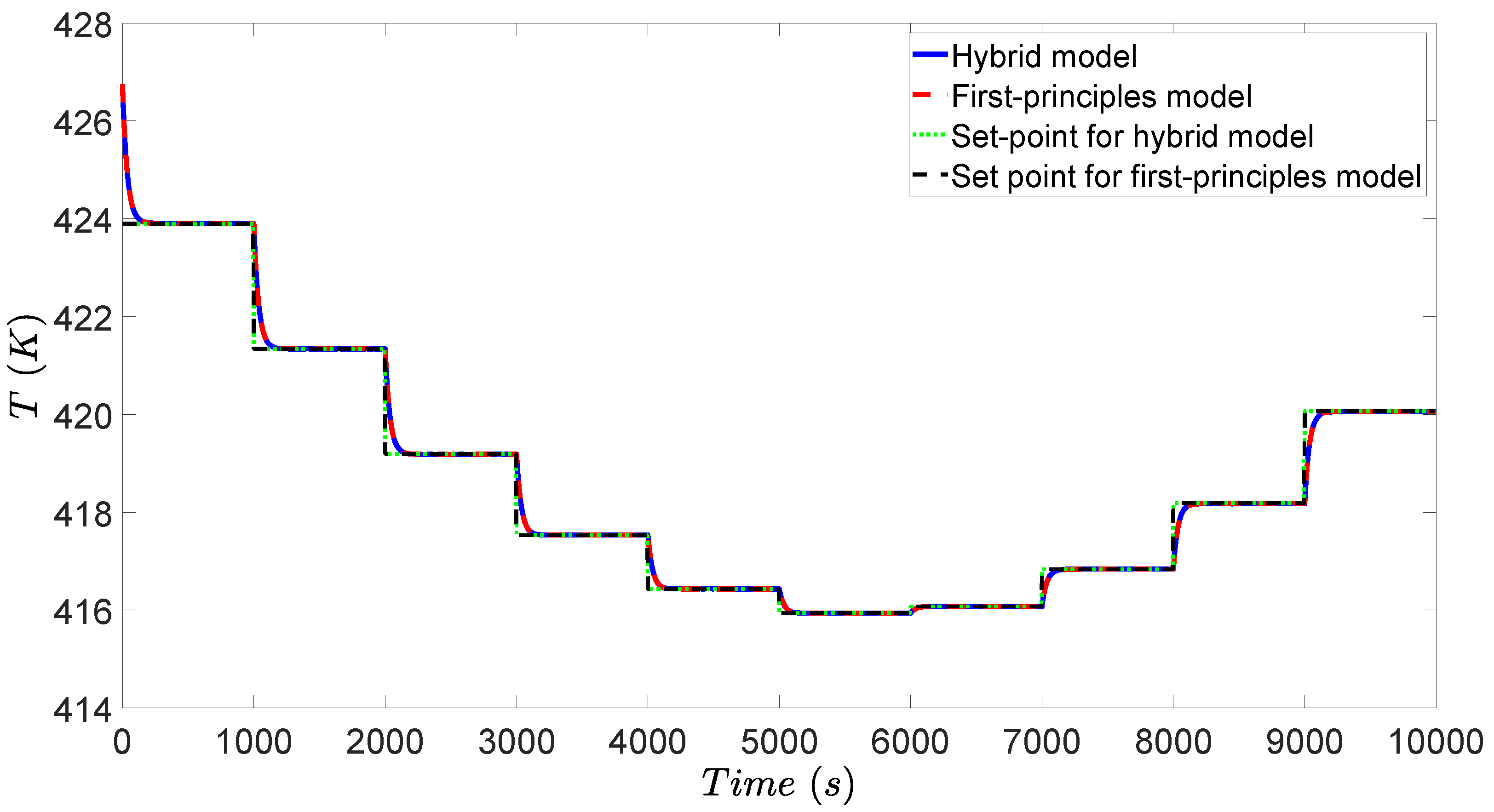
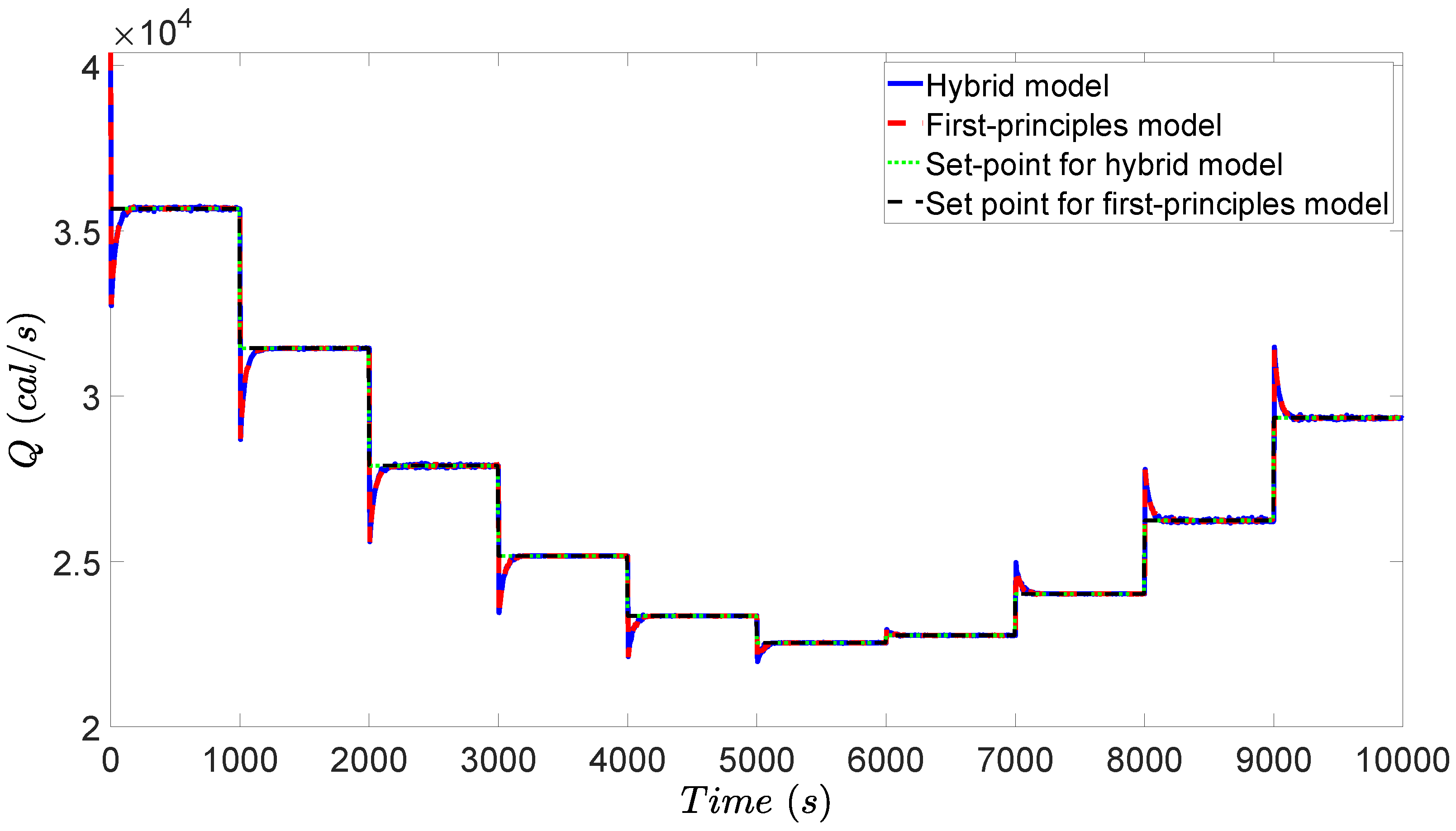
In the simulation, a variation of heat price is introduced to demonstrate the performance of the designed RTO and MPC. Since the heat price is changing as shown in Figure 4, the initial steady-state is no longer the optimal operating condition. The RTO of Equation (10) is solved at the beginning of each RTO period to achieve a set of improved set-points, which will be tracked by the MPC of Equation (12). With the updated set-points, the CSTR process keeps adjusting operating conditions accounting for varying heat price. After the controller receives the set-points, the MPC of Equation (12) calculates input u to bring x to the new set-point, and finally, both state x and input u are maintained at their new steady-states. The concentration profiles, temperature profile, and heat rate profile are shown in Figure 5, Figure 6 and Figure 7.

During the first half of the simulation, heat price rises up to a doubled value. Considering the increasing heat price, the operation tends to decrease the heat rate to reduce the energy cost, while compromising the reactant conversion. Therefore, the energy cost and reactant conversion will be balanced by RTO to reach a new optimum. As demonstrated in Figure 5, $C_A$ increases and $C_B$ decreases during the first half of simulation, which implies that less reactant A is converted to product B in the tank. The reactor temperature also drops as shown in Figure 6, which corresponds to the reducing heat rate as shown in Figure 7.

Total cost is calculated by Equation (9) using state measurements of $C_A$ and Q from the closed-loop simulation and is plotted in Figure 8. The total cost with fixed steady-state is also calculated and plotted for comparison. After the heat price starts to increase, both total costs inevitably increase. Since RTO keeps calculating better steady-states compared to the initial steady-state, the total cost under RTO increases less than the simulation without RTO. The total cost is integrated with time to demonstrate the difference in cost increment, using Equation (13).

$$costincrease={\int }_0^{t_{final}}\parallel totalcost-initialcost\parallel dt$$

(13)

where $initialcost=0.526$ and $t_{final}=$ 10,000 s. The ratio of cost increment between simulations with RTO and without RTO is $195:241$. Although the operating cost increases because of rising heat price, RTO reduces the cost increment by approximately a factor of 1/5, when compared to the fixed operating condition without RTO.

The combination of neural network models and first-principles models works well in both RTO and MPC. Additionally, it is shown in Figure 5, Figure 6 and Figure 7 that the RTO with the combined first-principles/neural-network model calculates the same steady-state when compared to the RTO with a pure first-principles model. Moreover, the MPC also drives all the states to the set-points without offset when the MPC uses the combination of a neural network model with a first-principles model. In this case study, the neural network model is accurate such that the combination of neural network and first-principles model attains almost the same closed-loop result as the pure first-principles model (curves overlap when plotted in the same figure as is done in Figure 5, Figure 6 and Figure 7, where the blue curve denotes the solution under MPC with the combined first-principles/neural network model, the red curve denotes the solution under MPC with the first-principles model, the green curve denotes the set-points calculated by RTO with the hybrid model, and the black curve denotes the set-points calculated by RTO with the first-principles model). Additionally, we calculated the accumulated relative error (i.e., $E=\frac{{\int }_{t=0}^{t=\mathrm{10,000}s}|T_f-T_h|dt}{{\int }_{t=0}^{t=\mathrm{10,000}s}{T}_{f}dt}$) between the temperature curves (Figure 6) under the first-principles model (i.e., $T_f$) and under the hybrid model (i.e., $T_h$) over the entire operating period from $t=0$ to $t=\mathrm{10,000}$ s. It was obtained that $E=4.98\times {10}^{-6}$, which is sufficiently small. This implies that the neural network successfully approximated the nonlinear term of reaction rate. In practice, neural network could be more effective when the reaction rate is very complicated and depends on more variables and the reaction mechanism is unknown.

4. Application to a Distillation Column

4.1. Process Description, Simulation, and Model

4.1.1. Process Description

A simple binary separation of propane from isobutane in a distillation column was used for the second case study [45]. Aspen Plus (Aspen Technology, Inc., Bedford, MA, USA) and Aspen Plus Dynamics V10.0 were utilized to perform high-fidelity dynamic simulation for the distillation column. Specifically, Aspen Plus uses the mass and energy balances to calculate the steady-state of the process based on a process flowsheet design and carefully-chosen thermodynamic models. After the steady-state model is solved in Aspen Plus, it can be exported to a dynamic model in Aspen Plus Dynamics, which runs dynamic simulations based on the obtained steady-state models and detailed process parameters [46,47].

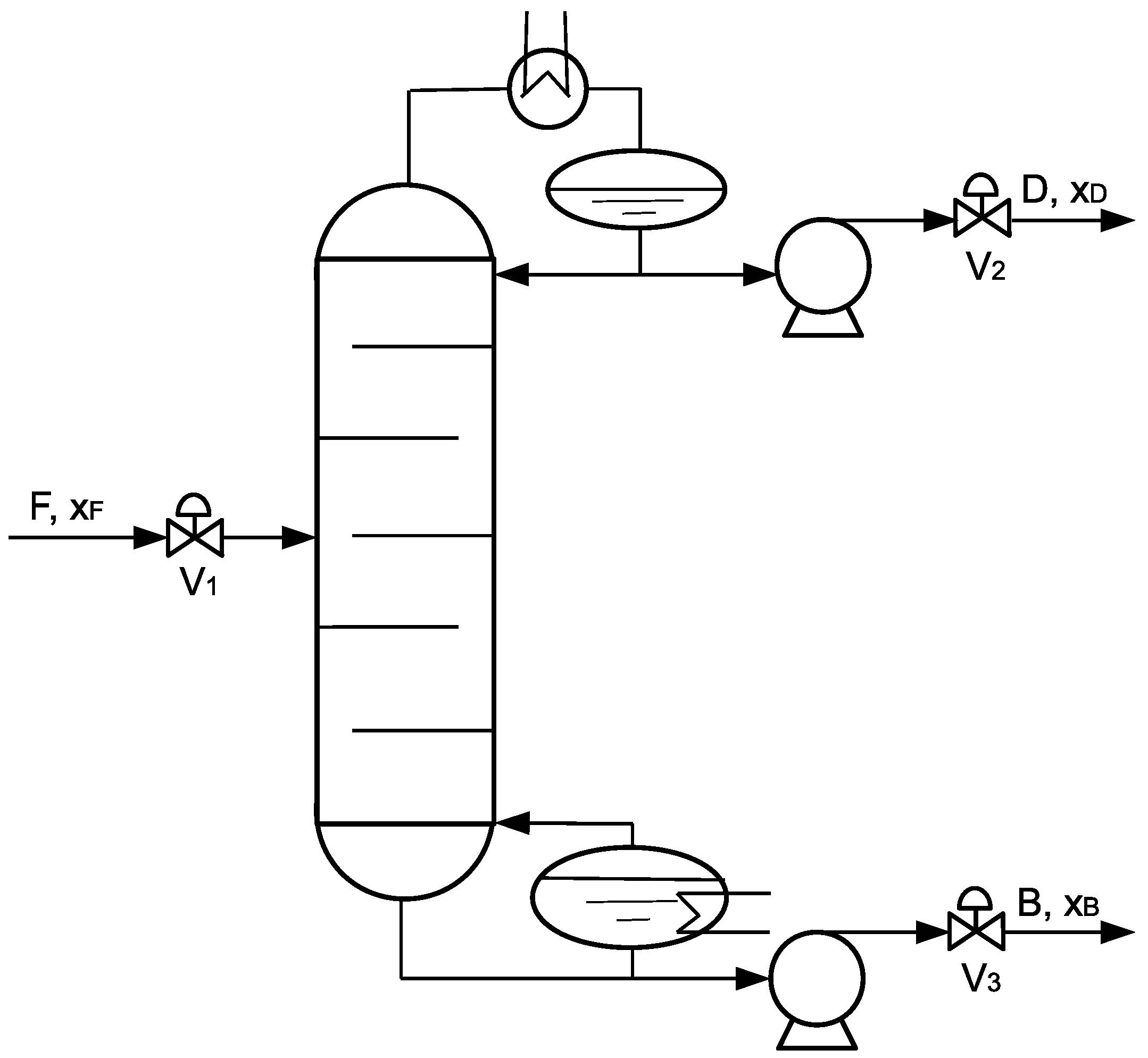
A schematic of the distillation process is shown in Figure 9. The feed to the separation process was at 20 atm, 322 K and 1 kmol/s, with a propane mole fraction of 0.4 and an isobutane mole fraction of 0.6. After a valve controlling the feed flow rate, the feed enters the distillation column at Tray 14. The feed tray is carefully chosen to achieve the best separation performance and minimum energy cost, as discussed in [45]. The column has 30 trays with a tray spacing of 0.61 m, and the diameter of the tray is 3.85 m and 4.89 m for the rectifying section and stripping section, respectively. At the initial steady-state, the distillate product has a propane mole fraction 0.98 and a flow rate 0.39 kmol, while the bottom product has a propane mole fraction 0.019 and a flow rate 0.61 kmol. The reflux ratio is 3.33, together with condenser heat duty −2.17 × 10⁷ W and reboiler heat duty 2.61 × 10⁷ W. The pressure at the top and bottom is 16.8 atm and 17 atm. Both the top and bottom products are followed by a pump and a control valve. All the parameters are summarized in

Table 2. Parameter values and steady-state values for the distillation column case study.

F = 1 kmol	${\mathit{x}}_{\mathit{F}}$ = 0.4
$T_F=322$ K	$P_F=20$ atm
q = 1.24	$N_F$ = 14
$N_T$ = 30	$Diamete{r}_{reboiler}=5.08$ m
$Lengt{h}_{reboiler}=10.16$ m	$Diamete{r}_{refluxdrum}=4.08$ m
$Lengt{h}_{refluxdrum}=8.16$ m
steady-state condition:	R = 3.33
$x_B=0.019$	$x_D=0.98$
$P_{bottom}=17$ atm	$P_{top}=16.8$ atm
B = 0.61 kmol/L	D = 0.39 kmol/L
$Q_{top}=-2.17\times {10}^7$ W	$Q_{bottom}=2.61\times {10}^7$ W

.

In our simulation, the involved components of propane and isobutane were carefully chosen, and the CHAO-SEA model was selected for the thermodynamic property calculation. The steady-state model was first built in Aspen Plus using the detailed information as discussed above and the parameters in Table 2. Then, the achieved steady-state simulation was exported to the dynamic model as a pressure-driven model, based on additional parameters such as reboiler size and drum size. After checking the open-loop response of the dynamic model, controllers will be designed in Section 4.3.2.

4.1.2. Process Model

In order to calculate the steady-state of the distillation process, an analytic steady-state model is developed in this section. Since the Aspen model cannot be used in the optimization problem explicitly, this analytic steady-state model will be used in the RTO.

The analytic steady-state model consists of five variables, which are the reflux ratio R, the distillate mole flow rate D, the bottom mole flow rate B, the distillate mole fraction $x_D$, and the bottom mole fraction $x_B$. For clarification, x is denoted as the mole fraction for the light component propane. Other parameters include feed conditions: feed molar flow rate F, feed mole fraction $x_F$, feed heat condition q; column parameters: total number of trays $N_T$, feed tray $N_F$; component property: relative volatility $\alpha$. Three equations were developed for the steady-state model.

The first equation $F_1(D,B)=0$ is the overall molar balance between feed and products, as shown in Equation (14).

$$F=D+B$$

(14)

The second equation $F_2(D,B,x_D,x_B)=0$ is the overall component balance of light component propane, as shown in Equation (15):

$$F{x}_F=D{x}_D+B{x}_B$$

(15)

The third equation applies the binary McCabe–Thiele method. The constant molar overflow assumptions of the McCabe–Thiele method were held in this case study: the liquid and vapor flow rates were constant in a given section of the column. Equilibrium was also assumed to be reached on each tray. The top tray was defined as the first tray. To apply the McCabe–Thiele method, the rectifying operating line (ROL), stripping operating line (SOL), and phase equilibrium were developed as follows:

Rectifying operating line (ROL):

$$y_{n+1}=\frac{R}{R+1}{x}_n+\frac{x_D}{R+1}$$

(16)

Stripping operating line (SOL):

$$y_{n+1}=\frac{RD+qF}{(R+1)D-(1-q)F}{x}_n+\frac{F-D}{(R+1)-(1-q)F}{x}_B$$

(17)

Phase equilibrium:

$$x_n=\frac{y_n}{\alpha -(\alpha -1)y_n}$$

(18)

where $\alpha =\frac{y_{C3}/x_{C3}}{y_{C4}/x_{C4}}=1.79$ is the approximate relative volatility between propane and isobutane at a pressure 16.9 atm, which is the mean of the top and bottom pressure.

The third equation $F_3(R,D,x_D,x_B)=0$ is expressed in Equation (19) below:

$$\begin{array}{cc}\hfill y_1& =x_D\hfill \end{array}$$

(19a)

$$\begin{array}{cc}\hfill x_n& =\frac{y_n}{\alpha -(\alpha -1)y_n}n=1,2\dots N_T\hfill \end{array}$$

(19b)

$$\begin{array}{cc}\hfill y_{n+1}& =\frac{R}{R+1}{x}_n+\frac{x_D}{R+1}n=1,2\dots N_F-1\hfill \end{array}$$

(19c)

$$\begin{array}{cc}\hfill y_{n+1}& =\frac{RD+qF}{(R+1)D-(1-q)F}{x}_n+\frac{F-D}{(R+1)-(1-q)F}{x}_{B}n=N_F,N_F+1\dots N_T-1\hfill \end{array}$$

(19d)

$$\begin{array}{cc}\hfill x_{N_T}& =x_B\hfill \end{array}$$

(19e)

The third equation $F_3(R,D,x_D,x_B)=0$ ties the distillate mole fraction $x_D$ to the bottom mole fraction $x_B$ by calculating both liquid and vapor mole fractions through all trays from top to bottom. Equation (19a) defines the vapor mole fraction $y_1$ on the first tray as the distillate mole fraction $x_D$. Then, the liquid mole fraction $x_1$ on the first tray can be calculated by the phase equilibrium of Equation (19b). Subsequently, the vapor mole fraction $y_2$ on the second tray is calculated by the ROL of Equation (19c). The calculation is repeated until $x_{14}$ and $y_{14}$ are obtained. Then, $y_{15}$ is calculated by the SOL of Equation (19d), instead of ROL. Then, $x_{15}$ can be calculated again by the phase equilibrium of Equation (19b). The above calculations are repeated until $x_{30}$ and $y_{30}$ are obtained, and $x_{30}=x_B$ since the liquid on the last tray is the bottom product. In this way, all the variables (i.e., R, D, $x_D$, $x_B$) have values that satisfy $F_3(R,D,x_D,x_B)=0$.

There are five variables R, D, B, $x_D$, $x_B$ and three equations $F_1$, $F_2$, $F_3$, which implies that there are two degrees of freedom. In order to determine the whole process operating condition, two more states need to be fixed, potentially by RTO. It is necessary to point out that the concentrations $x_i$ and $y_i$ on each tray can be calculated by Equation (19) if all five variables R, D, B, $x_D$, $x_B$ are determined. Additionally, if the equilibrium temperature-component curve $T=f_e\left(x\right)$ (bubble point curve) or $T=f_e\left(y\right)$ (dew point curve) are provided, then the temperature on each tray $T_i$ can also be calculated by simply using $T_i=f_e\left(x_i\right)$ or $T_i=f_e\left(y_i\right)$.

4.2. Neural Network Model

Phase equilibrium properties are usually nonlinear, and the first-principles models are often found to be inaccurate and demand modifications. In the above steady-state model, the phase equilibrium $x_n=\frac{y_n}{\alpha -(\alpha -1)y_n}$ of Equation (19b) assumes that relative volatility $\alpha$ is constant; however, the relative volatility $\alpha$ does not hold constant with varying concentration and pressure. Therefore, a more accurate model for phase equilibrium $x\sim y$ can improve the model performance. Similarly, dew point curve $T\sim y$ can be built from first-principles formulation upon Raoult’s Law and the Antoine equation. However, the Antoine equation is an empirical equation, and it is hard to relate saturated pressure with temperature accurately, especially for a mixture. As a result, the machine learning method can be used to achieve a better model to represent the phase equilibrium properties.

In this case study, a neural network $(x,T)=F_{NN}\left(y\right)$ was built, with one input (vapor phase mole fraction y) and two outputs (equilibrium temperature T and liquid phase mole fraction x). One thousand five hundred data of T, x, and y were generated by the Aspen property library and were then normalized and fed into the MATLAB Deep Learning toolbox. $tanh\left(x\right)=2/(1+e^{-2x})-1$ was chosen as the activation function. The neural network model had one hidden layer with five neurons. The parameters were trained according to Levenberg–Marquardt optimization, and the mean squared error for the test dataset was around 10⁻⁷. It is demonstrated in Figure 10 that the neural network model fits the data from the Aspen property library very well, where the blue solid curve is the neural network model prediction and the red curve denotes the Aspen model. Additionally, we calculated the accumulated relative error (i.e., $E=\frac{{\int }_{y=0}^{y=1}|T_f-T_h|dy}{{\int }_{y=0}^{y=1}{T}_{f}dy}$) between the temperature curves (Figure 10) under the Aspen model (i.e., $T_f$) and under the neural network model (i.e., $T_h$) and $E=2.32\times {10}^{-6}$; the result was similar for the liquid mole fraction curves. This sufficiently small error implies that the neural network model successfully approximated the nonlinear behavior of the thermodynamic properties. Additionally, the coefficient of determination $R^2$ was 1, and the error histogram of Figure 11 demonstrated that the neural network model represented the thermodynamic properties with great accuracy.

After training the neural network model, the first-principles phase equilibrium expression $x_n=\frac{y_n}{\alpha -(\alpha -1)y_n}$ in Equation (19b) is replaced by the neural network phase equilibrium expression $x_n=F_{NN,1}\left(y_n\right)$, and then, the integrated model of first-principles model and neural network model is used in RTO as discussed in the following sections. In addition, the second output of the neural network model $T_n=F_{NN,2}\left(y_n\right)$ can be combined together with Equation (19) to calculate the temperature on each tray, which will be used later to calculate the set-points for the controllers.

4.3. RTO and Controller Design

4.3.1. RTO Design

Since the process has two degrees of freedom, the operating condition has not been determined. An RTO was designed for the distillation process to obtain the optimal operating condition. Since RTO needs an objective function, a profit was developed to represent the operation profit. According to the products, feed, and energy price in [45], the profit is defined by Equation (20).

$$\begin{array}{cc}\hfill Profit& =pric{e}_{top}D+pric{e}_{bottom}B-pric{e}_{feed}F-pric{e}_{energy}Q\hfill \\ \hfill & =pric{e}_{top}D+pric{e}_{bottom}B-pric{e}_{feed}F-pric{e}_{energy}\left(L(R+1)F\right)\hfill \\ \hfill & =Profit(R,D,B,x_D,x_B)\hfill \end{array}$$

(20)

The profit equals the profit of product subtracting the cost of feed and energy. The profit that will be used in RTO is represented as a function of R, D, B, $x_D$,$x_B$. As a result, heat duty Q of both the condenser and reboiler is approximated by $Q=L(R+1)F$, where $L=1.29\times {10}^7$ J/kmol is the molar latent heat of the mixture. Moreover, mass-based prices are changed to mole-based prices because all flow rates are mole-based. The price of the top distillate rises linearly as the mole fraction $x_D$ increases in order to demonstrate that the higher purity product has a higher price.

$$\begin{array}{cc}\hfill pric{e}_{top}& =(0.528+(x_D-0.97)) \$/\mathrm{kg}\times 44.1 \mathrm{kg}/\mathrm{kmol}=23.29+44.1(x_D-0.97) \$/\mathrm{kmol}\hfill \\ \hfill pric{e}_{bottom}& =0.264 \$/\mathrm{kg}\times 58.1 \mathrm{kg}/\mathrm{kmol}=15.34 \$/\mathrm{kmol}\hfill \\ \hfill pric{e}_{feed}& =0.264 \$/\mathrm{kg}\times 52.5 \mathrm{kg}/\mathrm{kmol}=13.86 \$/\mathrm{kmol}\hfill \\ \hfill pric{e}_{energy}& =6.11\times {10}^{-8} \$/\mathrm{J}\hfill \end{array}$$

(21)

To maximize the operation profit, the RTO problem is formulated as Equation (22).

$$\begin{array}{cc}\hfill \underset{R,D,B,x_D,x_B}{min}& -Profit(R,D,B,x_D,x_B)\hfill \end{array}$$

(22a)

$$\begin{array}{cc}\hfill \mathrm{s}.\mathrm{t}.& F_1(D,B)=0\hfill \end{array}$$

(22b)

$$\begin{array}{cc}\hfill & F_2(D,B,x_D,x_B)=0\hfill \end{array}$$

(22c)

$$\begin{array}{cc}\hfill & F_3(D,x_D,x_B,R)=0\hfill \end{array}$$

(22d)

$$\begin{array}{cc}\hfill & R\in [0,\infty ]\hfill \end{array}$$

(22e)

$$\begin{array}{cc}\hfill & D\in [0,1]\hfill \end{array}$$

(22f)

$$\begin{array}{cc}\hfill & B\in [0,1]\hfill \end{array}$$

(22g)

$$\begin{array}{cc}\hfill & x_D\in [0,1]\hfill \end{array}$$

(22h)

$$\begin{array}{cc}\hfill & x_B\in [0,1]\hfill \end{array}$$

(22i)

Equation (22a) minimizes the negative profit with respective to five optimization variables R, D, B, $x_D$,$x_B$. The first three constraint Equation (22b), Equation (22c), and Equation (22d) are the steady-state model of Equation (14), Equation (15) and Equation (19), as discussed in Section 4.1.2. The neural network model $x_n=F_{NN,1}\left(y_n\right)$ replaces $x_n=\frac{y_n}{\alpha -(\alpha -1)y_n}$ in Equation (19). Constraints on the optimization variables are determined based on process parameters. Specifically, reflux ratio R can be any positive number; D and B should be between 0 and 1 because the feed had only 1 kmol/s; $x_D$ and $x_B$ should be also between zero and one because they are mole fractions. Since there are two degrees of freedom in the optimization problem, two steady-state values are sent to the controllers as set-points.

4.3.2. Controller Design

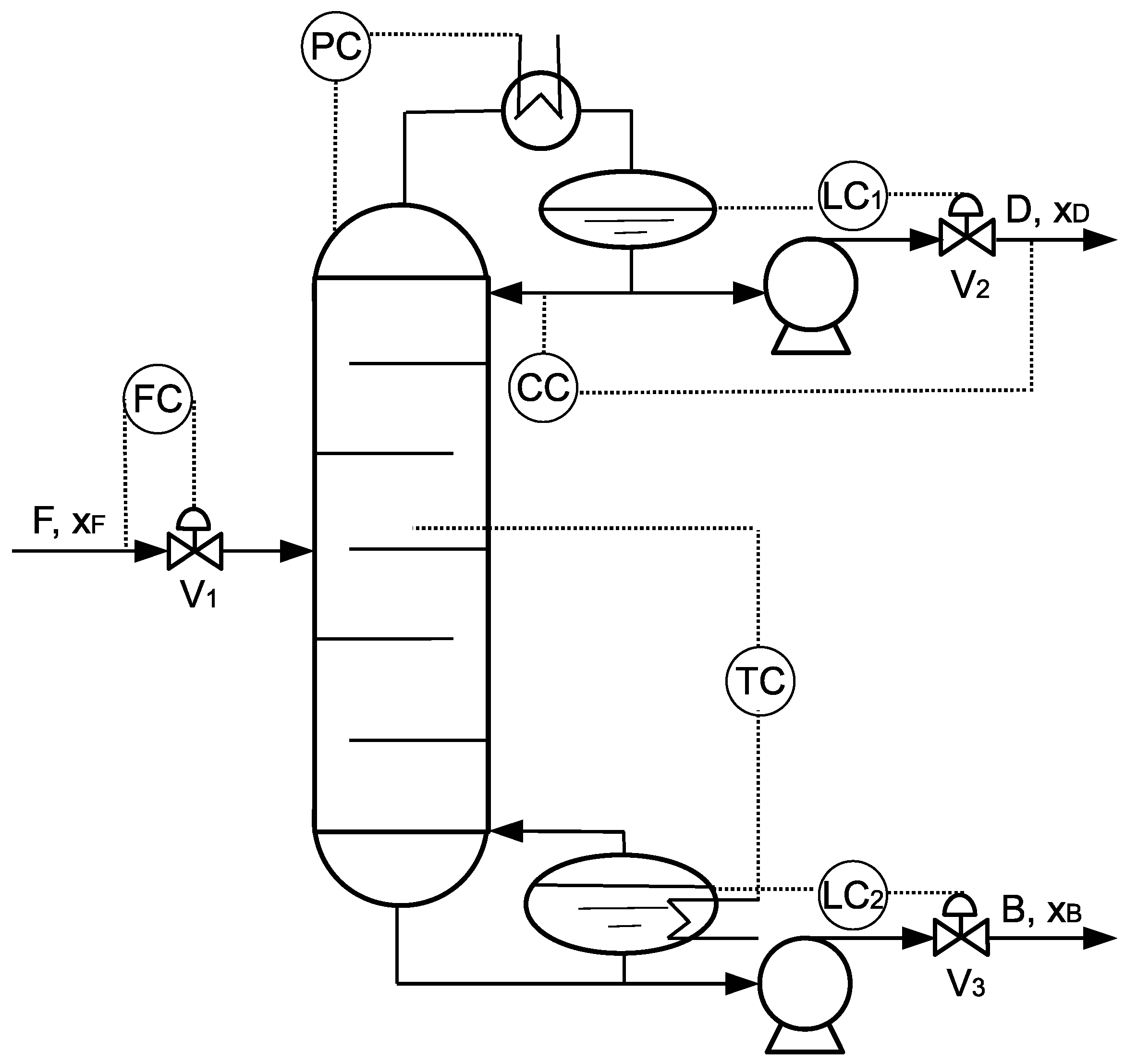
Six controllers were added in the distillation column, four of which had fixed set-points and two of which received set-points from RTO. The control scheme is shown in Figure 12.

(1) A flow rate controller $FC$ is controlling the feed mole flow rate at 1 kmol/s by manipulating feed valve $V_1$. A fixed feed flow rate helps to fix the parameters in the first-principles steady-state model.

(2) A pressure controller $PC$ is controlling the column top pressure at 16.8 atm by manipulating condenser heat duty $Q_{top}$. A fixed column pressure helps to operate the process with fixed thermodynamic properties.

(3) A level controller $L{C}_1$ is controlling the reflux drum liquid level at 5.1 m by manipulating the distillate outlet valve $V_2$. A certain liquid level in the condenser is required to avoid flooding or drying.

(4) A level controller $L{C}_2$ is controlling the reboiler liquid level at 6.35 m by manipulating the bottom outlet valve $V_3$. A certain liquid level in the reboiler is required to avoid flooding or drying.

(5) A concentration controller $CC$ is controlling the distillate $C_3$ mole fraction by manipulating the reflux mole flow rate. A time delay of 5 min was added to simulate the concentration measurement delay. At the beginning of each RTO period, RTO sends the optimized distillate $C_3$ mole fraction $x_D$ to concentration controller $CC$ as the set-point. Then, controller $CC$ adjusts the reflux flow to track the mole fraction to its set-point.

(6) A temperature controller $TC$ is controlling temperature $T_7$ on Tray 7, by manipulating reboiler heat duty $Q_{bottom}$. A time delay of 1 min was added to simulate the temperature measurement delay. Tray temperature control is common in industry, and two methods were carried out to determine the best tray temperature to be controlled. A steady-state simulation was used to obtain the temperature profile along the tube to find out that the temperature changes among Tray 6, Tray 7, and Tray 8 were greater than those among other trays. One more simulation was performed to get the gain of tray temperature as a response to a small change in the reboiler heat duty. It was also found that the temperature on Tray 7 had a greater gain than those on other trays. As a result, Tray 7 was chosen as the controlled variable.

At the beginning of the RTO period, RTO optimizes the profit and calculates a set of steady-states. Given the optimum value of R, D, B, $x_D$,$x_B$, the steady-state model of $F_1=0$, $F_2=0$, and $F_3=0$ were used again to obtain the concentration profile in the distillation column. Then, the neural network model $T_n=F_{NN,2}\left(y_n\right)$ was used to calculate the temperature on Tray 7. After that, the tray temperature $T_7$ was sent to the controller $TC$ and will be tracked to its set-point by manipulating the reboiler heat duty.

Flow rate controller $FC$, pressure controller $PC$, and both level controllers $L{C}_1$ and $L{C}_2$ had fixed set-points, which stabilized the process to operate at fixed operation parameters. Concentration controller $CC$ and temperature controller $TC$ received set-points from RTO at the beginning of RTO period and drove the process to more profitable steady-state. All the PI parameters were tuned by the Ziegler–Nichols method and are shown in

Table 3. Proportional gain and integral time constant of all the PI controllers in the distillation case study.

	KC	τI/min
FC	0.5	0.3
PC	15	12
LC1	2	150
LC2	4	150
CC	0.1	20
TC	0.6	8

.

4.4. Simulation Results

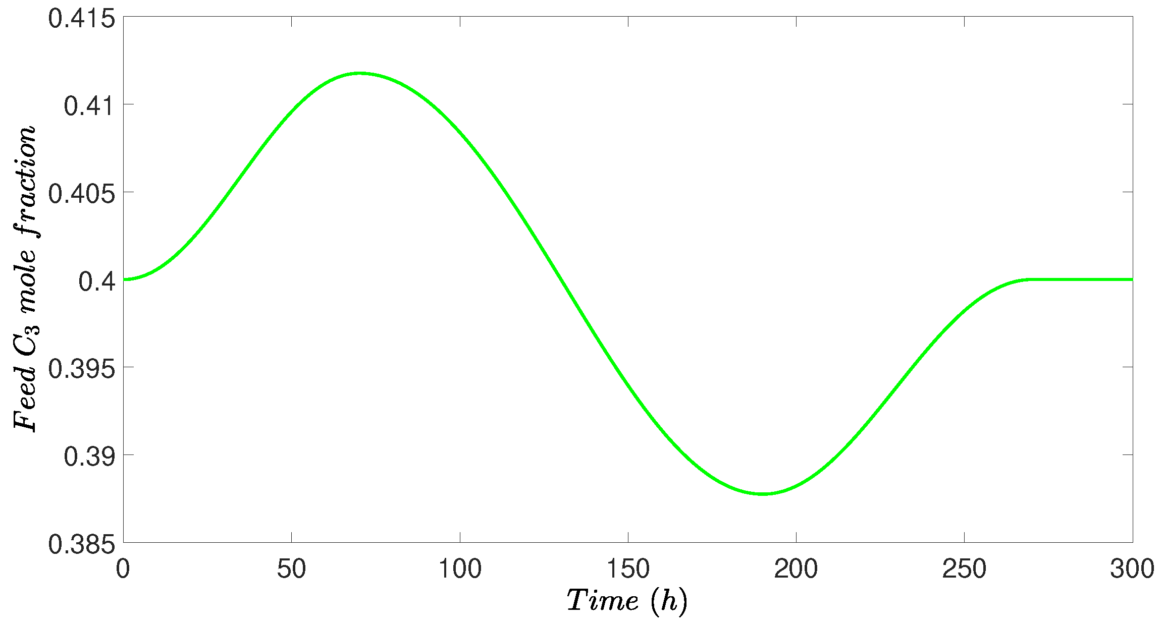
To demonstrate the effectiveness of RTO, a variation in feed mole fraction $x_F$ was introduced to the process, as shown in Figure 13. At the beginning of each RTO period (20 h), one measurement of feed mole fraction $x_F$ was sent to RTO to optimize the profit. Then, a set of steady-states was achieved from RTO and was sent to the controllers as set-points.

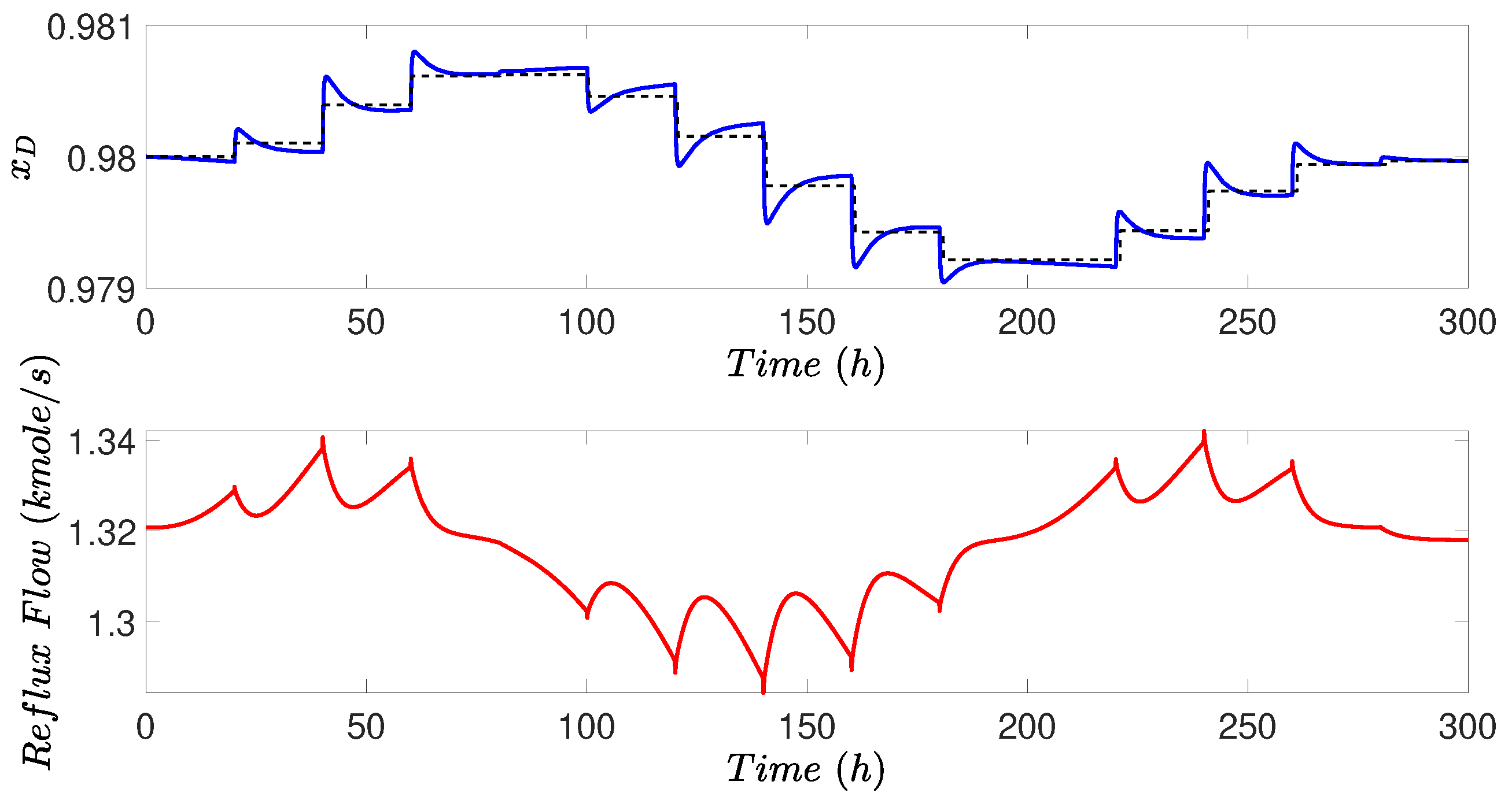
The simulation results are shown in Figure 14 and Figure 15. In Figure 14, the set-point of $x_D$ increases as feed concentration $x_F$ increases at the beginning of simulation, because higher distillate concentration is more profitable and more feed concentration $x_F$ allows further separation to achieve a higher concentration in the distillate. The set-point for $x_D$ also decreased later when feed concentration $x_F$ decreased. At the beginning of the simulation, reflux flow increased to reach higher $x_D$ set-points, and reflux flow never reached a steady-state during the whole simulation because the feed component kept changing as shown in Figure 13. In some cases, the mole fraction $x_D$ did not track exactly the set-point because of the ever-changing feed, too small set-point change, and coupled effect with other variables and controllers.

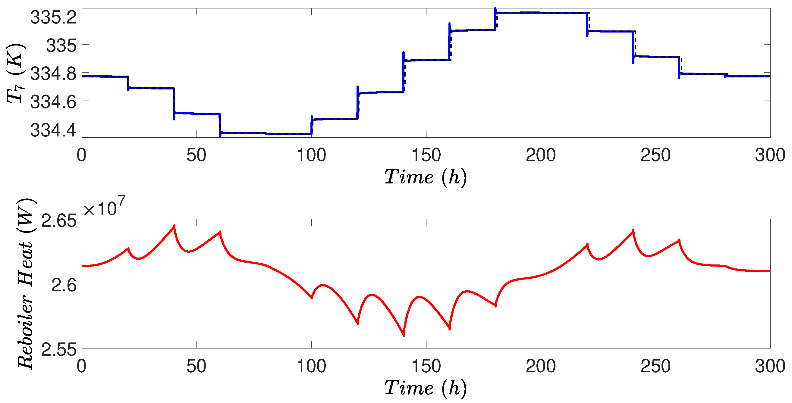
Figure 15 illustrates the performance of temperature controller $TC$. When the feed $x_F$ increased, the set-point for Tray 7 temperature $T_7$ decreased according to RTO. The controller then manipulated the reboiler heat duty to track the tray temperature with a good performance as shown in Figure 15. It is noted in Figure 15 that the reboiler heat duty increased as tray temperature decreased at the beginning of the simulation. The reason is that the reboiler heat duty mainly dependent on the liquid flow into the reboiler and the vapor flow leaving the reboiler. Since the reflux flow was increased by the concentration controller $CC$ at the beginning of simulation, both the liquid flow into the reboiler and vapor leaving the reboiler increased, thus increasing reboiler heat duty.

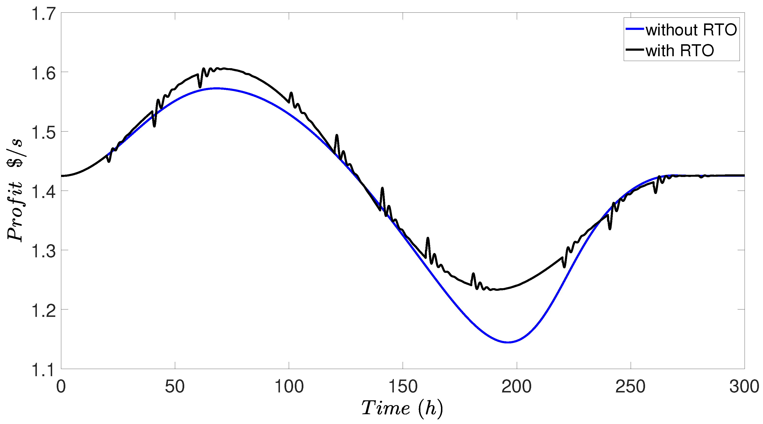
Other controllers stayed at the fixed set-points throughout the simulation by adjusting their manipulated inputs. Therefore, we are not showing the plots for other controllers. It is demonstrated in Figure 16 that the RTO increased the operation profit when distillation column had a varying feed concentration. The profit in Figure 16 was calculated by the profit definition of Equation (20), using the closed-loop simulation data for variables D, B, F, and R. The black line is the operation profit calculated by the closed-loop simulation where the four controllers ($FC$, $PC$, $L{C}_1$, and $L{C}_2$) had fixed set-points and the two controllers ($CC$ and $TC$) had varying set-points from RTO. The blue line is the simulation where the set-points of all controllers were fixed at the initial steady-state and the controlled variables stayed at the initial set-point by adjusting manipulated variables in the presence of the same feed variation in Figure 13. Although the feed concentration kept changing each second and RTO updated the steady-state only each 20 h, the profit was still improved significantly by RTO, as shown in Figure 16.

In this case study, a neural network model was combined only with the steady-state first-principles model, not the dynamic model. Additionally, it was demonstrated that the steady-states calculated by RTO using a combination of models were very close to the steady-state values in the Aspen simulator, which means that the combination of the neural network model and first-principles model was of high accuracy. The neural network model was used to represent the phase equilibrium properties for RTO to calculate the optimal steady-state in this work. Neural network models can be useful when the phase equilibrium is highly nonlinear such that the first-principles model is inaccurate. Additionally, it can be used when a large number of states are included in thermodynamic equations, such as pressure or more concentrations for the multi-component case.

5. Conclusions

In this work, we presented a method for integrating neural network modeling with first-principles modeling in the model used in RTO and MPC. First, a general framework that integrates neural network models with first-principle models in the optimization problems of RTO and MPC was discussed. Then, two chemical process examples were studied in this work. In the first case study, a CSTR with reversible exothermic reaction was utilized to analyze the performance of integrating the neural network model and first-principles model in RTO and MPC. Specifically, a neural network was first built to represent the nonlinear reaction rate. An RTO was designed to find the operating steady-state providing the optimal balance between the energy cost and reactant conversion. Then, an LMPC was designed to stabilize the process to the optimal operating condition. A variation in energy price was introduced, and the simulation results demonstrated that RTO minimized the operation cost and yielded a closed-loop performance that was very close to the one attained by RTO/MPC using the first-principles model. In the second case study, a distillation column was studied to demonstrate an application to a large-scale chemical process. A neural network was first trained to obtain the phase equilibrium properties. An RTO scheme was designed to maximize the operation profit and calculate the optimal set-points for the controllers using a neural network model with a first-principles model. A variation in the feed concentration was introduced to demonstrate that RTO increased operation profit for all considered conditions. In closing, it is important to note that the two simulation studies only demonstrated how the proposed approach can be applied and provided some type of “proof of concept” on the use of hybrid models in RTO and MPC, but certainly, both examples yield limited conclusions and cannot substitute for an industrial/experimental implementation to evaluate the proposed approach, which would be the subject of future work.

References

- Bhutani, N.; Rangaiah, G.; Ray, A. First-principles, data-based, and hybrid modeling and optimization of an industrial hydrocracking unit. Ind. Eng. Chem. Res. 2006, 45, 7807–7816. [Google Scholar] [CrossRef]
- Pantelides, C.C.; Renfro, J. The online use of first-principles models in process operations: Review, current status and future needs. Comput. Chem. Eng. 2013, 51, 136–148. [Google Scholar] [CrossRef]
- Quelhas, A.D.; de Jesus, N.J.C.; Pinto, J.C. Common vulnerabilities of RTO implementations in real chemical processes. Can. J. Chem. Eng. 2013, 91, 652–668. [Google Scholar] [CrossRef]
- Wu, Z.; Tran, A.; Rincon, D.; Christofides, P.D. Machine Learning-Based Predictive Control of Nonlinear Processes. Part I: Theory. AIChE J. 2019, 65, e16729. [Google Scholar] [CrossRef]
- Wu, Z.; Tran, A.; Rincon, D.; Christofides, P.D. Machine Learning-Based Predictive Control of Nonlinear Processes. Part II: Computational Implementation. AIChE J. 2019, 65, e16734. [Google Scholar] [CrossRef]
- Lee, M.; Park, S. A new scheme combining neural feedforward control with model-predictive control. AIChE J. 1992, 38, 193–200. [Google Scholar] [CrossRef]
- Venkatasubramanian, V. The promise of artificial intelligence in chemical engineering: Is it here, finally? AIChE J. 2019, 65, 466–478. [Google Scholar] [CrossRef]
- Himmelblau, D. Applications of artificial neural networks in chemical engineering. Korean J. Chem. Eng. 2000, 17, 373–392. [Google Scholar] [CrossRef]
- Chouai, A.; Laugier, S.; Richon, D. Modeling of thermodynamic properties using neural networks: Application to refrigerants. Fluid Phase Equilib. 2002, 199, 53–62. [Google Scholar] [CrossRef]
- Galván, I.M.; Zaldívar, J.M.; Hernandez, H.; Molga, E. The use of neural networks for fitting complex kinetic data. Comput. Chem. Eng. 1996, 20, 1451–1465. [Google Scholar] [CrossRef] [Green Version]
- Faúndez, C.A.; Quiero, F.A.; Valderrama, J. Phase equilibrium modeling in ethanol+ congener mixtures using an artificial neural network. Fluid Phase Equilib. 2010, 292, 29–35. [Google Scholar] [CrossRef]
- Fu, K.; Chen, G.; Sema, T.; Zhang, X.; Liang, Z.; Idem, R.; Tontiwachwuthikul, P. Experimental study on mass transfer and prediction using artificial neural network for CO2 absorption into aqueous DETA. Chem. Eng. Sci. 2013, 100, 195–202. [Google Scholar] [CrossRef]
- Bakshi, B.; Koulouris, A.; Stephanopoulos, G. Wave-Nets: Novel learning techniques, and the induction of physically interpretable models. In Wavelet Applications; International Society for Optics and Photonics: Orlando, FL, USA, 1994; Volume 2242, pp. 637–648. [Google Scholar]
- Lu, Y.; Rajora, M.; Zou, P.; Liang, S. Physics-embedded machine learning: Case study with electrochemical micro-machining. Machines 2017, 5, 4. [Google Scholar] [CrossRef]
- Psichogios, D.C.; Ungar, L.H. A hybrid neural network-first principles approach to process modeling. AIChE J. 1992, 38, 1499–1511. [Google Scholar] [CrossRef]
- Oliveira, R. Combining first principles modelling and artificial neural networks: A general framework. Comput. Chem. Eng. 2004, 28, 755–766. [Google Scholar] [CrossRef]
- Chen, L.; Bernard, O.; Bastin, G.; Angelov, P. Hybrid modelling of biotechnological processes using neural networks. Control Eng. Pract. 2000, 8, 821–827. [Google Scholar] [CrossRef]
- Georgieva, P.; Meireles, M.; de Azevedo, S. Knowledge-based hybrid modelling of a batch crystallisation when accounting for nucleation, growth and agglomeration phenomena. Chem. Eng. Sci. 2003, 58, 3699–3713. [Google Scholar] [CrossRef]
- Schuppert, A.; Mrziglod, T. Hybrid Model Identification and Discrimination with Practical Examples from the Chemical Industry. In Hybrid Modeling in Process Industries; CRC Press: Boca Raton, FL, USA, 2018; pp. 63–88. [Google Scholar]
- Qin, S.; Badgwell, T. A survey of industrial model predictive control technology. Control Eng. Pract. 2003, 11, 733–764. [Google Scholar] [CrossRef]
- Câmara, M.; Quelhas, A.; Pinto, J. Performance evaluation of real industrial RTO systems. Processes 2016, 4, 44–64. [Google Scholar] [CrossRef]
- Lee, W.J.; Na, J.; Kim, K.; Lee, C.; Lee, Y.; Lee, J.M. NARX modeling for real-time optimization of air and gas compression systems in chemical processes. Comput. Chem. Eng. 2018, 115, 262–274. [Google Scholar] [CrossRef]
- Agbi, C.; Song, Z.; Krogh, B. Parameter identifiability for multi-zone building models. In Proceedings of the 2012 IEEE 51st IEEE Conference on Decision and Control (CDC), Maui, HI, USA, 10–13 December 2012; pp. 6951–6956. [Google Scholar]
- Yen-Di Tsen, A.; Jang, S.S.; Wong, D.S.H.; Joseph, B. Predictive control of quality in batch polymerization using hybrid ANN models. AIChE J. 1996, 42, 455–465. [Google Scholar] [CrossRef]
- Klimasauskas, C.C. Hybrid modeling for robust nonlinear multivariable control. ISA Trans. 1998, 37, 291–297. [Google Scholar] [CrossRef]
- Chang, J.; Lu, S.; Chiu, Y. Dynamic modeling of batch polymerization reactors via the hybrid neural-network rate-function approach. Chem. Eng. J. 2007, 130, 19–28. [Google Scholar] [CrossRef]
- Noor, R.M.; Ahmad, Z.; Don, M.M.; Uzir, M.H. Modelling and control of different types of polymerization processes using neural networks technique: A review. Can. J. Chem. Eng. 2010, 88, 1065–1084. [Google Scholar] [CrossRef]
- Wang, J.; Cao, L.L.; Wu, H.Y.; Li, X.G.; Jin, Q.B. Dynamic modeling and optimal control of batch reactors, based on structure approaching hybrid neural networks. Ind. Eng. Chem. Res. 2011, 50, 6174–6186. [Google Scholar] [CrossRef]
- Chaffart, D.; Ricardez-Sandoval, L.A. Optimization and control of a thin film growth process: A hybrid first principles/artificial neural network based multiscale modelling approach. Comput. Chem. Eng. 2018, 119, 465–479. [Google Scholar] [CrossRef]
- Schweidtmann, A.M.; Mitsos, A. Deterministic global optimization with artificial neural networks embedded. J. Opt. Theory Appl. 2019, 180, 925–948. [Google Scholar] [CrossRef]
- Wu, Z.; Christofides, P.D. Economic Machine-Learning-Based Predictive Control of Nonlinear Systems. Mathematics 2019, 7, 494. [Google Scholar] [CrossRef]
- Goodfellow, I.; Bengio, Y.; Courville, A. Deep Learning; MIT Press: Cambridge, MA, USA, 2016. [Google Scholar]
- Bishop, C. Pattern Recognition and Machine Learning; Springer: New York, NY, USA, 2006. [Google Scholar]
- Haykin, S. Neural Networks: A Comprehensive Foundation; Prentice Hall PTR: Upper Saddle River, NJ, USA, 1994. [Google Scholar]
- Naysmith, M.; Douglas, P. Review of real time optimization in the chemical process industries. Dev. Chem. Eng. Miner. Process. 1995, 3, 67–87. [Google Scholar] [CrossRef]
- Rawlings, J.; Amrit, R. Optimizing process economic performance using model predictive control. In Nonlinear Model Predictive Control; Springer: Berlin, Germany, 2009; pp. 19–138. [Google Scholar]
- Ellis, M.; Durand, H.; Christofides, P. A tutorial review of economic model predictive control methods. J. Process Control 2014, 24, 1156–1178. [Google Scholar] [CrossRef]
- Rawlings, J.B.; Bonné, D.; Jørgensen, J.B.; Venkat, A.N.; Jørgensen, S.B. Unreachable setpoints in model predictive control. IEEE Transa. Autom. Control 2008, 53, 2209–2215. [Google Scholar] [CrossRef]
- Mhaskar, P.; El-Farra, N.H.; Christofides, P.D. Stabilization of nonlinear systems with state and control constraints using Lyapunov-based predictive control. Syst. Control Lett. 2006, 55, 650–659. [Google Scholar] [CrossRef]
- Wang, L. Continuous time model predictive control design using orthonormal functions. Int. J. Control 2001, 74, 1588–1600. [Google Scholar] [CrossRef]
- Hosseinzadeh, M.; Cotorruelo, A.; Limon, D.; Garone, E. Constrained Control of Linear Systems Subject to Combinations of Intersections and Unions of Concave Constraints. IEEE Control Syst. Lett. 2019, 3, 571–576. [Google Scholar] [CrossRef]
- Daoutidis, P.; Kravaris, C. Dynamic output feedback control of minimum-phase multivariable nonlinear processes. Chem. Eng. Sci. 1994, 49, 433–447. [Google Scholar] [CrossRef] [Green Version]
- Economou, C.; Morari, M.; Palsson, B. Internal model control: Extension to nonlinear system. Ind. Eng. Chem. Process Des. Dev. 1986, 25, 403–411. [Google Scholar] [CrossRef]
- Lin, Y.; Sontag, E. A universal formula for stabilization with bounded controls. Syst. Control Lett. 1991, 16, 393–397. [Google Scholar] [CrossRef]
- Luyben, W.L. Distillation Design and Control Using Aspen Simulation; John Wiley & Sons: Hoboken, NJ, USA, 2013. [Google Scholar]
- Al-Malah, K.I. Aspen Plus: Chemical Engineering Applications; John Wiley & Sons: Hoboken, NJ, USA, 2016. [Google Scholar]
- Aspen Technology, Inc. Aspen Plus User Guide; Aspen Technology, Inc.: Cambridge, MA, USA, 2003. [Google Scholar]
Figure 1.
A feed-forward neural network with input , hidden neurons , and outputs . Each weight is marked on the structure. Neuron “1” is used to represent the biases.
Figure 2.
Steady-state profiles ( and T) for the CSTR of Equation (8) under varying heat input rate Q, where the minimum of is achieved at Q = 59,983 cal/s.
Figure 3.
Error distribution histogram for training, validation, and testing data.
Figure 4.
Heat price profile during the simulation, where the heat price first increases and then decreases to simulate heat rate price changing.
Figure 5.
Evolution of the concentration of A and B for the CSTR case study under the proposed real-time optimization (RTO) and MPC.
Figure 6.
Evolution of the reactor temperature T for the CSTR case study under the proposed RTO and MPC scheme.
Figure 7.
Evolution of the manipulated input, the heating rate Q, for the CSTR example under the proposed RTO and MPC scheme.
Figure 8.
Comparison of the total operation cost for the CSTR example for simulations with and without RTO adapting to the heat rate price changing.
Figure 9.
A schematic diagram of the distillation column implemented in Aspen Plus Dynamics.
Figure 10.
Comparison of the neural network model and the Aspen model.
Figure 11.
Figure 12.
A schematic diagram of the control structure implemented in the distillation column. Flow rate controller , pressure controller , and both level controllers and have fixed set-points, and concentration controller and temperature controller receive set-points from the RTO.
Figure 13.
The feed concentration profile of the distillation column, which is changing with respect to time.
Figure 14.
Controlled output and manipulated input for the concentration controller in the distillation process under the proposed RTO scheme.
Figure 15.
Controlled output and manipulated input for the temperature controller in the distillation process under the proposed RTO scheme.
Figure 16.
Comparison of the operation profit for the distillation process for closed-loop simulations with and without RTO adapting for change in the feed concentration.