An Optimisation-Driven Prediction Method for Automated Diagnosis and Prognosis

Abstract

This article presents a novel hybrid classification paradigm for medical diagnoses and prognoses prediction. The core mechanism of the proposed method relies on a centroid classification algorithm whose logic is exploited to formulate the classification task as a real-valued optimisation problem. A novel metaheuristic combining the algorithmic structure of Swarm Intelligence optimisers with the probabilistic search models of Estimation of Distribution Algorithms is designed to optimise such a problem, thus leading to high-accuracy predictions. This method is tested over 11 medical datasets and compared against 14 cherry-picked classification algorithms. Results show that the proposed approach is competitive and superior to the state-of-the-art on several occasions.

1. Introduction

Artificial Intelligence (AI) plays a major role in modern medicine and is key in automating tasks such as image registration [1,2,3], diagnosis [4,5] and prognosis [6,7], thus allowing for doctors and practitioners to make faster and more accurate decisions [8]. Indeed, recent advances in AI have made it possible for expert systems [9] and machine learning techniques [1,10] to outperform human decision-making over some repetitive procedures and are definitely more accurate at spotting hidden patterns in medical images or signals. Obviously, this does not mean that human intervention can be completely removed, in particular in the medical diagnosis domain, but the latter can significantly benefit from the informative feedback returned by AI-based diagnoses and prognosis systems. For instance, convolutional neural networks can be fed with EGG signals or magnetic resonance imaging (MRI) images to predict diagnoses of neurodegenerative diseases, for example Alzheimer’s [11,12], and accurately classify brain lesions [13,14,15]. In this light, applied AI displays a valuable societal impact and carries a promising potential for improving upon decision-making in medicine. However, the use of computer-aided diagnosis is sometimes criticised and despite the medical community being aware of the importance of modernising its methods, some researchers are hesitant due to the possibility of false-positive or false-negative cases, and some others point out moral implications [16]. This stimulates and motivates computer scientists, who continually search for new and more accurate techniques. Room for improvement is easily identified for example, in the context of historical data analysis. Large databases are nowadays available and can be used without the need for ethical approval. Hence, exploiting this knowledge optimally for training AI techniques would help generate more reliable automatic diagnosis and prognosis predictions.

To achieve this goal, supervised machine-learning is currently preferred in medicine [10], as data are labelled based on the kind of tissue, prognosis, patient age and several other useful features, to perform prediction. Successful studies using supervised classification strategies, for example., cardiovascular medicine [17] and genetics [18], are present in the literature. However, better performances can be obtained by optimising the classification process. For this reason, this piece of research proposes a novel classification method, referred to as “Optimisation-Driven Prediction” (ODP), to be used for automated medical diagnosis and prognosis. This classifier is designed around a newly designed variant of a metaheuristic for real-valued optimisation, referred to as Particle Swarm Estimation of Distribution Algorithm (PSEDA), originally proposed in Reference [19].

The remainder of this article is structured as follows:

• Section 2 gives a brief overview of the metaheuristics optimisation approaches employed in this study and highlights differences between previous classification schemes based on optimisation algorithms and the proposed method;
• Section 3 clarifies objectives and methods for this piece of research;
• Section 4 describes the proposed ODP method, including an explanation of the working principle behind the novel PSEDA variant, the definition of the classification process in the fashion of an optimisation problem and the formulation of five different objective functions, aka fitness function, to strengthen the validity of the proposed approach;
• Section 5 gives details of the experimental phase to make the presented results reproducible;
• Section 6 presents and discuss the numerical results;
• Section 7 concludes this work by summarising the key research outputs and drawing some considerations for possible future developments.

2. Background and Related Work

Particle Swarm Optimization (PSO) [20] is the most popular Swarm Intelligence (SI) metaheuristic [21,22,23] for solving numerical optimization problems. Similar to common population-based Evolutionary Algorithms (EAs) [24], it employs a set of candidate solutions to first explore the search space to then converge to the most promising basin of attraction. On the other hand, the PSO lacks selection mechanisms, which are usually replaced with the 1-to-1 spawning mechanisms in SI algorithms and features a unique perturbation strategy mimicking starling flocks’ behaviour. Hence, solutions move and interact, rather than being evolved as in EAs, according to the dynamics outlined in Reference [25]. Several PSO variants have been designed to deal with a wide range of problems [26], including large scale ones [27,28], as well as challenging engineering applications [29], and hybrid versions were also designed thus generating effective PSO based multi-strategy approaches [30] and Estimation of Distribution Algorithms (EDAs) [31,32]. The EDA framework is quite interesting and has proven to be successful over different fields such as Robotics [33] and combinatorial domains [21]. These algorithms have a probabilistic representation of the population, thus are not required to store individuals since they are sampled on-demand from distribution of probabilities. The latter is continually adapted to the problem at hand so that sampled candidate solutions have a higher probability of falling in a neighbourhood of the optimal solution. Some examples of EDAs, referred to as “compact” algorithms, can be found in Reference [32]. It is also worth mentioning the so-called BOA-PSO algorithm, proposed in Reference [34], where a multivariate distribution is used instead of a set of univariate distributions (i.e., one per design variable), the EDPSO algorithm designed in Reference [35], which uses a mixture of univariate Gaussian distributions, as well as the more recent variant in Reference [36], where an EDA is used to model the “historical memory” of successful solutions in a PSO framework. Similarly, the Particle Swarm Estimation of Distribution Algorithm (PSEDA) introduced in Reference [19] is based on adjusting a probability distribution to simulate the behaviour of a classic PSO. PSEDA has proven to be efficient and to outperform classic PSO algorithms over several optimisation problems. In this light, the PSEDA framework was further improved in this piece of research and then used in the proposed ODP approach.

It must be said that the literature already presents classification methods using metaheuristic for numerical optimisation but these differ from ODP. As an example, a genetic algorithm is used in Reference [37] for finding optimal coefficients of a wavelet kernel extreme learning classifier, while a memetic algorithm is used in Reference [38] to optimise a model for gene selection in microarray data. Moreover, past studies made use of a standard PSO in Reference [39] as well as the Artificial Bee Colony paradigm (ABC) [40] for data classification and clustering, respectively. Conversely, in the ODP method optimisation is used at the training level. The PSEDA variant described in Section 4.1, and schematically shown in Algorithm 1, is embedded in ODP and used to automatically tailor a classifier to the dataset.

3. Objectives and Methods

This research intends to design a novel prediction method for medical diagnosis and prognosis capable of classifying multivariate healthcare datasets with high accuracy and, therefore, a low rate of false negatives and positives.

In light of what was described in Section 2, the PSEDA algorithm was chosen for its outstanding performances [19] and for its algorithmic features, which make it behaves similarly to SI algorithms, as the PSO successfully used for the classification problem in Reference [39], and EDAs (which are a kind of EAs), simultaneously. Technical details on the working mechanisms of PSEDA are given in Section 4.1. To further improve upon the classification process, the PSEDA algorithm was not simply employed but was improved by introducing a self-adaptive mechanism to adjust the exploratory step-size on-the-fly. By using this novel variant, referred to as self-adaptive PSEDA (sa–PSEDA), the proposed method always returns optimal, or near-optimal, predictions. Indications on how to use sa–PSEDA for classification purposes are in Section 4.2.

In a nutshell, the proposed methodology consists of defining the classification process in the form of an optimisation problem, which requires the formulation of an objective function, aka a fitness function, within the metaheuristic optimisation community. To perform a thorough comparative analysis and give more validity to our results, five different fitness functions are considered in this study. Three of them are cherry-picked from the literature [39], while two more are originally proposed for this specific piece of research. A rigorous analytical formulation of the employed fitness function is given in Section 4.2.

Finally, the methodology for evaluating the performances of sa–PSEDA consists of using 11 different multivariate medical datasets from the “UCI machine learning repository” [41] and generating predictions with each fitness function. To perform a fair comparison, classification results are also produced with the previously mentioned PSO and ABC methods from References [39,40]. Their implementation is made available in an online repository reachable from https://bit.ly/2VK9CS3. Moreover, a comparison against popular classifiers, that is, a naive nearest centroid classifier, and 11 more state-of-the-art methods in their Weka [42] implementation, is also carried out. The statistical tests in Reference [42] are used to validate the comparative analysis and draw rigorous conclusions.

4. The Optimisation-Driven Prediction Method

The ODP method is a supervised classification approach requiring training data to generate a prediction function. To perform the training process optimally, a metaheuristic for continuous optimisation is used. This means that the classification task must be formulated as an optimisation problem. This process requires the definition of at least a fitness functions, a formal description of the search space and an appropriate encoding strategy to represent class representatives as candidate solutions. These details are clarified in the following sections.

4.1. The sa–PSEDA Algorithm

The original PSEDA in Reference [19] simulates the internal dynamics of a PSO algorithm with a probabilistic model. Unlike other EDAs, this is achieved by associating each “particle” with its own probabilistic model. The latter are update and moved in the search space according to the PSO logic, which requires attractors as the local (i.e., a neighboured of a particle must be considered) and the global (i.e., in the entire swarm is considered) best solutions, to then sample a new particle in a different location of the search space. Hence, these distributions are used instead of the so-called “velocity” vector, which is the PSO perturbation vector added to the particles to move them towards most promising regions. Advantages of having a stochastic perturbation are evident over multimodal problems and reduce the rise of deleterious structural biases [25,43,44].

Without loss of generality, let us suppose to have a generic minimisation problem in the domain $\Theta ={[l_k,u_k]}^d\subseteq {\mathbb{R}}^d$ ($k=1,2,3,\cdots ,d$) where a real valued fitness function $f:\Theta \to \mathbb{R}$ is defined. The ith particle in the PSEDA’s swarm ($i=1,2,3,\cdots ,\mathrm{NP}$), at generic iteration t, is associated with the following d-dimensional vectors:

• position $x_{i,t}\in \Theta$;
• personal best position $p_{i,t}=\underset{s\le t}{argmin}f(x_{i,s})$;
• global best $g_t=\underset{1\le i\le n}{argmin}f(p_{i,t})$;
• position, personal best, and global best at the previous generation, that is, $x_{i,t-1}$, $p_{i,t-1}$, and $g_{t-1}$ respectively.

During an iteration cycle of PSEDA, the joint probability distribution ${\mathcal{P}}_{i,t}$ of each $x_{i,t}$ vector is updated to then produce $x_{i,t+1}\sim {\mathcal{P}}_{i,t}$. This is done on the assumption that the d components of each position vector can be modelled with independent and identically distributed (iid) random variables. Under this condition, ${\mathcal{P}}_{i,t}$ can be factorised in d unidimensional probability density functions

$${\mathcal{P}}_{i,t}=\prod _{k=1}^d{\mathcal{P}}_{i,t,k}$$

which facilitates the implementation of the algorithm and leads to a modest algorithmic time overhead, since each kth component can be efficiently sampled from $x_{i,t+1,k}\sim {\mathcal{P}}_{i,t,k}$. Each iid variable is modelled via a weighted finite mixture [45] of the following probability distributions:

• ${\mathcal{TN}}_{i,t,k}^{(x)}$, that is, a truncated (within $[l_k,u_k]$) normal distribution with mean value $x_{i,t,k}$ and standard deviation ${\sigma }_{i,t,k}^{(x)}$;
• ${\mathcal{TN}}_{i,t,k}^{(p)}$, that is, a truncated (within $[l_k,u_k]$) normal distribution with mean value $p_{i,t,k}$ and standard deviation ${\sigma }_{i,t,k}^{(p)}$;
• ${\mathcal{TN}}_{t,k}^{(g)}$, that is, a truncated (within $[l_k,u_k]$) normal distribution with mean value $g_{t,k}$ and standard deviation ${\sigma }_{t,k}^{(g)}$;
• ${\mathcal{U}}_k$, that is, a uniform distribution within $[l_k,u_k]$;
• ${\overline{\mathcal{P}}}_{i,t-1,k}$, that is, a relaxed variant of the mixture ${\mathcal{P}}_{i,t-1,k}$ composed by the three truncated normal distributions ${\mathcal{TN}}_{i,t-1,k}^{(x)}$, ${\mathcal{TN}}_{i,t-1,k}^{(p)}$, ${\mathcal{TN}}_{t-1,k}^{(g)}$ of the previous iteration cycle $t-1$.

It must be noted that the use of truncated distributions prevents the algorithm from generating infeasible solutions and thus removes the need for correction strategies [44]. The distributions are weighted with $w_x$, $w_p$, $w_g$, $w_u$ and $w_m$ as described in Reference [19]. Then, the mechanism in Reference [45] is employed to sample a candidate solution. This requires the roulette wheel tournament scheme (see e.g., Reference [24]) as also described in Reference [19].

It is worth observing that the truncated normal distributions are centered on the particle, its personal best particle and global best particle, in order to mimic the PSO working logic. Since points surrounding the mean value of a normal distribution have a higher probability of being selected, by narrowing the standard deviation PSEDA becomes almost identical to a PSO. On the other hand, higher standard deviation values result in different algorithmic behaviours. In light of this, it is obvious that convergence speed also depends on the standard deviation values of the normal distributions. To make sure that these values are self-adapted on the problem at hand during the optimisation process, the proposed sa–PSEDA variant is equipped with the tuning mechanism, formalised with the equations below:

$${\sigma }_{i,t,k}^{(x)}\leftarrow \left\{\begin{array}{cc}min\left\{\right|x_{i,t,k}-p_{i,t,k}|,|x_{i,t,k}-g_{t,k}\left|\right\}\hfill & \mathrm{if} \mathrm{it} \mathrm{is} \mathrm{greater} \mathrm{than} 0\hfill \\ {ϵ}_{i,t,k}^{(x)}\hfill & \mathrm{otherwise}\hfill \end{array}\right.$$

(1)

$${\sigma }_{i,t,k}^{(p)}\leftarrow \left\{\begin{array}{cc}min\left\{\right|p_{i,t,k}-x_{i,t,k}|,|p_{i,t,k}-g_{t,k}\left|\right\}\hfill & \mathrm{if} \mathrm{it} \mathrm{is} \mathrm{greater} \mathrm{than} 0\hfill \\ {ϵ}_{i,t,k}^{(p)}\hfill & \mathrm{otherwise}\hfill \end{array}\right.$$

(2)

$${\sigma }_{t,k}^{(g)}\leftarrow \left\{\begin{array}{cc}min\left\{\right|g_{t,k}-x_{i,t,k}|,|g_{t,k}-p_{i,t,k}\left|\right\}\hfill & \mathrm{if} \mathrm{it} \mathrm{is} \mathrm{greater} \mathrm{than} 0\hfill \\ {ϵ}_{i,t,k}^{(g)}\hfill & \mathrm{otherwise}\hfill \end{array}\right.$$

(3)

where ${ϵ}_{i,t,k}^{(x)}$, ${ϵ}_{i,t,k}^{(p)}$, ${ϵ}_{i,t,k}^{(g)}$ are small random numbers uniformly distributed in $[0,0.01]$. The starting value for each standard deviation is the smaller distance between the peak of the truncated normal distribution and the peak of the remaining truncated normal distributions.

Algorithm 1 sa–PSEDA

1: proceduresa–PSEDA 2:   $t\leftarrow 0$ 3:   Randomly initialize the n individuals 4:   while $t<M$ do       ▹M is the number of allowed generations 5:    for all individuals ($i=1,dots,\mathrm{NP}$) do 6:     Evaluate fitness $f(x_{i,t})$ 7:     Save the previous personal best $p_{i,t-1}$ 8:     Update personal best $p_{i,t}$ 9:    end for 10:    Save the previous global best $g_{t-1}$ 11:    Update global best $g_t$ 12:    for all individuals i do 13:     for all dimensions k do 14:      Compute ${\sigma }_{i,t,k}^{(x)}$, ${\sigma }_{i,t,k}^{(p)}$, ${\sigma }_{t,k}^{(g)}$ according to Equations (1)–(3) 15:      Save the previous position $x_{i,t-1}$ 16:      Sample $x_{i,t+1,k}$ from $P_{i,t,k}$    ▹ with the method in [45] 17:     end for 18:    end for 19:    $t\leftarrow t+1$ 20:   end while 21: end procedure

Finally, it is also worth noting that the distribution $\overline{\mathcal{P}}$ was designed to reproduce the effect of the velocity vector, while the uniform distribution ${\mathcal{U}}_k$ was introduced in order to regulate the exploration/exploitation balance of the evolutionary search [46].

For the sake of clarity, the sa–PSEDA algorithmic framework is shown in the pseudo-code in Algorithm 1.

4.2. The Classification Strategy

Classification is a classic application of machine learning [47] consisting of generating a prediction from labelled observations. In this work, such observations are numerical values. This format is quite common in health care data as the vast majority of medical tests return values that are then labelled by finding the range of belonging.

Formally, this format can be expressed by defining instances with real-valued vectors of the kind $A\subseteq {\mathbb{R}}^m$ and the class space for the classification problem as an ordered set $B=\{1,\cdots ,k\}$ of integers values. The classification process takes place via two main sequential phases—(1) the training of a prediction function $h:A\to B$ over a training set $T=\left\{(a_i,b_i)|a_i\in A,b_i\in B\right\}$; (2) the use of the fine-tuned prediction function over new datasets.

Typical methods for implementing the prediction function h are decision trees [48], aggregations or associations rules [49,50], a Bayesian or neural network [51] or hybrid approaches such as, for example, fuzzy neural systems [52]. However, in this work, we preferred the centroid algorithm from Reference [53]. This was already used in SI classifiers in the past [39,40] and requires the computation of the centroid for each class, which is not a computationally expensive procedure (i.e., it does not introduce overheads in the ODP method) and it is suitable for real-value datasets.

A formal definition of the adopted prediction function is

$$h_{x^{(1)},\cdots ,x^{(k)}}(a)=\underset{1\le i\le k}{argmin}d(x^{(i)},a)$$

(4)

where $x^{(i)}\in A$ is the centroid of the class $i\in B$, and $d(·,·)$ is the Euclidean distance. Since $A\subseteq {\mathbb{R}}^m$ and $\left|B\right|=k$, the use of $h_{x^{(1)},\cdots ,x^{(k)}}$ comes with an acceptable computational complexity (i.e., $O\left(k·m\right)$).

The proposed sa-PSEDA can now be used to “train” h by finding its optimal parameters, that is, the class representatives $x^{(1)},\cdots ,x^{(k)}$. This means that the prediction function is actually “evolved” and tailored to the specific classification task, which is now stated as an optimisation problem. The sa-PSEDA is then a key component of the classifier, operating in a search space $\Theta \subseteq {\mathbb{R}}^{k·m}$ where candidate solutions $x\in \Theta$ are represented in the form $x=\langle x^{(1)},\cdots ,x^{(k)}\rangle$ with $x^{(i)}\in {\mathbb{R}}^m$ and $i\in \{1,\cdots ,k\}$) since each one of the k classes has m numerical features.

In order to evaluate the quality of a generic solution x on the training set T, five different fitness functions have been taken into account:

$${\psi }_1(x)=\frac{1}{\left|T\right|}\sum _{(a_i,b_i)\in T}\delta (x,a_i,b_i)$$

(5)

$${\psi }_2(x)=\frac{1}{\left|T\right|}\sum _{(a_i,b_i)\in T}\overline{d}(a_i,x^{(b_i)})$$

(6)

$${\psi }_3(x)=0.50·{\psi }_1(x)+0.50·{\psi }_2(x)$$

(7)

$${\psi }_4(x)=0.25·{\psi }_1(x)+0.75·{\psi }_2(x)$$

(8)

$${\psi }_5(x)=0.75·{\psi }_1(x)+0.25·{\psi }_2(x)$$

(9)

where $\overline{d}:{\mathbb{R}}^m\times {\mathbb{R}}^m\to [0,1]$ is the normalised Euclidean distance, introduced in Reference [39], while

$$\delta (x,a_i,b_i)=\left\{\begin{array}{cc}1\hfill & \mathrm{if}{h}_{x^{(1)},\cdots ,x^{(k)}}(a_i)\ne b_i\hfill \\ 0\hfill & \mathrm{otherwise}\hfill \end{array}\right.$$

By minimising the proposed fitness functions the same optimisation algorithm can be used to perform five different training processes. To distinguish between them, the fitness function is added to the algorithm’s name as follows: sa–PSEDA-${\psi }_1$, sa–PSEDA-${\psi }_2$, sa–PSEDA-${\psi }_3$, sa–PSEDA-${\psi }_4$, and sa–PSEDA-${\psi }_5$.

It must be remarked that the first three fitness functions have been proposed in previous studies [39,40], while the remaining two are originally designed to perform a wider comparative analysis. The ${\psi }_1$ function represents the error rate on the training set and has a complexity of $O(|T|·k·m)$, while ${\psi }_2$ computes the average distance of training instances from the class representative of the known classes. The latter comes with a lower complexity of $O(|T|·m)$ but not necessarily with an inferior quality of the results. ${\psi }_3$, ${\psi }_4$, ${\psi }_5$ are convex combinations of the first two fitness functions and only differ by the adopted weights (i.e., ${\psi }_3$ is balanced with equal weights while ${\psi }_4$ and ${\psi }_5$ are unbalanced toward ${\psi }_1$ and ${\psi }_2$ respectively). The last three fitness functions have the same complexity of ${\psi }_1$ and are obtained by composing ${\psi }_1$ and ${\psi }_2$.

5. Experimental Setup

The ODP method was run over 11 well-known medical datasets for diagnosis and prognosis, taken from the UCI machine learning repository [41], and evaluated with 10 repetitions of the stratified 10-folds cross-validation technique. During each repetition, the dataset is split into 10 batches, each one following the same class distribution of the entire dataset. Then, instances from 9 batches are used to train the supervised classifier while the 10th batch is used for testing the learned model. In total, 100 test rounds are performed for every dataset, thus the performances of every algorithm are averaged over the 100 tests and the corresponding results are provided in Section 6.

A detailed description of the 11 employed datasets is given in Section 5.1. Moreover, it must be stressed out that the presented results are obtained by using sa–PSEDA with the parameter setting reported in Section 5.2, where comparison algorithms are also listed. These values for the parameters are the outcomes of a fine-tuning empirical process carried out to train the classifier optimally.

5.1. The Datasets

The 11 classification datasets are described in

Table 1. Test problems.

Dataset	#Inst.	#Classes	#Attr.	#Real	#Int.	#Log.	Missing Inf.
Breast-Real	569	2	30	30	0	0	no
Breast-Integer	699	2	9	0	9	0	yes
Dermatology	366	6	34	0	33	1	yes
Diabetes	768	2	8	2	6	0	no
Haberman	306	2	3	0	3	0	no
Heart-2C	303	2	13	1	9	3	yes
Heart-5C	303	5	13	1	9	3	yes
Liver	341	2	6	1	5	0	no
Parkinsons	195	2	22	22	0	0	no
Thyroid	215	3	5	4	1	0	no
Vertebral	310	3	6	6	0	0	no

, which schematically shows the number of instances, class labels, attributes, the attributes’ structure (i.e., the number of real-valued, integer, and logical attributes) and a warning to flag missing information. Indeed, it is quite common to find datasets with missing information in medicine. However, this problem can be easily dealt with as data are numerical and missing fields can be replaced with the average value of the present values [40].

From Table 1 it can be easily noticed that the chosen problems are diverse and are adequate to test the versatility of the proposed method. Moreover, each dataset has a multivariate nature and presents strong dependencies amongst the attributes. For the sake of completeness, a concise description of each dataset is given below.

Breast-Real and Breast-Integer are based on the “Breast Cancer Wisconsin (Diagnostic)” and “Breast Cancer Wisconsin (Original)” datasets from UCI. In this article, instances are classified in two diagnosis class, that is, benign and malign breast cancer, respectively. Both the datasets come with an ID field that was removed to perform our experiments. It must be noted that, while the first dataset is real-valued, the second one has integer attributes in the range $[1,10]$. However, this is not an issue as the ODP method can indifferently work on real-valued sets and its subsets.

Dermatology contains diagnoses of erythematous-squamous diseases and is the largest dataset considered in this study with its 33 integer attributes, in the range $[0,3]$, and 1 logical attribute (i.e., Boolean) per instance. The six possible diagnoses are—Psoriasis, Seborrheic Dermatitis, Lichen Planus, Pityriasis Rosea, Chronic dermatitis, and Pityriasis Rubra Pilaris.

Diabetes is based on the “Pima Indians Diabetes” dataset for diabetes diagnoses of female patients. It has six integer attributes, each with a large cardinality, and two real-valued attributes.

Haberman is a database of long-term survivors who undergone breast surgeries and provides information on the survival time, for example, whether or not the patient died within 5 years from the surgery. It represents the smaller dataset considered in this study in terms of the number of attributes. The latter are three integer values with a large cardinality.

Heart-2C and Heart-5C contain data from heart disease diagnoses from the “Cleveland Processed Heart Disease” dataset in UCI. The difference between the two datasets is in the number of classes. Heart-2C can be used as a binary classification problem (i.e., the patient is diseased or not), while Heart-5C has four possible classes defined by specific vascular parameters. These two datasets have one real-valued, logical and integer attributes.

Liver is a database of liver disorders, mainly due to excessive alcohol consumption, in male patients. Attributes have both real-valued and integer formats and refer to blood test results. One must be aware that this dataset contains duplicated instances that need to be removed before being used. This issue is pointed out in the UCI website.

Parkinsons consists of a range of biomedical voice measurements from healthy individuals and patients affected by Parkinson’s disease. This dataset was downloaded from the UCI repository and the field containing the patient’s name was removed from each attribute as not relevant to this study.

Thyroid is based on the “new-thyroid” dataset from UCI and contains diagnoses of thyroid gland diseases. It has three classes—normal, hyperthyroidism and hypothyroidism.

Vertebral, aka “Vertebral Column” dataset, contains values for six biomechanical features used to classify orthopaedic patients into the three “normal,” “disk hernia” and “spondylolisthesis” classes. Also in this case, the dataset is multivariate.

5.2. Parameter Settings and Comparison Algorithms

The suggested parameters configuration for the sa–PSEDA predecessor in Reference [19] indicates a swarm size of 50 particles and variation operator’s parameters equal to $\omega =0.7298$ and ${\phi }_1={\phi }_2=1.49618$ respectively. This leads to the calculation of the $w_x$, $w_p$ and $w_g$ weights, discussed in Section 4.1, as shown below:

• $w_x=w_m=(1-w_u)·0.5·\frac{\omega }{\omega +{\phi }_1+{\phi }_2}$;
• $w_p=(1-w_u)·\frac{{\phi }_1}{\omega +{\phi }_1+{\phi }_2}$;
• $w_g=(1-w_u)·\frac{{\phi }_2}{\omega +{\phi }_1+{\phi }_2}$;

while $w_u$ was set to $0.05$.

These values were tested with the sa–PSEDA variant and compared against several other parameters combinations. We concluded that the same setting can be used for sa–PSEDA apart from the value for the $w_u$ weight. The latter has to be lowered down to $0.01$ to obtain optimal performances. This conclusion was obtained by running sa-PSEDA with a computational budget fixed to 300,000 fitness evaluations over four common testbed problems:

• Schwefel 1.2:

  $$f(x_1,x_2,\cdots ,x_d)=\sum _{i=1}^d{\left(\sum _{j=1}^i{x}_j\right)}^2$$

  where $-100\le x_i\le 100$, $x^{\ast }=0,0,\cdots ,0$ and $f_{min}(x^{\ast })=0$;
• Rosenbrock:

  $$f(x_1,x_2,\cdots ,x_d)=\sum _{i=1}^{d-1}\left[100{\left(x_{i+1}-x_i^2\right)}^2+{\left(x_i-1\right)}^2\right]$$

  where $-10\le x_i\le 10$, $x^{\ast }=1,1,\cdots ,1$ and $f_{min}(x^{\ast })=0$;
• Rastrigin:

  $$f(x_1,x_2,\cdots ,x_d)=An+\sum _{i=1}^n\left[x_i^2-10cos(2\pi x_i)\right]$$

  where $-5.12\le x_i\le 5.12$, $x^{\ast }=0,0,\cdots ,0$ and $f_{min}(x^{\ast })=0$;
• Ackley:

  $$f(x_1,x_2,\cdots ,x_d)=-20e^{-0.2\sqrt{\frac{1}{d}{\displaystyle \sum _{i=1}^d}{x}_i^2}}-e^{\frac{1}{d}{\displaystyle \sum _{i=1}^d}cos\left(2\pi x_i\right)}+20+e$$

  where $-32.768\le x_i\le 32.768$, $x^{\ast }=0,0,\cdots ,0$ and $f_{min}(x^{\ast })=0$;

displaying different fitness landscapes. Further details and source code (implemented in Java) for these functions can be found in [54]. This experiment was repeated 50 times per problem to observe the average performances and its standard deviation. Each problem was considered at $d=30$ and $d=10$ dimension values.

Table 2. Tuning results on numerical benchmarks.

Benchmark	d	Minimum Fitness (avg ± std)		Statistical Difference
		sa-PSEDA ${\mathit{w}}_{\mathit{u}}=0.01$	sa-PSEDA ${\mathit{w}}_{\mathit{u}}=0.05$
Schwefel 1.2	30	$\mathbf{0}\pm 0$	$2.1127\pm 1.6295$	no
	10	$\mathbf{0}\pm 0$	$\mathbf{0}\pm 0$	no
Rosenbrock	30	$\mathbf{8.9764}\pm 13.2544$	$47.3852\pm 34.5774$	yes
	10	$\mathbf{0.0315}\pm 0.0475$	$0.2110\pm 0.3535$	no
Rastrigin	30	$\mathbf{0}\pm 0$	$0.0200\pm 0.1393$	yes
	10	$\mathbf{0}\pm 0$	$\mathbf{0}\pm 0$	no
Ackley	30	$\mathbf{0}\pm 0$	$\mathbf{0}\pm 0$	no
	10	$\mathbf{0}\pm 0$	$\mathbf{0}\pm 0$	no

shows a comparison obtained by executing sa–PSEDA with $w_u$ equal to $0.05$ (as proposed in the [19]) and $0.01$. The best results, displayed in boldface, show that $0.01$ is preferable. This is also confirmed with the t-test outcome reported, with a compact yes/no notation, in the last column of Table 2. In this column, a “yes” indicates that the variant with $w_u=0.01$ statistically outperforms the other variant, while a “no” means that the two variants are statistically equivalent.

It can be noted that sa-PSEDA seems to be very robust and resilient to variations of parameters as results are very similar. Hover, since improvements are registered with $w_u=0.01$, this value was used instead of the one proposed for PSEDA in Reference [19].

To show the quality of the proposed ODP method, when equipped with the fine-tuned sa–PSEDA optimiser, a set of comparison algorithms was chosen from the literature, as explained in Section 3.

Thus, the classification approach using a PSO algorithm in Reference [39] was implemented and run over the 11 datasets used in this study with the parameter settings proposed by its authors, namely $n=50$, $T_{max}=1000$, $v_{max}=0.05$, $v_{min}=-0.05$, $c_1=2.0$, $c_2=2.0$, $w_{max}=0.9$ and $w_{min}=0.4$.

Moreover, the classification approach using the ABC algorithm in Reference [40] was also implemented and run with the parameter settings proposed by its authors, namely a colony size of 20, a maximum generations number of 2500 and a limit value of 1000. To perform a fair comparison, the proposed number of iterations for the PSO was increased from 1000 to 2500 in order to obtain the same number of fitness evaluations (i.e., 50,000) used for sa–PSEDA and PSO over the 11 classification problems.

The source codes used for sa–PSEDA, PSO and ABC are made available in an online repository reachable from https://bit.ly/2VK9CS3.

Finally, 12 popular classification methods were selected. The first one is the Nearest-Centroid (NC) classifier used, for example, in References [53,55]. This classifier was taken into consideration as similar to the classification mechanism of the proposed ODP method, even though it does not come with an effective training logic. Usually, this kind of method is employed when a very fast classification process is required. The other 11 classification strategies are instead state-of-the-art schemes taken from the Weka software suite (release 3.8) [42]. Weka contains a large number of Bayesian, functions-based, lazy (or instance-based), meta-schemes, rules-based, tree-based and so on, classifiers. We have chosen some methods from each available group to have a wider range of classification techniques. These are:

• the Bayes Net in Reference [56];
• the Multi Layer Perceptron Artificial Neural Network (MLP) in Reference [57];
• the Radial Basis Function Artificial Neural Network (RBF) in Reference [58];
• the Nearest Neighbor (NN) method in Reference [59];
• the k-Nearest Neighbors (kNN) in Reference [59] with $k=5$;
• the lazy “k-Star” scheme in Reference [60];
• the Bagging method in Reference [61];
• the MultiBoostAB (MBAB) algorithm in Reference [62];
• the Ripple Down Rule learner (Ridor) [63];
• the popular Naive Bayes classifier (NBTree) [64];
• the Voting Feature Intervals classifier (VFI) proposed in Reference [65].

Unless differently specified in the list above, all these methods were run with the parameter settings indicated in the original articles.

Considering that five instances of sa–PSEDA, PSO and ABC have been executed—that is, one per fitness function—a total of 27 classification schemes were run in this investigation. All the classifiers based on optimisation algorithm are referred with the same notation of ODP, that is, sa–PSEDA-${\psi }_i$, PSO-${\psi }_i$ and ABC-${\psi }_i$ where $i=1,2,3,4,5$ is the number of the fitness function listed in Section 4.2.

6. Experimental Results

Due to a large number of results being obtained with the 27 classifiers and the 10 repetitions of the 10-folds cross-validation method, which means that 2700 classification tasks were run, results are arranged in two groups. Section 6.1 contains the comparison amongst the three classifiers using SI metaheuristics for optimisation plus the NC method. In Section 6.2 the best amongst the five sa–PSEDA instances (individuated in Section 6.1) were compared against the 11 state-of-the-art algorithms from Weka.

Numerical results are displayed in tables in terms of average accuracy (±standard deviation). The best value is highlighted in boldface. The outcome of the test of significance returned by the Weka platform [42] is also reported (i.e., a paired t-test with confidence level set to $0.05$) to validate results statistically. A compact notation is used. The equals sign = indicates the comparisons which results are statistically equivalent, that is, the distribution of the results of the reference algorithm does not significantly differ from the distribution of the comparison algorithm, while circles are used to point out significant statistical differences. In particular, a black circle • refers to the case where the reference algorithm outperforms the comparison algorithm. Conversely, a white one ○ indicates that the reference algorithm is outperformed by the comparison algorithm.

6.1. Comparison against SI Classifiers

In total, 15 SI classifiers are evaluated.

Table 3. Average accuracy ± standard deviation and statistical analysis [42] for the 15 SI classifiers and the NC classifier over the 11 classification problems.

Algorithm	Avg Accuracy	Statistical Analysis
sa-PSEDA-${\psi }_1$	81.45 ± 13.61	−
PSO-${\psi }_1$	80.35 ± 13.39	$2•$ $9=$ $0○$
ABC-${\psi }_1$	80.53 ± 13.30	$3•$ $7=$ $1○$
sa-PSEDA-${\psi }_2$	77.40 ± 16.59	−
PSO-${\psi }_2$	76.59 ± 15.96	$1•$ $10=$ $0○$
ABC-${\psi }_2$	77.48 ± 16.69	$0•$ $10=$ $1○$
sa-PSEDA-${\psi }_3$	82.90 ± 13.70	−
PSO-${\psi }_3$	82.66 ± 13.75	$3•$ $7=$ $1○$
ABC-${\psi }_3$	82.07 ± 13.85	$5•$ $6=$ $0○$
sa-PSEDA-${\psi }_4$	82.23 ± 14.16	−
PSO-${\psi }_4$	81.90 ± 14.09	$2•$ $8=$ $1○$
ABC-${\psi }_4$	81.87 ± 14.06	$3•$ $8=$ $0○$
sa-PSEDA-${\psi }_5$	82.92 ± 13.88	−
PSO-${\psi }_5$	82.51 ± 14.02	$2•$ $9=$ $0○$
ABC-${\psi }_5$	81.91 ± 13.91	$6•$ $5=$ $0○$
NC	78.15 ± 16.13	$10•$ $0=$ $1○$

compares their classification performances by arranging the three main methods into five groups according to the employed fitness function, that is, ${\psi }_1$ and $ps{i}_2$${\psi }_3$ and ${\psi }_4$ and ${\psi }_5$. The reference algorithm of each ith group ($i=1,2,3,4,5$) is sa–PSEDA-${\psi }_i$. It must be remarked that the NC classifier, which does not use the SI logic, is also added here as the ODP method contains a similar classifier (trained with sa–PSEDA). Thus, it is appropriate to include it in this comparison.

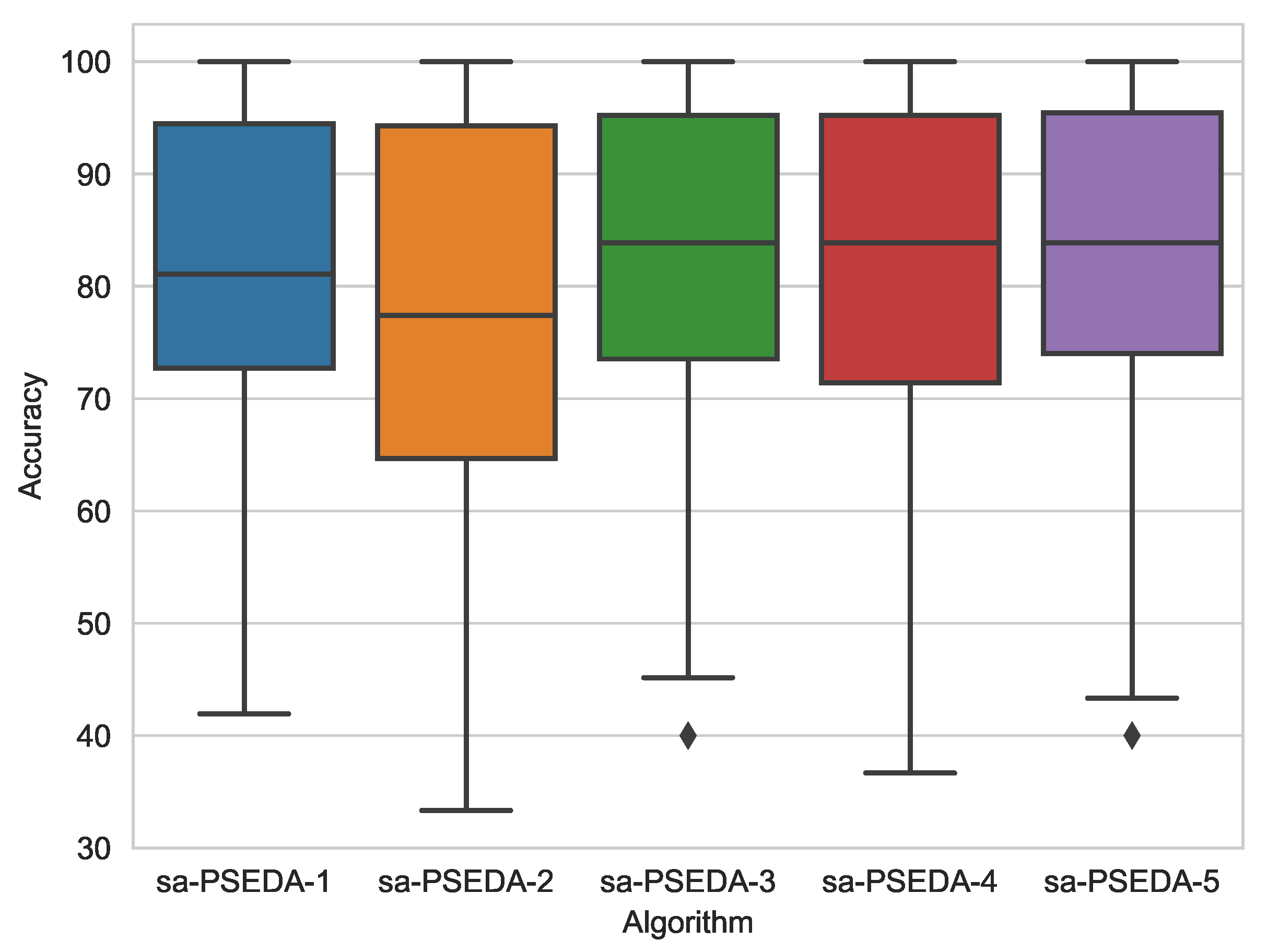
It can be noted that sa–PSEDA displays the overall best performance. However, it is interesting to observe that when ${\psi }_2$ is employed, the ABC based classier obtains the best performance and statistically outperform sa–PSEDA in one case (it is equivalent to sa–PSEDA otherwise). Conversely, if the other fitness functions are used, sa–PSEDA always displays the best average result and it outperforms the other methods also statistically. This means that the second fitness function is not suitable for modelling the problems at hands, as it is the only one deteriorating the performances of the proposed method. The best accuracy is obtained by employing ${\psi }_5$, as highlighted in the box plot in Figure 1 and the statistical analysis in

Table 4. Average accuracy ± standard deviation and statistical analysis [42] for sa-PSEDA-${\psi }_5$ against sa-PSEDA-${\psi }_1$,sa-PSEDA-${\psi }_2$, sa-PSEDA-${\psi }_3$ and sa-PSEDA-${\psi }_4$ over the 11 classification problems.

Algorithm	Avg Accuracy	Statistical Analysis
sa-PSEDA-${\psi }_1$	81.45 ± 13.61	$7•$ $4=$ $0○$
sa-PSEDA-${\psi }_2$	77.40 ± 16.59	$10•$ $1=$ $0○$
sa-PSEDA-${\psi }_3$	82.90 ± 13.70	$1•$ $10=$ $0○$
sa-PSEDA-${\psi }_4$	82.23 ± 14.16	$6•$ $4=$ $1○$
sa-PSEDA-${\psi }_5$	82.92 ± 13.88	−

.

The comparison between the NC method and sa–PSEDA-${\psi }_5$ shows that ODP always outperforms its predecessor (i.e., NC). This motivates the proposed ODP method, which is basically an optimised version of the NC classifier. In this light, this work shows that extremely complex classification strategies are not necessary, as a simple one can be enhanced by optimising the training process (as done in ODP). This is even more evident in Section 6.2, where state-of-the-art classifiers are compared against the ODP method.

It also worth spending a few words on the key role played by the fitness function. Recently, the research community has been producing novel bio-inspired metaheursitcs for optimisation in an attempt to obtain better results. However, most of the novel algorithms share very similar structures, as, for example, firefly algorithms [66] and differential evolution [44,67] are ruled by similar internal dynamics [25] and are designed without taking into consideration the problem at hand. This process does not always lead to optimal results, as it is known that universal optimisers do not exist, and the best performance is always returned by algorithms tailored to the problem [68]. In this light, more attention should be paid to the formulation of the problem by defining an informative fitness function. For these reasons, the five functions used in this paper were defined to provide a variety of fitness landscapes and different results were expected depending on their use.

To summarise, the classifiers returning the first, second and third best accuracy value over each problem are listed in

Table 5. Best Swarm Intelligence (SI) classification methods (plus nearest centroid (NC)).

Dataset	Best Classifier	2nd Best Classifier	3rd Best Classifier
Breast-Real	PSO-${\psi }_5$	sa–PSEDA-${\mathbf{\psi }}_{\mathbf{5}}$	sa–PSEDA-${\psi }_3$
Breast-Integer	sa–PSEDA-${\mathbf{\psi }}_{\mathbf{5}}$	PSO-${\psi }_5$	PSO-${\psi }_3$
Dermatology	ABC-${\psi }_2$	sa–PSEDA-${\psi }_4$	NC
Diabetes	sa–PSEDA-${\psi }_1$	sa–PSEDA-${\mathbf{\psi }}_{\mathbf{5}}$	sa–PSEDA-${\psi }_3$
Haberman	ABC-${\psi }_5$	sa–PSEDA-${\mathbf{\psi }}_{\mathbf{5}}$	PSO-${\psi }_5$
Heart-2C	PSO-${\psi }_4$	sa–PSEDA-${\psi }_3$	PSO-${\psi }_3$
Heart-5C	sa–PSEDA-${\psi }_3$	PSO-${\psi }_1$	sa–PSEDA-${\mathbf{\psi }}_{\mathbf{5}}$
Liver	PSO-${\psi }_3$	sa–PSEDA-${\mathbf{\psi }}_{\mathbf{5}}$	PSO-${\psi }_5$
Parkinsons	sa–PSEDA-${\psi }_1$	sa–PSEDA-${\mathbf{\psi }}_{\mathbf{5}}$	sa–PSEDA-${\psi }_3$
Thyroid	PSO-${\psi }_5$	sa–PSEDA-${\mathbf{\psi }}_{\mathbf{5}}$	sa–PSEDA-${\psi }_3$
Vertebral	PSO-${\psi }_5$	sa–PSEDA-${\mathbf{\psi }}_{\mathbf{5}}$	PSO-${\psi }_5$
All	sa–PSEDA-${\mathbf{\psi }}_{\mathbf{5}}$	sa–PSEDA-${\psi }_3$	PSO-${\psi }_3$

. This table gives a better overview and further confirms the superiority of sa-PSEDA-${\psi }_5$ and sa–PSEDA in general. Indeed, the second-best classification approach is sa–PSEDA-${\psi }_3$ and the only two datasets where sa–PSEDA is not listed amongst the first three most effective classifiers are Dermatology and Heart-2C.

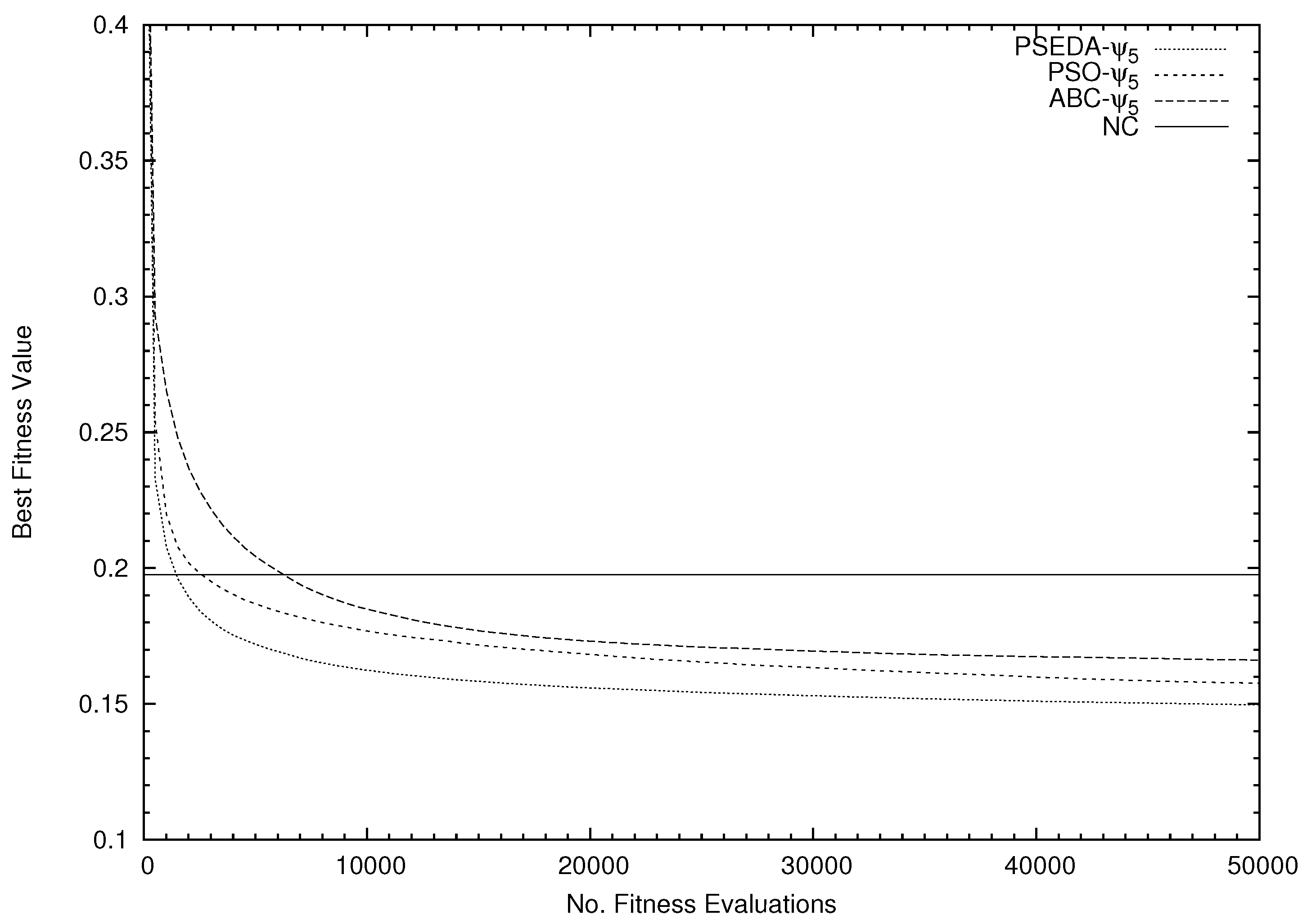
An explanation of the poor performance obtained over the Dermatology dataset in comparison with that one obtained with the simple NC method can be related to an inadequate computational budget of the sa–PSEDA algorithm. Indeed, this dataset has 204 (6 classes × 34 attributes) and might require more fitness functional calls, while the NC method is not affected by this problem. This should be investigated, as PSO and ABC perform better despite using the same computational budget, even though sa–PSEDA-${\psi }_5$ has the overall (i.e., average) fastest convergence speed, as shown in Figure 2.

Finally, it can be observed that using a combination of ${\psi }_1$ and ${\psi }_2$ leads to better results only if higher importance is given to ${\psi }_1$. This is what is done in function ${\psi }_5$. Conversely, unbalancing the weights towards ${\psi }_1$, as done in ${\psi }_4$, is not beneficial as the obtained classification carry an accuracy inferior to the one of ${\psi }_3$ (which is balanced).

6.2. Comparison against State-of-the-Art Classifiers

A thorough comparative analysis is performed in

Table 6. Average accuracy ± standard deviation and statistical analysis [42] for sa-PSEDA-${\psi }_5$ against state-of-the-art algorithms from Reference [42] over the 11 classification problems.

Dataset	sa–PSEDA-${\mathit{\psi }}_5$	BayesNet		MLP		RBF		NN		kNN		kStar		Bagging		MBAB		Ridor		NBTree		VFI
Breast-Real	$\mathbf{97.08}$	$94.40$	$•$	$96.61$	$•$	$94.22$	$•$	$95.64$	$•$	$96.88$		$94.66$	$•$	$94.87$	$•$	$93.55$	$•$	$93.91$	$•$	$93.89$	$•$	$91.37$	$•$
	$(\pm 2.22)$	$(\pm 3.29)$		$(\pm 2.45)$		$(\pm 3.15)$		$(\pm 2.32)$		$(\pm 2.25)$		$(\pm 2.76)$		$(\pm 2.99)$		$(\pm 3.88)$		$(\pm 3.41)$		$(\pm 3.16)$		$(\pm 3.00)$
Breast-Integer	$96.88$	$\mathbf{97.20}$	$○$	$95.65$	$•$	$96.09$	$•$	$95.34$	$•$	$96.94$		$95.35$	$•$	$95.50$	$•$	$94.34$	$•$	$95.32$	$•$	$96.31$	$•$	$95.62$	$•$
	$(\pm 2.13)$	$(\pm 1.70)$		$(\pm 2.50)$		$(\pm 2.22)$		$(\pm 2.59)$		$(\pm 1.99)$		$(\pm 2.54)$		$(\pm 2.59)$		$(\pm 3.11)$		$(\pm 2.52)$		$(\pm 2.29)$		$(\pm 2.62)$
Dermatology	$95.55$	$\mathbf{97.98}$	$○$	$97.34$	$○$	$96.29$		$95.60$		$96.91$	$○$	$94.56$	$•$	$96.42$	$○$	$50.27$	$•$	$95.20$		$96.33$		$91.50$	$•$
	$(\pm 3.31)$	$(\pm 2.38)$		$(\pm 2.47)$		$(\pm 2.83)$		$(\pm 3.16)$		$(\pm 2.56)$		$(\pm 3.55)$		$(\pm 2.94)$		$(\pm 1.12)$		$(\pm 3.72)$		$(\pm 3.26)$		$(\pm 3.90)$
Diabetes	$\mathbf{76.55}$	$75.25$	$•$	$74.75$	$•$	$74.04$	$•$	$70.62$	$•$	$73.86$	$•$	$70.19$	$•$	$75.42$	$•$	$73.38$	$•$	$72.97$	$•$	$75.24$	$•$	$62.57$	$•$
	$(\pm 4.56)$	$(\pm 4.78)$		$(\pm 4.90)$		$(\pm 4.91)$		$(\pm 4.67)$		$(\pm 4.61)$		$(\pm 4.77)$		$(\pm 4.62)$		$(\pm 5.74)$		$(\pm 4.78)$		$(\pm 5.23)$		$(\pm 5.35)$
Haberman	$\mathbf{75.60}$	$71.57$	$•$	$73.87$	$•$	$73.79$	$•$	$66.03$	$•$	$70.49$	$•$	$70.27$	$•$	$73.56$	$•$	$72.79$	$•$	$72.52$	$•$	$71.94$	$•$	$57.83$	$•$
	$(\pm 6.95)$	$(\pm 3.95)$		$(\pm 6.27)$		$(\pm 5.16)$		$(\pm 6.66)$		$(\pm 5.17)$		$(\pm 5.80)$		$(\pm 5.64)$		$(\pm 5.75)$		$(\pm 5.79)$		$(\pm 4.53)$		$(\pm 11.31)$
Heart-2C	$\mathbf{82.81}$	$82.63$		$79.48$	$•$	$82.30$		$75.48$	$•$	$80.57$	$•$	$74.64$	$•$	$81.88$		$82.05$		$77.23$	$•$	$79.87$	$•$	$78.73$	$•$
	$(\pm 7.57)$	$(\pm 7.78)$		$(\pm 7.80)$		$(\pm 7.40)$		$(\pm 8.03)$		$(\pm 7.33)$		$(\pm 7.62)$		$(\pm 7.67)$		$(\pm 7.64)$		$(\pm 8.25)$		$(\pm 7.02)$		$(\pm 8.07)$
Heart-5C	$56.67$	$\mathbf{56.85}$		$53.02$	$•$	$56.58$		$52.94$	$•$	$55.70$		$50.33$	$•$	$57.94$		$51.89$	$•$	$54.71$	$•$	$53.69$	$•$	$42.99$	$•$
	$(\pm 7.07)$	$(\pm 6.66)$		$(\pm 7.49)$		$(\pm 7.42)$		$(\pm 6.55)$		$(\pm 6.54)$		$(\pm 6.02)$		$(\pm 4.91)$		$(\pm 5.04)$		$(\pm 6.20)$		$(\pm 5.95)$		$(\pm 7.82)$
Liver	$68.88$	$56.58$	$•$	$69.00$		$65.61$	$•$	$61.86$	$•$	$61.56$	$•$	$65.93$	$•$	$\mathbf{70.21}$		$64.88$	$•$	$66.11$	$•$	$64.49$	$•$	$59.22$	$•$
	$(\pm 7.09)$	$(\pm 4.44)$		$(\pm 8.07)$		$(\pm 7.51)$		$(\pm 7.20)$		$(\pm 8.56)$		$(\pm 7.65)$		$(\pm 6.92)$		$(\pm 7.24)$		$(\pm 6.54)$		$(\pm 6.93)$		$(\pm 8.55)$
Parkinsons	$87.96$	$79.43$	$•$	$91.43$	$○$	$81.53$	$•$	$\mathbf{95.91}$	$○$	$92.73$	$○$	$89.67$		$88.84$		$84.67$	$•$	$86.32$		$88.18$		$70.36$	$•$
	$(\pm 6.19)$	$(\pm 8.33)$		$(\pm 6.86)$		$(\pm 7.06)$		$(\pm 4.52)$		$(\pm 5.27)$		$(\pm 8.68)$		$(\pm 6.85)$		$(\pm 7.03)$		$(\pm 7.84)$		$(\pm 7.47)$		$(\pm 9.28)$
Thyroid	$96.69$	$95.10$	$•$	$96.43$		$96.41$		$\mathbf{96.93}$		$93.85$	$•$	$94.98$	$•$	$93.25$	$•$	$81.51$	$•$	$92.42$	$•$	$92.60$	$•$	$90.71$	$•$
	$(\pm 3.64)$	$(\pm 4.12)$		$(\pm 4.11)$		$(\pm 4.11)$		$(\pm 4.16)$		$(\pm 4.81)$		$(\pm 3.89)$		$(\pm 4.96)$		$(\pm 5.39)$		$(\pm 5.59)$		$(\pm 5.57)$		$(\pm 6.25)$
Vertebral	$77.45$	$74.68$	$•$	$\mathbf{84.97}$	$○$	$83.00$	$○$	$76.74$		$74.77$	$•$	$79.77$	$○$	$83.35$	$○$	$77.39$		$80.26$	$○$	$80.68$	$○$	$75.87$
	$(\pm 6.68)$	$(\pm 6.41)$		$(\pm 5.77)$		$(\pm 6.22)$		$(\pm 6.47)$		$(\pm 8.00)$		$(\pm 6.91)$		$(\pm 6.37)$		$(\pm 3.26$		$(\pm 5.95)$		$(\pm 6.89)$		$(\pm 6.65)$
Average	$82.92$	$80.15$		$\mathbf{82.96}$		$81.81$		$80.28$		$81.30$		$80.03$		$82.84$		$75.16$		$80.63$		$81.20$		$74.25$
Sat. Analysis	−	$7•$/$2=$/$2○$		$6•$/$2=$/$3○$		$6•$/$4=$/$1○$		$7•$/$3=$/$1○$		$6•$/$3=$/$2○$		$5•$/$4=$/$2○$		$5•$/$4=$/$2○$		$9•$/$2=$/$0○$		$8•$/$2=$/$1○$		$8•$/$2=$/$1○$		$10•$/$1=$/$0○$

, where the most accurate SI classifier, that is, sa–PSEDA-${\psi }_5$, is used as a reference algorithm against the 11 state-of-the-art methods listed in Section 5.2.

In terms of average accuracy, the proposed method is second only to the MLP scheme and significantly outperforms 10 state-of-the-art more complex classification strategies.

It must be noticed that sa–PSEDA-${\psi }_5$ is very competitive if compared against MLP over each single dataset. Indeed, it outperforms MLP on six datasets, while it is significantly outperformed on only three other datasets. This leads to an inferior average result, which does not necessarily mean that one classier is better than the other. One must then conclude that MLP shows very high performances on three specific application domains but is less flexible than sa–PSEDA-${\psi }_5$. Interestingly, Dermatology is one of these three datasets. A loss of accuracy over this specific dataset was already pointed out in Section 6.1.

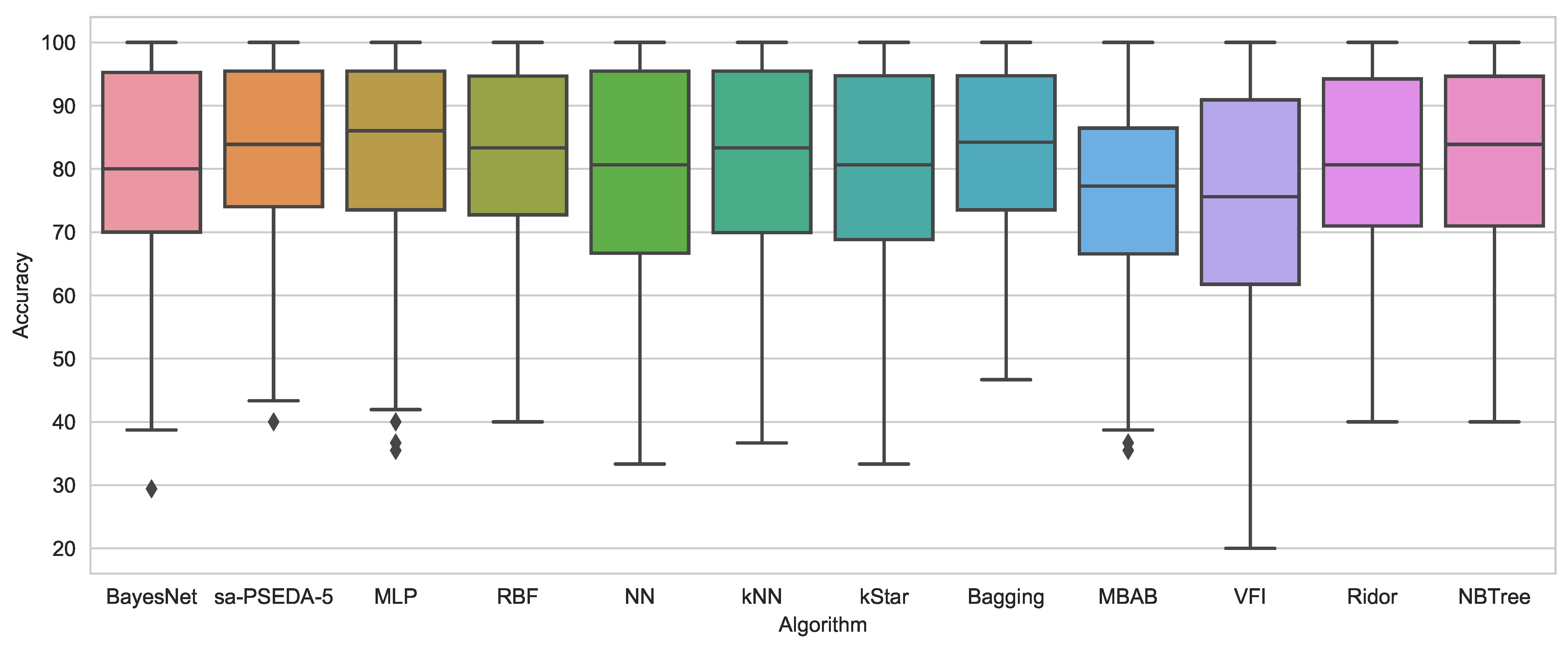
It is worth noticing, with reference to Figure 3, that MLP displays longer whiskers than sa–PSEDA-${\psi }_5$, which also has fewer non-classified (outliers) points and a more contained box (i.e., upper and lower quartile range). This highlights some instability for the MLP method. This is confirmed by the fact that, concerning the statistical analyses shown in Table 6, the proposed approach displays the best performance.

To further understand the potential of the proposed method for medical diagnosis and prognosis, the algorithms returning the best, second-best and third-best accuracy values are listed next to each corresponding classification problem in

Table 7. Best classification methods (sa–PSEDA-${\psi }_5$ plus 11 state-of-the-art algorithms).

Dataset	Most Performant	2nd Most Perf.	3rd Most Perf.
Breast-Real	sa–PSEDA-${\mathbf{\psi }}_{\mathbf{5}}$	kNN	MLP
Breast-Integer	BayesNet	kNN	sa–PSEDA-${\mathbf{\psi }}_{\mathbf{5}}$
Dermatology	BayesNet	MLP	kNN
Diabetes	sa–PSEDA-${\mathbf{\psi }}_{\mathbf{5}}$	Bagging	BayesNet
Haberman	sa–PSEDA-${\mathbf{\psi }}_{\mathbf{5}}$	MLP	RBF
Heart-2C	sa–PSEDA-${\mathbf{\psi }}_{\mathbf{5}}$	BayesNet	RBF
Heart-5C	BayesNet	sa–PSEDA-${\mathbf{\psi }}_{\mathbf{5}}$	RBF
Liver	Bagging	MLP	sa–PSEDA-${\mathbf{\psi }}_{\mathbf{5}}$
Parkinsons	NN	kNN	MLP
Thyroid	NN	sa–PSEDA-${\mathbf{\psi }}_{\mathbf{5}}$	MLP
Vertebral	MLP	Bagging	RBF
All	MLP	sa–PSEDA-${\mathbf{\psi }}_{\mathbf{5}}$	Bagging

.

Without considering the sa–PSEDA instances equipped with the other fitness functions, sa–PSEDA-${\psi }_5$ on its own appears in the table nine times and it is only missing in two datasets out of eleven.

7. Conclusions and Future Work

From the algorithmic point of view, the proposed sa-PSEDA algorithm appeared to be robust and more resilient to parameter variations than its predecessor PSEDA. This is interesting, as it comes to prove that the algorithmic design phase plays a major role in the metaheuristic optimisation field and that even a small variation in the algorithmic structure can lead to significantly better algorithmic structures. Moreover, this observation also shows that self-adaptation is key to good performances. This conclusion is coherent with the No Free Lunch Theorems in optimisation [68] and further confirms them.

As for the classification results, the proposed ODP method turned out to be extremely competitive against the chosen competitors, including the state-of-the-art classification algorithms from Weka, which are outperformed in several occasions. This is particularly evident when sa-PSEDA is used with the ${\psi }_5$ fitness function, which has proven to be the most adequate for the medical domain. This fitness function is not taken from the literature but is proposed in this article. Due to the obtained accuracy, we recommend its use while designing similar classification approaches.

Since a deterioration of the accuracy is noted in datasets containing a large number of outliers, future investigations will be carried out to deal with this issue. On top of designing a pre-processing phase to filter out outliers, we will focus on the algorithmic design to obtain a novel optimisation algorithm displaying a more robust structure. This should be doable by means of the EDA paradigm, as distributions can be updated so as to move their mean value away from outlier points. Alternatively, the use of multivariate Gaussian distribution could also help avoid this deterioration of the accuracy. Another future line of research is to handle the different types of search spaces (numerical, integer, binary) by means of the algebraic framework for evolutionary computations proposed in References [46,69,70].

References

- De Vos, B.D.; Berendsen, F.F.; Viergever, M.A.; Staring, M.; Išgum, I. End-to-End Unsupervised Deformable Image Registration with a Convolutional Neural Network. In Deep Learning in Medical Image Analysis and Multimodal Learning for Clinical Decision Support; Springer International Publishing: Cham, Switzerland, 2017; pp. 204–212. [Google Scholar] [CrossRef] [Green Version]
- Eppenhof, K.A.J.; Lafarge, M.W.; Moeskops, P.; Veta, M.; Pluim, J.P.W. Deformable image registration using convolutional neural networks. In Medical Imaging 2018: Image Processing; Angelini, E.D., Landman, B.A., Eds.; International Society for Optics and Photonics (SPIE): Houston, TX, USA, 2018; Volume 10574, pp. 192–197. [Google Scholar] [CrossRef]
- Erickson, B.J.; Korfiatis, P.; Akkus, Z.; Kline, T.L. Machine learning for medical imaging. Radiographics 2017, 37, 505–515. [Google Scholar] [CrossRef]
- Hu, J.; Chen, D.; Liang, P. A Novel Interval Three-Way Concept Lattice Model with Its Application in Medical Diagnosis. Mathematics 2019, 7, 103. [Google Scholar] [CrossRef]
- Hernaiz-Guijarro, M.; Castro-Palacio, J.C.; Navarro-Pardo, E.; Isidro, J.M.; Fernández-de Córdoba, P. A Probabilistic Classification Procedure Based on Response Time Analysis Towards a Quick Pre-Diagnosis of Student’s Attention Deficit. Mathematics 2019, 7, 473. [Google Scholar] [CrossRef]
- Maglogiannis, I.; Zafiropoulos, E.; Anagnostopoulos, I. An intelligent system for automated breast cancer diagnosis and prognosis using SVM based classifiers. Appl. Intell. 2009, 30, 24–36. [Google Scholar] [CrossRef]
- Kourou, K.; Exarchos, T.P.; Exarchos, K.P.; Karamouzis, M.V.; Fotiadis, D.I. Machine learning applications in cancer prognosis and prediction. Comput. Struct. Biotechnol. J. 2015, 13, 8–17. [Google Scholar] [CrossRef] [PubMed]
- Castaneda, C.; Nalley, K.; Mannion, C.; Bhattacharyya, P.; Blake, P.; Pecora, A.; Goy, A.; Suh, K.S. Clinical decision support systems for improving diagnostic accuracy and achieving precision medicine. J. Clin. Bioinform. 2015, 5, 4. [Google Scholar] [CrossRef] [Green Version]
- Abu-Nasser, B. Medical Expert Systems Survey. Int. J. Eng. Inf. Syst. 2017, 1, 218–224. [Google Scholar]
- Rajkomar, A.; Dean, J.; Kohane, I. Machine Learning in Medicine. N. Engl. J. Med. 2019, 380, 1347–1358. [Google Scholar] [CrossRef]
- Lin, W.; Tong, T.; Gao, Q.; Guo, D.; Du, X.; Yang, Y.; Guo, G.; Xiao, M.; Du, M.; Qu, X. Convolutional Neural Networks-Based MRI Image Analysis for the Alzheimer’s Disease Prediction From Mild Cognitive Impairment. Front. Neurosci. 2018, 12, 777. [Google Scholar] [CrossRef]
- Amezquita-Sanchez, J.P.; Mammone, N.; Morabito, F.C.; Marino, S.; Adeli, H. A novel methodology for automated differential diagnosis of mild cognitive impairment and the Alzheimer’s disease using EEG signals. J. Neurosci. Methods 2019, 322, 88–95. [Google Scholar] [CrossRef]
- Pereira, S.; Pinto, A.; Alves, V.; Silva, C.A. Brain Tumor Segmentation Using Convolutional Neural Networks in MRI Images. IEEE Trans. Med Imaging 2016, 35, 1240–1251. [Google Scholar] [CrossRef] [PubMed]
- Korolev, S.; Safiullin, A.; Belyaev, M.; Dodonova, Y. Residual and plain convolutional neural networks for 3D brain MRI classification. In Proceedings of the 2017 IEEE 14th International Symposium on Biomedical Imaging (ISBI 2017), Melbourne, Australia, 18–21 April 2017; pp. 835–838. [Google Scholar] [CrossRef]
- Hoseini, F.; Shahbahrami, A.; Bayat, P. An Efficient Implementation of Deep Convolutional Neural Networks for MRI Segmentation. J. Digit. Imaging 2018, 31, 738–747. [Google Scholar] [CrossRef] [PubMed]
- Collste, G. Expert systems in medicine and moral responsibility. J. Syst. Softw. 1992, 17, 15–22. [Google Scholar] [CrossRef]
- Shameer, K.; Johnson, K.W.; Glicksberg, B.S.; Dudley, J.T.; Sengupta, P.P. Machine learning in cardiovascular medicine: Are we there yet? Heart 2018, 104, 1156–1164. [Google Scholar] [CrossRef]
- Schrider, D.R.; Kern, A.D. Supervised Machine Learning for Population Genetics: A New Paradigm. Trends Genet. 2018, 34, 301–312. [Google Scholar] [CrossRef] [PubMed] [Green Version]
- Santucci, V.; Milani, A. Particle Swarm Optimization in the EDAs Framework. In Soft Computing in Industrial Applications; Springer: Berlin/Heidelberg, Germany, 2011; Volume 96, pp. 87–96. [Google Scholar]
- Kennedy, J.; Eberhart, R. Particle swarm optimization. In Proceedings of the IEEE International Conference on Neural Networks, Perth, Australia, 27 November–1 December 1995; Volume 4, pp. 1942–1948. [Google Scholar]
- Baioletti, M.; Milani, A.; Santucci, V. A New Precedence-Based Ant Colony Optimization for Permutation Problems. In Simulated Evolution and Learning; Springer International Publishing: Cham, Switzerland, 2017; pp. 960–971. [Google Scholar]
- Santucci, V.; Baioletti, M.; Milani, A. Tackling Permutation-based Optimization Problems with an Algebraic Particle Swarm Optimization Algorithm. Fundam. Inform. 2019, 167, 133–158. [Google Scholar] [CrossRef]
- Milani, A.; Santucci, V. Asynchronous differential evolution. In Proceedings of the IEEE Congress on Evolutionary Computation, Portland, OR, USA, 19–23 June 2004; pp. 1–7. [Google Scholar]
- Eiben, A.E.; Smith, J.E. Introduction to Evolutionary Computing; Springer: Berlin/Heidelberg, Germany, 2003; Volume 53. [Google Scholar]
- Kononova, A.V.; Corne, D.W.; Wilde, P.D.; Shneer, V.; Caraffini, F. Structural bias in population-based algorithms. Inf. Sci. 2015, 298, 468–490. [Google Scholar] [CrossRef] [Green Version]
- Zhang, Y.; Wang, S.; Ji, G. A comprehensive survey on particle swarm optimization algorithm and its applications. Math. Probl. Eng. 2015, 2015, 931256. [Google Scholar] [CrossRef]
- Kong, F.; Jiang, J.; Huang, Y. An Adaptive Multi-Swarm Competition Particle Swarm Optimizer for Large-Scale Optimization. Mathematics 2019, 7, 521. [Google Scholar] [CrossRef]
- Guo, W.; Zhu, L.; Wang, L.; Wu, Q.; Kong, F. An Entropy-Assisted Particle Swarm Optimizer for Large-Scale Optimization Problem. Mathematics 2019, 7, 414. [Google Scholar] [CrossRef]
- Elbes, M.; Alzubi, S.; Kanan, T.; Al-Fuqaha, A.; Hawashin, B. A survey on particle swarm optimization with emphasis on engineering and network applications. Evol. Intell. 2019, 12, 113–129. [Google Scholar] [CrossRef]
- Iacca, G.; Caraffini, F.; Neri, F. Milti-Strategy Coevolving Aging Particle Optimization. Int. J. Neural Syst. 2014, 24, 1450008. [Google Scholar] [CrossRef] [PubMed]
- El-Abd, M.; Kamel, M. PSO_Bounds: A New Hybridization Technique of PSO and EDAs. Found. Comput. Intell. 2009, 3, 509–526. [Google Scholar]
- Iacca, G.; Caraffini, F. Compact Optimization Algorithms with Re-Sampled Inheritance. In Applications of Evolutionary Computation; Kaufmann, P., Castillo, P.A., Eds.; Springer International Publishing: Cham, Switzerland, 2019; pp. 523–534. [Google Scholar] [CrossRef] [Green Version]
- Iacca, G.; Caraffini, F.; Neri, F. Compact Differential Evolution Light: High Performance Despite Limited Memory Requirement and Modest Computational Overhead. J. Comput. Sci. Technol. 2012, 27, 1056–1076. [Google Scholar] [CrossRef]
- Pelikan, M.; Goldberg, D.E.; Cantu-Paz, E. Linkage problem, distribution estimation, and Bayesian networks. Evol. Comput. 2000, 8, 311–340. [Google Scholar] [CrossRef]
- Kulkarni, R.; Venayagamoorthy, G. An estimation of distribution improved particle swarm optimization algorithm. In Proceedings of the ISSNIP 2007 3rd International Conference on Intelligent Sensors, Sensor Networks and Information, London, UK, 3–6 December 2007; pp. 539–544. [Google Scholar]
- Li, J.; Zhang, J.; Jiang, C.; Zhou, M. Composite particle swarm optimizer with historical memory for function optimization. IEEE Trans. Cybern. 2015, 45, 2350–2363. [Google Scholar] [CrossRef]
- Diker, A.; Avci, D.; Avci, E.; Gedikpinar, M. A new technique for ECG signal classification genetic algorithm Wavelet Kernel extreme learning machine. Optik 2019, 180, 46–55. [Google Scholar] [CrossRef]
- Ghosh, M.; Begum, S.; Sarkar, R.; Chakraborty, D.; Maulik, U. Recursive Memetic Algorithm for gene selection in microarray data. Expert Syst. Appl. 2019, 116, 172–185. [Google Scholar] [CrossRef]
- De Falco, I.; Della Cioppa, A.; Tarantino, E. Facing classification problems with particle swarm optimization. Appl. Soft Comput. 2007, 7, 652–658. [Google Scholar] [CrossRef]
- Karaboga, D.; Ozturk, C. A novel clustering approach: Artificial Bee Colony (ABC) algorithm. Appl. Soft Comput. 2011, 11, 652–657. [Google Scholar] [CrossRef]
- Frank, A.; Asuncion, A. UCI Machine Learning Repository; University of California, School of Information and Computer Science: Irvine, CA, USA, 2010. [Google Scholar]
- Hall, M.; Frank, E.; Holmes, G.; Pfahringer, B.; Reutemann, P.; Witten, I.H. The WEKA data mining software: An update. SIGKDD Explor. Newsl. 2009, 11, 10–18. [Google Scholar] [CrossRef]
- Caraffini, F.; Kononova, A.V. Structural bias in differential evolution: A preliminary study. In AIP Conference Proceedings; AIP Publishings: Leiden, The Netherlands, 2019; Volume 2070, p. 020005. [Google Scholar] [CrossRef]
- Caraffini, F.; Kononova, A.V.; Corne, D. Infeasibility and structural bias in differential evolution. Inf. Sci. 2019, 496, 161–179. [Google Scholar] [CrossRef] [Green Version]
- Titterington, D.; Smith, A.; Makov, U. Statistical Analysis of Finite Mixture Distributions; Wiley: New York, NY, USA, 1985; Volume 38. [Google Scholar]
- Baioletti, M.; Milani, A.; Santucci, V. MOEA/DEP: An algebraic decomposition-based evolutionary algorithm for the multiobjective permutation flowshop scheduling problem. In European Conference on Evolutionary Computation in Combinatorial Optimization; Springer: Cham, Switzerland, 2018; pp. 132–145. [Google Scholar]
- Choudhary, R.; Gianey, H.K. Comprehensive Review On Supervised Machine Learning Algorithms. In Proceedings of the 2017 International Conference on Machine Learning and Data Science (MLDS), Noida, India, 14–15 December 2017; pp. 37–43. [Google Scholar]
- Liu, Z.T.; Wu, M.; Cao, W.H.; Mao, J.W.; Xu, J.P.; Tan, G.Z. Speech emotion recognition based on feature selection and extreme learning machine decision tree. Neurocomputing 2018, 273, 271–280. [Google Scholar] [CrossRef]
- Moodley, R.; Chiclana, F.; Caraffini, F.; Carter, J. Application of uninorms to market basket analysis. Int. J. Intell. Syst. 2019, 34, 39–49. [Google Scholar] [CrossRef]
- Moodley, R.; Chiclana, F.; Caraffini, F.; Carter, J. A product-centric data mining algorithm for targeted promotions. J. Retail. Consum. Serv. 2019, 101940. [Google Scholar] [CrossRef]
- Mohammed, M.A.; Abd Ghani, M.K.; Arunkumar, N.; Hamed, R.I.; Mostafa, S.A.; Abdullah, M.K.; Burhanuddin, M.A. Decision support system for nasopharyngeal carcinoma discrimination from endoscopic images using artificial neural network. J. Supercomput. 2018. [Google Scholar] [CrossRef]
- Peña, A.; Bonet, I.; Manzur, D.; Góngora, M.; Caraffini, F. Validation of convolutional layers in deep learning models to identify patterns in multispectral images. In Proceedings of the 2019 14th Iberian Conference on Information Systems and Technologies (CISTI), Coimbra, Portugal, 19–22 June 2019; pp. 1–6. [Google Scholar] [CrossRef]
- Rocchio, J. Relevance Feedback in Information Retrieval. In SMART Retrieval System Experimens in Automatic Document Processing; Prentice-Hall, Inc.: Upper Saddle River, NJ, USA, 1971. [Google Scholar]
- Caraffini, F. The Stochastic Optimisation Software (SOS) Platform; Zenodo: Geneva, Switzerland, 2019. [Google Scholar]
- Levner, I. Feature selection and nearest centroid classification for protein mass spectrometry. BMC Bioinform. 2005, 6, 68. [Google Scholar] [CrossRef]
- Jensen, F. An Introduction to Bayesian Networks; UCL Press: London, UK, 1996; Volume 74. [Google Scholar]
- Rumelhart, D.; Hintont, G.; Williams, R. Learning representations by back-propagating errors. Nature 1986, 323, 533–536. [Google Scholar] [CrossRef]
- Hassoun, M. Fundamentals of Artificial Neural Networks; MIT Press: Cambridge, MA, USA, 1995. [Google Scholar]
- Cover, T.; Hart, P. Nearest neighbor pattern classification. IEEE Trans. Inf. Theory 1967, 13, 21–27. [Google Scholar] [CrossRef]
- Cleary, J.G.; Trigg, L.E. K*: An Instance-based Learner Using an Entropic Distance Measure. In Proceedings of the 12th International Conference on Machine Learning, Morgan Kaufmann, Nashville, TN, USA, 9–12 July 1995; pp. 108–114. [Google Scholar]
- Breiman, L. Bagging predictors. Mach. Learn. 1996, 24, 123–140. [Google Scholar] [CrossRef] [Green Version]
- Webb, G. Multiboosting: A technique for combining boosting and wagging. MAchine Learn. 2000, 40, 159–196. [Google Scholar] [CrossRef]
- Compton, P.; Jansen, R. Knowledge in context: A strategy for expert system maintenance. In Lecture Notes in Computer Science; Barter, C., Brooks, M., Eds.; AI ’88; Springer: Berlin/Heidelberg, Germany, 1990; Volume 406, pp. 292–306. [Google Scholar] [CrossRef]
- Kohavi, R. Scaling up the accuracy of naive-Bayes classifiers: A decision-tree hybrid. In Proceedings of the Second International Conference on Knowledge Discovery and Data Mining, Portland, OR, USA, 2–4 August 1996; Volume 7. [Google Scholar]
- Demiröz, G.; Güvenir, H. Classification by voting feature intervals. In Machine Learning: ECML-97; Springer: Berlin/Heidelberg, Germany, 1997; pp. 85–92. [Google Scholar]
- Tilahun, S.L.; Ngnotchouye, J.M.T.; Hamadneh, N.N. Continuous versions of firefly algorithm: A review. Artif. Intell. Rev. 2019, 51, 445–492. [Google Scholar] [CrossRef]
- Caraffini, F.; Neri, F. A study on rotation invariance in differential evolution. Swarm Evol. Comput. 2018, 100436. [Google Scholar] [CrossRef]
- Wolpert, D.H.; Macready, W.G. No free lunch theorems for optimization. IEEE Trans. Evol. Comput. 1997, 1, 67–82. [Google Scholar] [CrossRef] [Green Version]
- Baioletti, M.; Milani, A.; Santucci, V. Automatic Algebraic Evolutionary Algorithms. In International Workshop on Artificial Life and Evolutionary Computation (WIVACE 2017); Springer International Publishing: Cham, Switzerland, 2018; pp. 271–283. [Google Scholar] [CrossRef]
- Baioletti, M.; Milani, A.; Santucci, V. Learning Bayesian Networks with Algebraic Differential Evolution. In 15th International Conference on Parallel Problem Solving from Nature—PPSN XV; Springer International Publishing: Cham, Switzerland, 2018; pp. 436–448. [Google Scholar] [CrossRef]
Figure 1.
Box plots for sa-PSEDA equipped with the five fitness functions under study.
Figure 2.
Average fitness trends for the SI classifiers (equipped with ) and the NC classifier.
Figure 3.
Box plots for sa-PSEDA- and the 11 state-of-the-art classification schemes from Reference [42].