Significance of Double Stratification in Stagnation Point Flow of Third-Grade Fluid towards a Radiative Stretching Cylinder


Abstract
:1. Introduction
2. Formulation
3. Optimal Homotopic Solutions
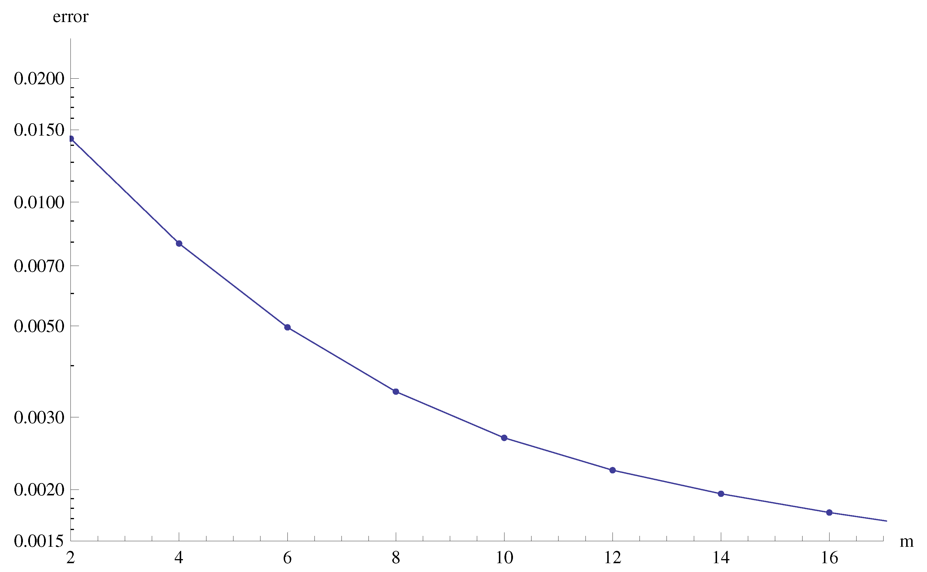
4. Optimal Convergence Control Parameters
5. Discussions
6. Concluding Remarks
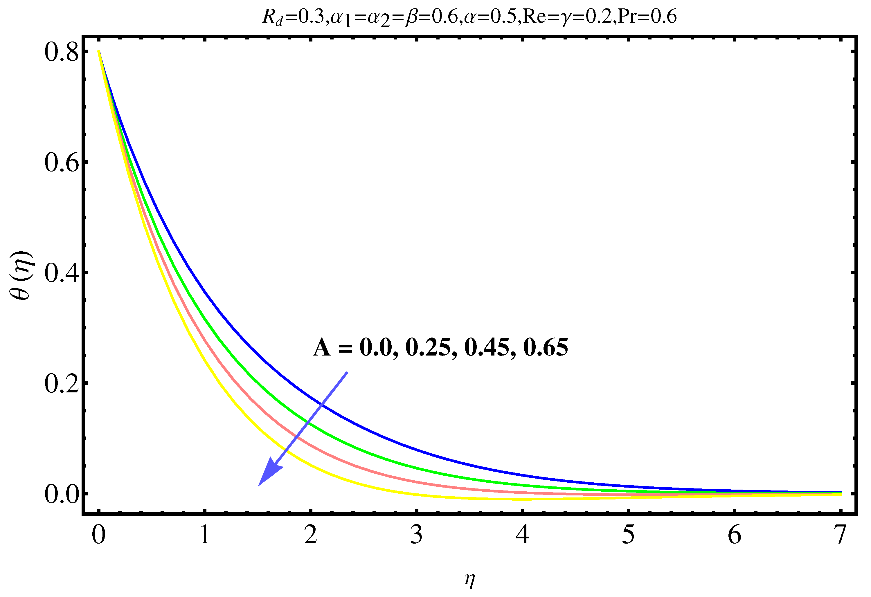
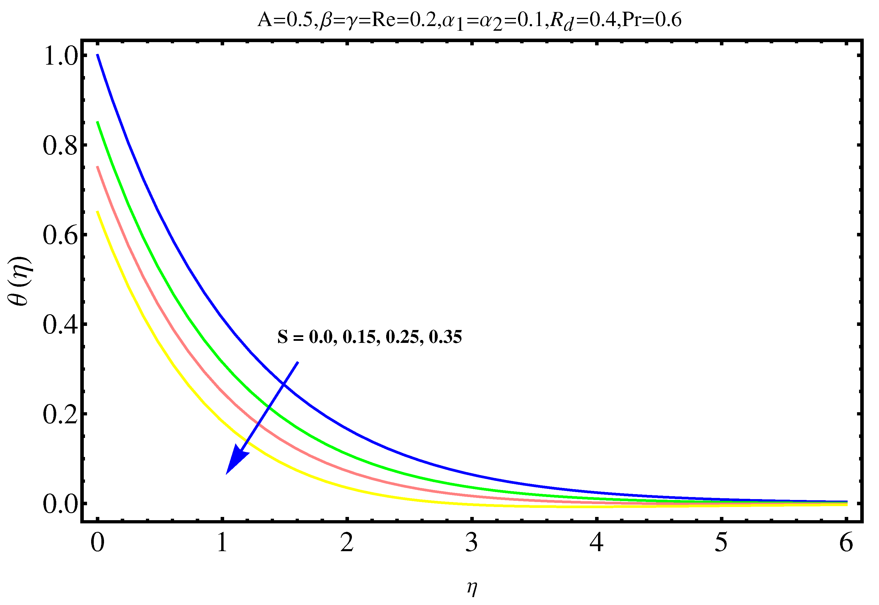
- Due to the effect of temperature, smaller values of stratified parameters results in higher values of velocity and temperature distributions.
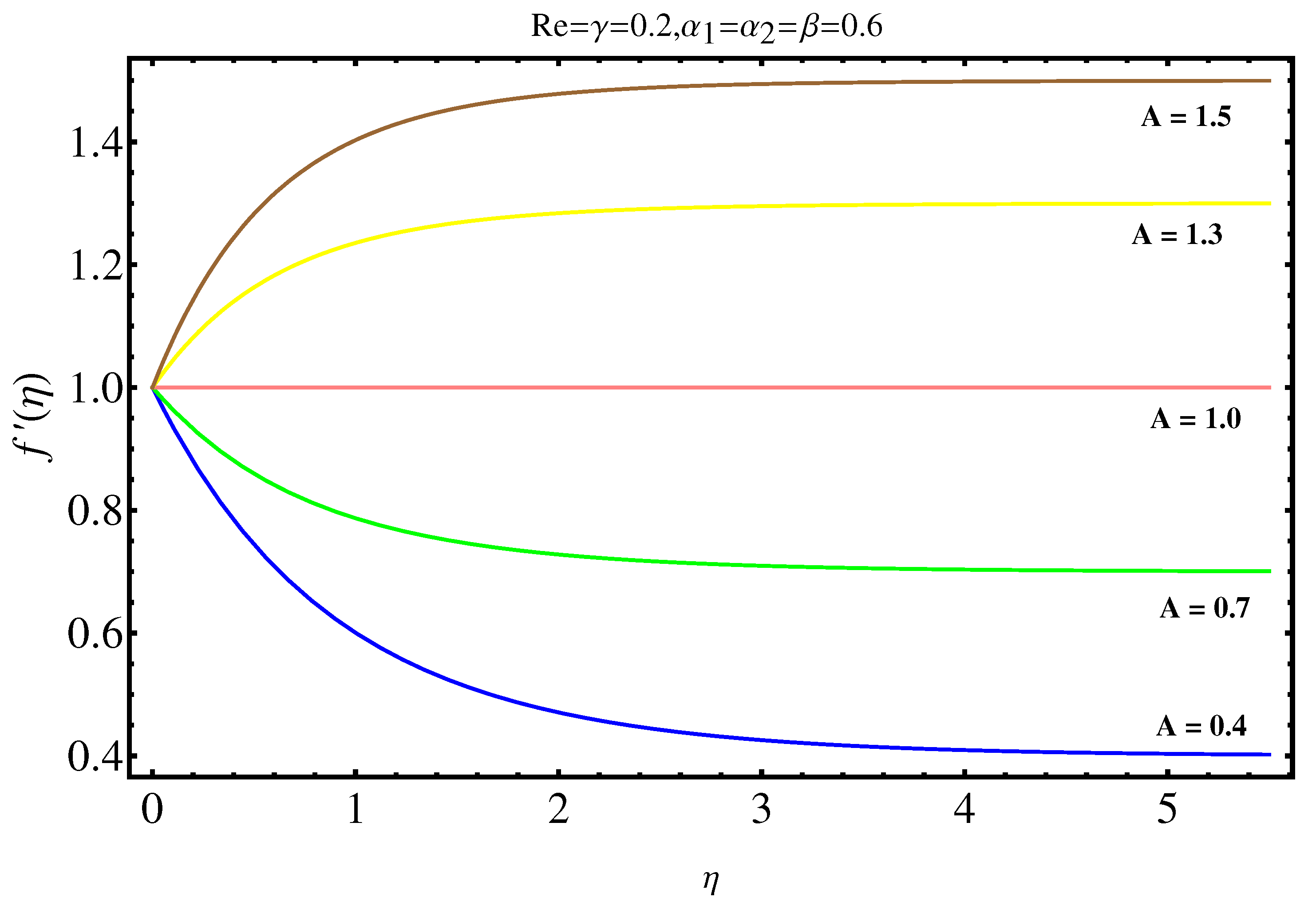
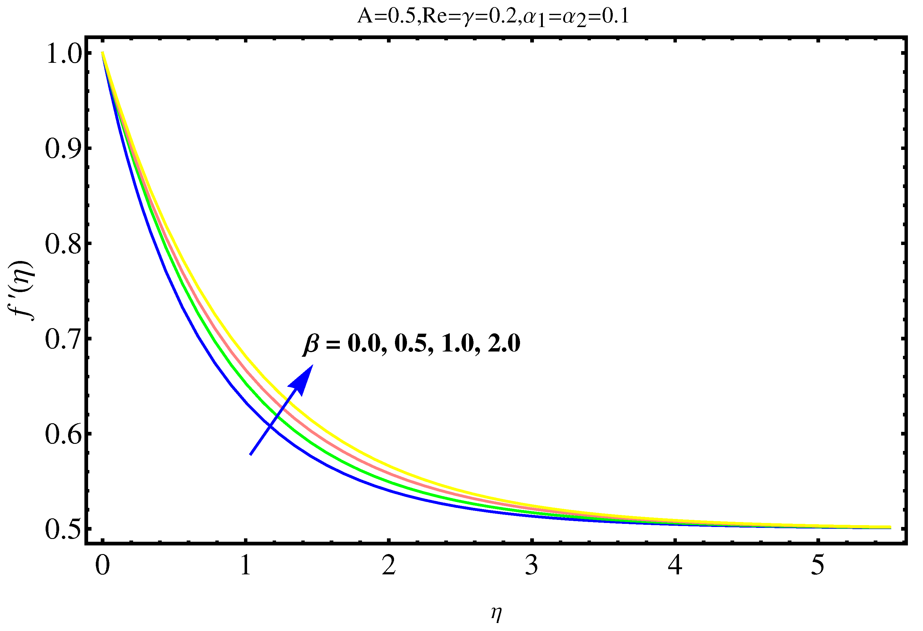
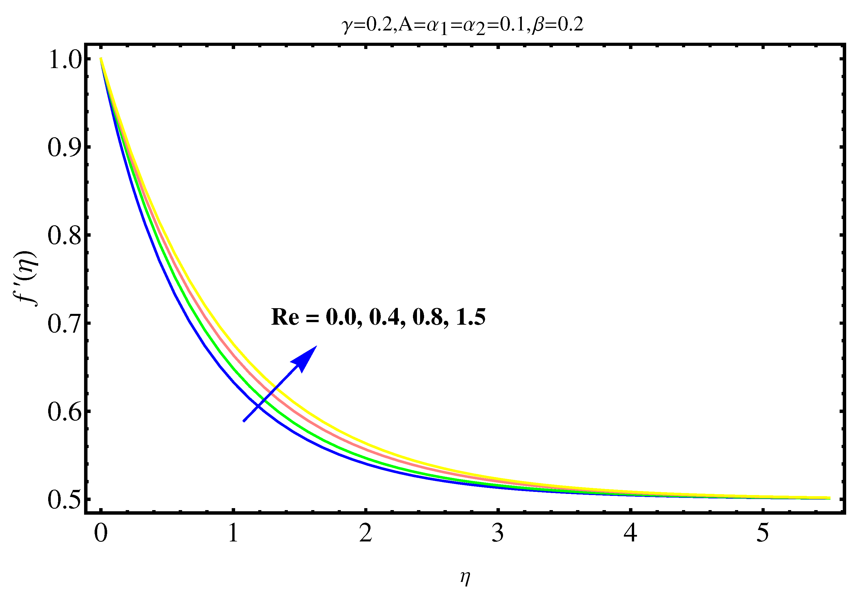
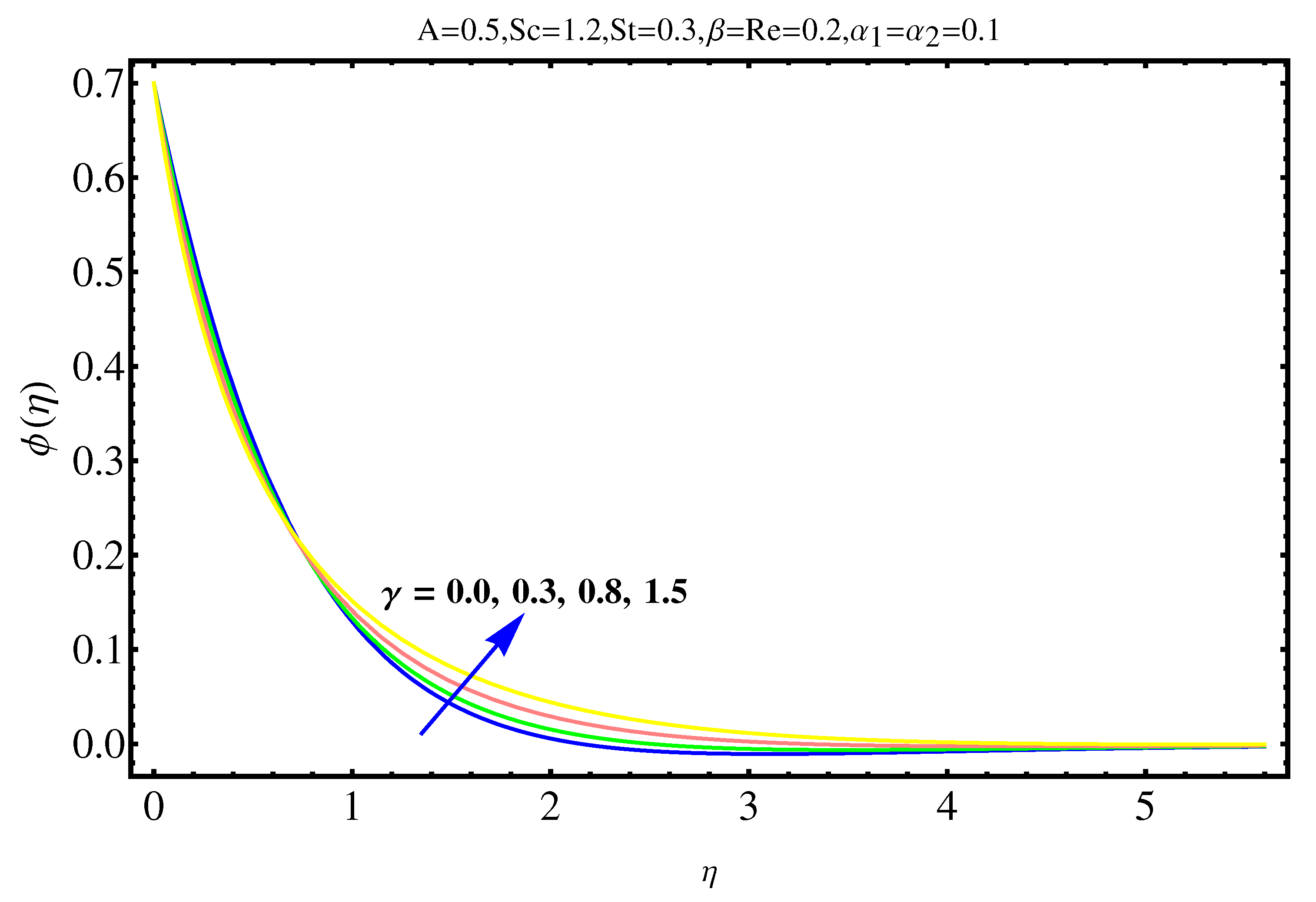
- Velocity profile enhances with and
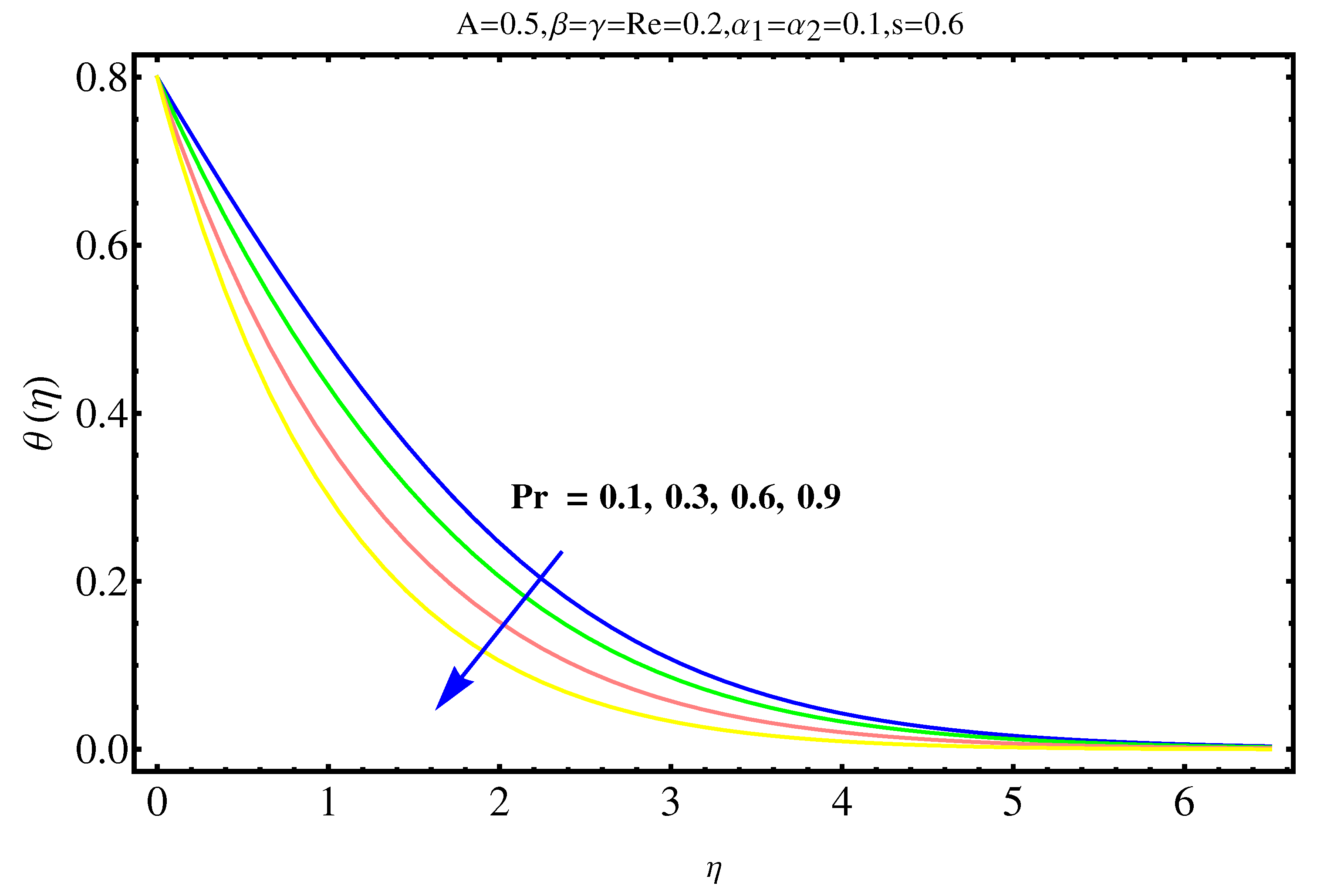
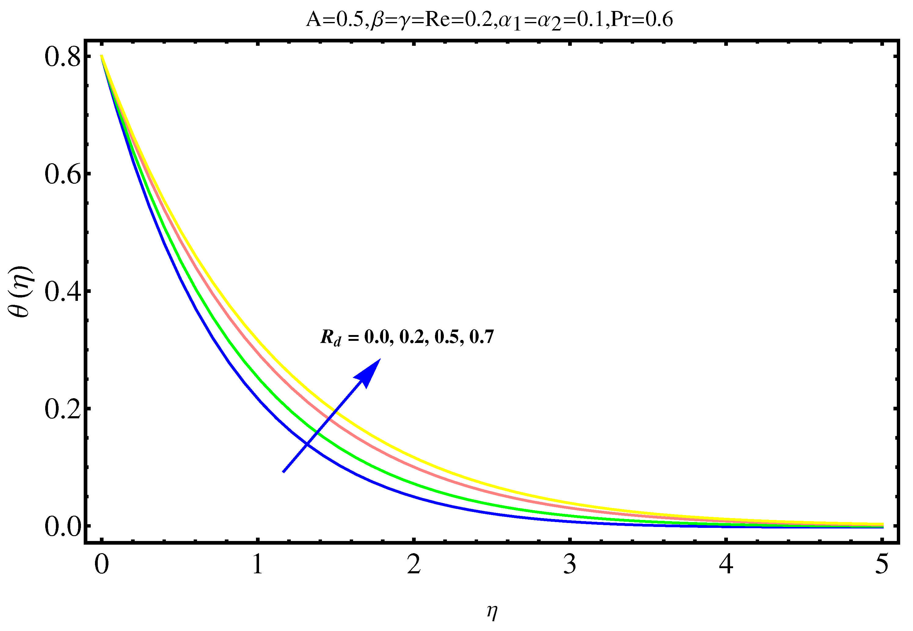
- Radiation parameter enhances while ratio parameter reduces the temperature distribution.
- The coefficient of skin friction is higher for higher values of and .
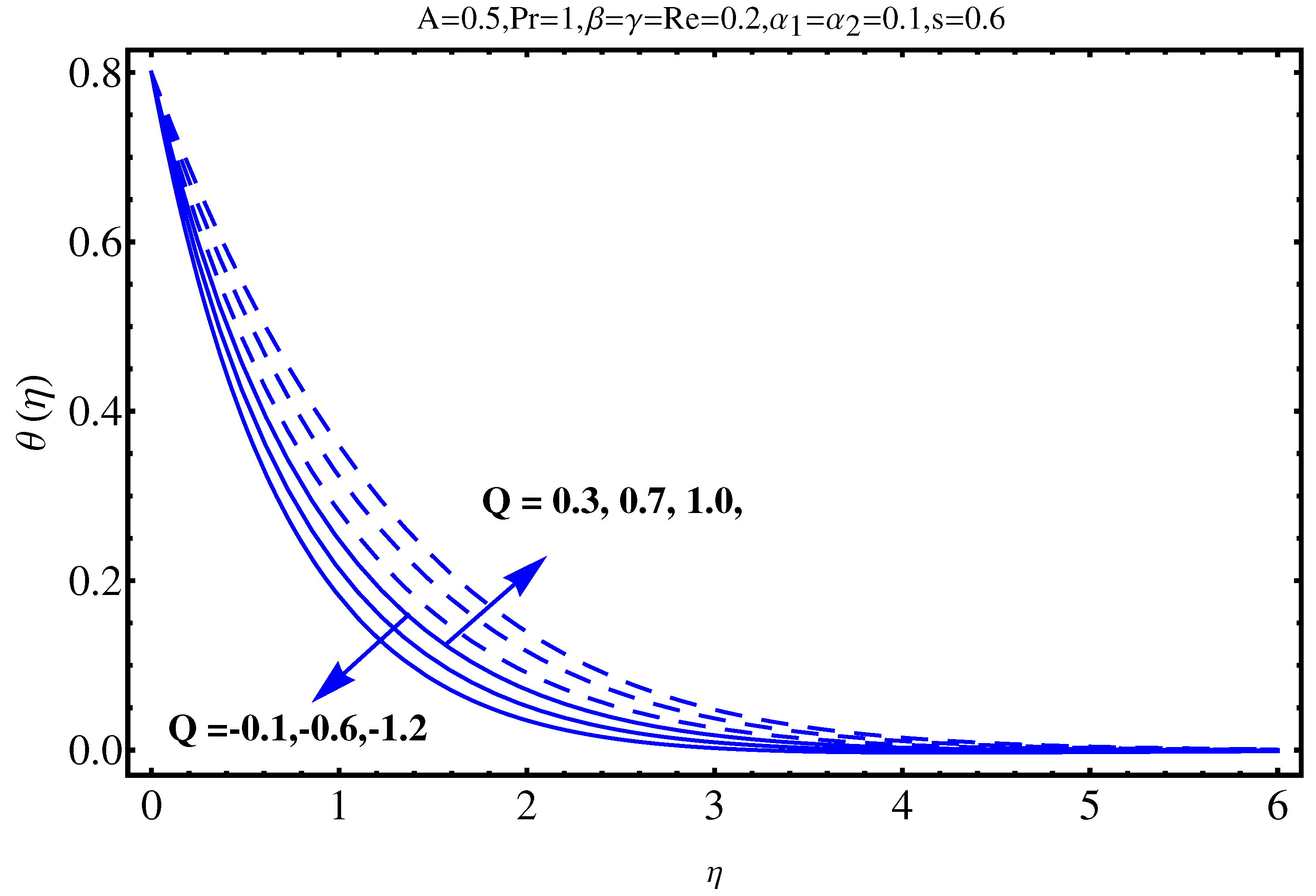
- An increase in Q and results in more convenient heat transfer.
Author Contributions
Funding
Conflicts of Interest
References
- Srinivasachariya, D.; RamReddy, C. Effect of double stratification on free convection in a micropolar fluid. ASME J. Heat Transf. 2011, 133, 1–7. [Google Scholar] [CrossRef]
- Srinivasachariya, D.; RamReddy, C. Free convective heat and mass transfer in a doubly stratified non-Darcy micro polar fluid. Korea J. Chem. Eng. 2011, 9, 1924–1932. [Google Scholar]
- Srinivasachariya, D.; RamReddy, C. Heat and mass transfer by natural convection in a doubly stratified non-Darcy micro polar fluid. Int. Commun. Heat Mass Transf. 2010, 37, 873–880. [Google Scholar] [CrossRef]
- Ibrahim, W.; Makinde, O.D. The effect of double stratification on boundary-layer flow and heat transfer of nanofluid over a vertical plate. Comput. Fluids 2013, 86, 433–441. [Google Scholar] [CrossRef]
- Shafiq, A.; Hammouch, Z.; Turab, A. Impact of Radiation in a Stagnation Point Flow of Walters’ B Fluid Towards a Riga Plate. Therm. Sci. Eng. Prog. 2018, 6, 27–33. [Google Scholar] [CrossRef]
- Tooke, R.M.; Blyth, M.G. A note on oblique stagnation-point flow. Phys. Fluids 2008, 20, 033101. [Google Scholar] [CrossRef]
- Hiemenz, K. Die Grenzschicht an einem in dengleichfiirmingen Flussigkeits stromeing etauchten geraden Kreiszy linder. Dinglers Polym. J. 1911, 326, 321–410. [Google Scholar]
- Khan, W.A.; Pop, I. Flow near the two-dimensional stagnation-point on an infinite permeable wall with a homogeneous–heterogeneous reaction. Commun. Nonlinear Sci. Numer. Simul. 2010, 15, 3435–3443. [Google Scholar] [CrossRef]
- Ja’fari, M.; Rahimi, A.B. Axisymmetric stagnation-point flow and heat transfer of a viscous fluid on a moving plate with time-dependent axial velocity and uniform transpiration. ScientiaIranica 2013, 20, 152–161. [Google Scholar] [CrossRef]
- Mabood, F.; Shafiq, A.; Hayat, T.; Abelman, S. Radiation effects on stagnation point flow with melting heat transfer and second order slip. Results Phys. 2017, 7, 31–42. [Google Scholar] [CrossRef]
- Hayat, T.; Shafiq, A.; Alsaedi, A. Characteristics of magnetic field and melting heat transfer in stagnation point flow of Tangent-hyperbolic liquid. J. Magn. Magn. Mater. 2016, 405, 97–106. [Google Scholar] [CrossRef]
- Ghoshdastidar, P.S. Heat Transfer; Oxford University Press: Oxford, UK, 2004. [Google Scholar]
- Cheng, P. Heat transfer in geothermal systems. Adv. Heat Transf. 1978, 14, 1–105. [Google Scholar]
- Cheng, P. Natural convection in a porous medium: External flow. In Proceedings of the NATO Advanced Study in Natural Convection, Izmir, Turkey, 16–27 July 1984. [Google Scholar]
- Rasool, G.; Zhang, T. Characteristics of chemical reaction and convective boundary conditions in Powell-Eyring nanofluid flow along a radiative Riga plate. Heliyon 2019, 5, e01479. [Google Scholar] [CrossRef] [PubMed]
- Vasu, B.; Reddy, R.; Murthy, P.V.S.N. Thermophoresis on boundary layer heat and mass transfer flow of Walters-B fluid past a radiate plate with heat sink/source. Heat Mass Transf. 2017, 53, 1553–1570. [Google Scholar] [CrossRef]
- Rasool, G.; Shafiq, A.; Khalique, C.M.; Zhang, T. Magnetohydrodynamic Darcy Forchheimer nanofluid flow over nonlinear stretching sheet. Phys. Scr. 2019, 94, 105221. [Google Scholar] [CrossRef]
- Rasool, G.; Zhang, T. Darcy-Forchheimer nanofluidic flow manifested with Cattaneo-Christov theory of heat and mass flux over non-linearly stretching surface. PLoS ONE 2019, 14, e0221302. [Google Scholar] [CrossRef]
- Kuznetsov, A.V.; Nield, D.A. Natural convective boundary-layer flow of a nanofluid past a vertical plate. Int. J. Therm. Sci. 2010, 49, 243–307. [Google Scholar] [CrossRef]
- Lesnic, D.; Ingham, D.B.; Pop, I. Free convection boundary layer flow along a vertical surface in a porous medium with Newtonian heating. Int. J. Heat Mass Transf. 1999, 42, 2621–2627. [Google Scholar] [CrossRef]
- Hayat, T.; Shafiq, A.; Mustafa, M.; Alsaedi, A. Boundary-Layer Flow of Walters’ B Fluid with Newtonian Heating. Z. Naturforschung A 2015, 70, 301–395. [Google Scholar] [CrossRef]
- Hayat, T.; Shafiq, A.; Alsaedi, A. Hydromagnetic boundary layer flow of Williamson fluid in the presence of thermal radiation and Ohmic dissipation. Alex. Eng. J. 2016, 55, 2229–2240. [Google Scholar] [CrossRef]
- Provotorov, V.V.; Provotorova, E.N. Optimal control of the linearized Navier-Stokes system in a netlike domain. Vestnik Sankt-Peterburgskogo Universiteta Prikladnaya Matematika Informatika Protsessy Upravleniya 2017, 13, 431–443. [Google Scholar]
- Artemov, M.A.; Baranovskii, E.S.; Zhabko, A.P.; Provotorov, V.V. On a 3D model of non-isothermal flows in a pipeline network. J. Phys. Conf. Ser. 2019, 1203, 012094. [Google Scholar] [CrossRef]
- Rasool, G.; Zhang, T.; Shafiq, A. Second grade nanofluidic flow past a convectively heated vertical Riga plate. Phys. Scr. 2019, 94, 125212. [Google Scholar] [CrossRef]
- Rasool, G.; Zhang, T.; Shafiq, A.; Durur, H. Influence of chemical reaction on Marangoni convective flow of nanoliquid in the presence of Lorentz forces and thermal radiation: A numerical investigation. J. Adv. Nanotech. 2019, 1, 32–49. [Google Scholar] [CrossRef]
- Rasool, G.; Zhang, T.; Shafiq, A. Marangoni effect in second grade forced convective flow of water based nanofluid. J. Adv. Nanotech. 2019, 1, 50–61. [Google Scholar] [CrossRef]
- Shafiq, A.; Nawaz, M.; Hayat, T.; Alsaedi, A. Magnetohydrodynamic axisymmetric flow of a third-grade fluid between two porous disks. Brazi. J. Chem. Eng. (USA) 2013, 3, 599–609. [Google Scholar] [CrossRef]
- Rasool, G.; Shafiq, A.; Tlili, I. Marangoni convective nano-fluid flow over an electromagnetic actuator in the presence of first order chemical reaction. Heat Transf.-Asian Res. 2019. [Google Scholar] [CrossRef]
- Rasool, G.; Shafiq, A.; Durur, H. Darcy-Forchheimer relation in Magnetohydrodynamic Jeffrey nanofluid flow over stretching surface, Discrete and Continuous Dynamical Systems-Series S. Am. Inst. Math. Sci. 2019. accepted. [Google Scholar]
- Rasool, G.; Shafiq, A.; Khalique, C.M. Marangoni forced convective Casson type nanofluid flow in the presence of Lorentz force generated by Riga plate, Discrete and Continuous Dynamical Systems - Series S. Am. Inst. Math. Sci. 2019. accepted. [Google Scholar]
Sample Availability: Samples of the compounds ...... are available from the authors. |


| m | Time [s] | |||
|---|---|---|---|---|
| 10 | ||||
| 14 | ||||
| 18 | ||||
| 20 |
| A | Re | |||||
|---|---|---|---|---|---|---|
| 0.0 | 0.1 | 0.1 | 0.2 | 0.6 | 0.4 | 1.04320 |
| 0.1 | 1.16269 | |||||
| 0.2 | 1.19544 | |||||
| 0.1 | 0.0 | 0.1 | 0.2 | 0.6 | 0.4 | 0.58384 |
| 0.1 | 0.57578 | |||||
| 0.2 | 0.56811 | |||||
| 0.1 | 0.1 | 0.0 | 0.2 | 0.6 | 0.4 | 0.57440 |
| 0.1 | 0.57718 | |||||
| 0.2 | 0.57985 | |||||
| 0.1 | 0.1 | 0.1 | 0.0 | 0.6 | 0.4 | 0.57310 |
| 0.1 | 0.57440 | |||||
| 0.2 | 0.57578 | |||||
| 0.1 | 0.1 | 0.1 | 0.2 | 0.0 | 0.4 | 1.21411 |
| 0.1 | 1.16269 | |||||
| 0.2 | 1.09544 | |||||
| 0.0 | 0.1 | 0.1 | 0.2 | 0.6 | 0.0 | 0.58381 |
| 0.1 | 0.64578 | |||||
| 0.2 | 0.76811 |
| Pr | Q | A | |||||||
|---|---|---|---|---|---|---|---|---|---|
| 0.4 | 1.0 | 0.3 | 0.3 | 0.2 | 0.1 | 0.1 | 0.6 | 0.1 | 1.01341 |
| 0.7 | 1.36421 | ||||||||
| 1.0 | 1.65732 | ||||||||
| 0.3 | 0.1 | 0.3 | 0.3 | 0.2 | 0.1 | 0.1 | 0.6 | 0.1 | 1.41321 |
| 0.5 | 1.36969 | ||||||||
| 1.0 | 1.12294 | ||||||||
| 0.3 | 1.0 | 0.0 | 0.3 | 0.2 | 0.1 | 0.1 | 0.6 | 0.1 | 1.11411 |
| 0.5 | 1.26969 | ||||||||
| 1.0 | 1.39294 | ||||||||
| 0.3 | 1.0 | 0.3 | 0.0 | 0.2 | 0.1 | 0.1 | 0.6 | 0.1 | 1.38941 |
| 0.5 | 1.62315 | ||||||||
| 1.0 | 1.89561 | ||||||||
| 0.3 | 1.0 | 0.3 | 0.3 | 0.0 | 0.1 | 0.1 | 0.6 | 0.1 | 1.12303 |
| 0.1 | 1.35344 | ||||||||
| 0.5 | 1.67423 | ||||||||
| 0.0 | 1.0 | 0.3 | 0.3 | 0.2 | 0.0 | 0.1 | 0.6 | 0.1 | 1.12141 |
| 0.5 | 1.24922 | ||||||||
| 1.0 | 1.41034 | ||||||||
| 0.3 | 1.0 | 0.3 | 0.3 | 0.2 | 0.1 | 0.0 | 0.6 | 0.1 | 1.30312 |
| 0.5 | 1.32601 | ||||||||
| 1.0 | 1.38923 | ||||||||
| 0.3 | 1.0 | 0.3 | 0.3 | 0.2 | 0.1 | 1.0 | 0.0 | 0.1 | 1.12423 |
| 0.5 | 1.24921 | ||||||||
| 1.0 | 1.41235 | ||||||||
| 0.3 | 1.0 | 0.3 | 0.3 | 0.2 | 0.1 | 1.0 | 0.6 | 0.0 | 1.25309 |
| 0.5 | 1.31985 | ||||||||
| 1.0 | 1.51225 |
| S | |||||||
|---|---|---|---|---|---|---|---|
| 0.0 | 0.3 | 0.2 | 1.2 | 0.1 | 0.1 | 0.1 | 0.98740 |
| 0.1 | 0.92745 | ||||||
| 0.2 | 0.90462 | ||||||
| 0.3 | 0.0 | 0.2 | 1.2 | 0.1 | 0.1 | 0.1 | 1.98741 |
| 0.1 | 1.74501 | ||||||
| 0.2 | 1.25019 | ||||||
| 0.3 | 0.3 | 0.0 | 1.2 | 0.1 | 0.1 | 0.1 | 1.11523 |
| 0.1 | 1.32751 | ||||||
| 0.2 | 1.89154 | ||||||
| 0.3 | 0.3 | 0.2 | 0.0 | 0.1 | 0.1 | 0.1 | 0.54315 |
| 0.1 | 0.38612 | ||||||
| 0.2 | 0.18612 | ||||||
| 0.3 | 0.3 | 0.2 | 1.2 | 0.0 | 0.1 | 0.1 | 0.81913 |
| 0.1 | 0.83997 | ||||||
| 0.2 | 0.91251 | ||||||
| 0.3 | 0.3 | 0.2 | 1.2 | 0.1 | 0.0 | 0.1 | 1.28712 |
| 0.1 | 1.59874 | ||||||
| 0.2 | 1.98717 | ||||||
| 0.3 | 0.3 | 0.2 | 1.2 | 0.1 | 0.1 | 0.0 | 1.71231 |
| 0.1 | 1.82127 | ||||||
| 0.2 | 1.92351 |
© 2019 by the authors. Licensee MDPI, Basel, Switzerland. This article is an open access article distributed under the terms and conditions of the Creative Commons Attribution (CC BY) license (http://creativecommons.org/licenses/by/4.0/).
Share and Cite
Shafiq, A.; Khan, I.; Rasool, G.; Seikh, A.H.; Sherif, E.-S.M. Significance of Double Stratification in Stagnation Point Flow of Third-Grade Fluid towards a Radiative Stretching Cylinder. Mathematics 2019, 7, 1103. https://0-doi-org.brum.beds.ac.uk/10.3390/math7111103
Shafiq A, Khan I, Rasool G, Seikh AH, Sherif E-SM. Significance of Double Stratification in Stagnation Point Flow of Third-Grade Fluid towards a Radiative Stretching Cylinder. Mathematics. 2019; 7(11):1103. https://0-doi-org.brum.beds.ac.uk/10.3390/math7111103
Chicago/Turabian StyleShafiq, Anum, Ilyas Khan, Ghulam Rasool, Asiful H. Seikh, and El-Sayed M. Sherif. 2019. "Significance of Double Stratification in Stagnation Point Flow of Third-Grade Fluid towards a Radiative Stretching Cylinder" Mathematics 7, no. 11: 1103. https://0-doi-org.brum.beds.ac.uk/10.3390/math7111103