A New Criterion for Model Selection

Abstract

Selecting the best model from a set of candidates for a given set of data is obviously not an easy task. In this paper, we propose a new criterion that takes into account a larger penalty when adding too many coefficients (or estimated parameters) in the model from too small a sample in the presence of too much noise, in addition to minimizing the sum of squares error. We discuss several real applications that illustrate the proposed criterion and compare its results to some existing criteria based on a simulated data set and some real datasets including advertising budget data, newly collected heart blood pressure health data sets and software failure data.

1. Introduction

Model selection has become an important focus in recent years in statistical learning, machine learning, and big data analytics [1,2,3,4]. Currently there are several criteria in the literature for model selection. Many researchers [3,5,6,7,8,9,10,11] have studied the problem of selecting variables in regression in thepast three decades. Today it receives much attention due to growing areas in machine learning, data mining and data science. The mean squared error (MSE), root mean squared error (RMSE), R², Adjusted R², Akaike’s Information Criterion (AIC), Bayesian Information Criterion (BIC), AICc are among common criteria that have been used to measure model performance and select the best model from a set of potential models. Yet choosing an appropriate criterion on the basis of which to compare the many candidate models remains not an easy task to many analysts since some criteria may taking toll on the model size of estimated parameters while the others could emphasis more on the sample size of a given data.

In this paper, we discuss a new criterion PIC that can be used to select the best model among a set of candidate models. The proposed PIC takes into account a larger penalty from adding too many coefficients in the model when there is too small a sample. We also discuss briefly several common existing criteria include AIC, BIC, AICc, R², adjusted R², MSE, and RMSE. To illustrate the proposed criterion, we discuss the results based on a simulated data and some real applications including advertising budget data and recent collected heart blood pressure health data sets. The new PIC takes into account a larger penalty when there are too many coefficients to be estimated from too small a sample in the presence of too much noise.

2. Some Criteria for Model Comparisons

Suppose there are n observations on a response variable Y that relates to a set of independent variables: X₁, X₂, …, X_k−1 in the form of

$$Y=f\left(X_1,X_2,\dots ,X_{k-1}\right).$$

(1)

The statistical significance of model comparisons can be determined based on existing goodness-of-fit criteria in the literature [12]. In this section, we first briefly discuss some existing criteria that commonly used in model selection. Then we discuss a new PIC for selecting the best model from a set of candidates. Following are some common criteria, for instance.

The MSE measures the average of the squares deviation between the fitted values with the actual data observation [13]. The RMSE is the square root of the variance of the residuals or the square root of MSE. The coefficient of determinations R² or R² value measures the amount of variation accounted for the fitted model. It is frequently used to compare models and assess which model provides the best fit to the data. R² always increases with the model size. The adjusted R² is a modification to the R² which takes into account the number of estimated parameters or the number of explanatory variables in a model relative to the number of data points [14]. The adjusted R² gives the percentage of variation explained by only those independent variables that actually affect the dependent variable.

The AIC was introduced by Akaike [5] and is calculated by obtaining the maximum value of the likelihood function for the model and the penalty term due to the number of estimated parameters in the model. This criterion implies that by adding more parameters in the model, it improves the goodness of the fit but also increases the penalty imposed by adding more parameters.

The BIC was introduced by Schwarz [10]. The difference between these two criteria, BIC and AIC, isa penalty term. In BIC, it depends on the sample size n that shows how strongly they impacts the penalty of the number of parameters in the model while in AIC it does not depend on the sample size. When the sample size is small, there is likely that AIC will select models that include many parameters. The second order information criterion, called AICc, takes into account sample size by increasing the relative penalty for model complexity with small data sets. As n gets larger, AICc converges to AIC.

It should be noted that the lower value of MSE, RMSE, AIC, BIC, AICc indicates the better the model goodness-of-fit. Conversely, the larger the value of R², adjusted R² indicates better fit.

New PIC

We now discuss a new criterion for selecting a model among several candidate models. Suppose there are n observations on a response variable Y and (k − 1) explanatory variables X₁, X₂, …, X_k−1. Let

y_i be the ith response (dependent variable), i = 1, 2, …, n

ŷ_i be the fitted value of y_i

e_i be the ith residual, i.e., e_i = y_i − ŷ_i

From Equation (1), the sum of squared error can be defined as follows:

$$SSE={\displaystyle \sum _{i=1}^n{e}_i^2}={\displaystyle \sum _{i=1}^n{\left(y_i-{\widehat{y}}_i\right)}^2}$$

(2)

In general, the adjusted R² attaches a small penalty for adding more variables in the model. The difference between the adjusted R² and R² is usually slightly small unless there are too many unknown coefficients in the model to be estimated from too small a sample in the presence of too much noise. In other words, the adjusted R² penalizes the loss of degrees of freedom that result from adding independent variables to the model. Our motivation of this study is to propose a new criterion by addressing the above situation. According to the unbiased estimators of the adjusted R² and R² that, respectively, correct for the sample size and numbers of estimated coefficients, we can easily show that the following function $k\left(\frac{1-R_{adj}^2}{1-R^2}\right)$ or equivalently, that $k\left(\frac{n-1}{n-k}\right)$ indicates a larger penalty for adding too many coefficients (or estimated parameters) in the model from too small a sample in the presence of too much noise where n is the sample size and k is the number of estimated parameters.

Based on the above, we propose a new criterion, PIC, for selecting the best model. The PIC value of the model is as follows:

$$\mathrm{PIC}=\mathrm{SSE}+k\left(\frac{n-1}{n-k}\right)$$

(3)

where n is the number of observations in the model

  k is the number of estimated parameters or (k−1) explanatory variables in the model, and

  SSE is the sum of squares error as given in Equation (2).

Table 1. Some criteria model selection.

No.	Criteria	Formula
1	MSE	$\mathrm{MSE}=\frac{{\displaystyle \sum _{i=1}^n{\left(y_i-{\widehat{y}}_i\right)}^2}}{n-k}$	Measures the deviation between the fitted values with the actual data observation.
2	RMSE	$\mathrm{RMSE}=\sqrt{\frac{{\displaystyle \sum _{i=1}^n{\left(y_i-{\widehat{y}}_i\right)}^2}}{n-k}}$	The square root of the MSE.
3	R2	$R^2=1-\frac{{\displaystyle \sum _{i=1}^n{\left(y_i-{\widehat{y}}_i\right)}^2}}{{\displaystyle \sum _{i=1}^n{\left(y_i-\overline{y}\right)}^2}}$	Measures the amount of variation accounted for the fitted model.
4	Adj R2	$R_{adj}^2=1-\left(\frac{n-1}{n-k}\right)\left(1-R^2\right)$	Take into account a small penalty for adding more variables in the model.
5	AIC	$AIC=-2\log (L)+2k$	The model improves the goodness of the fit but also increases the penalty by adding more parameters.
6	BIC	$BIC=-2\log (L)+k\log (n)$	Depend on the sample size n that shows how strongly BIC impacts the penalty of the number of parameters in the model.
7	AICc	$AI{C}_c=-2\log (L)+2k+\frac{2k\left(k+1\right)}{n-k-1}$	AICc takes into account sample size by increasing the relative penalty for model complexity with small data sets.
8	PIC	$\begin{array}{l}\mathrm{PIC}=SSE+k\left(\frac{n-1}{n-k}\right)\\ \mathrm{where}SSE={\displaystyle \sum _{i=1}^n{\left(y_i-{\widehat{y}}_i\right)}^2}\end{array}$	This new criterion takes into account a larger the penalty when adding too many coefficients in the model when there is too small a sample.

presents a summary of criteria for model selection in this study. The best model from among candidate models is the one that yields the smaller the value of MSE, RMSE, AIC, BIC, AICc and the new criterion value given in Equation (3) or the larger the value of R², adjusted R².

3. Experimental Validation

3.1. Numerical Examples

In this section, we illustrate the proposed criterion based on a simulated data from a multiple linear regression with three independent variables X₁, X₂ and X₃ for a set of 100 observations (Case 1) and 20 observations (Case 2).

Case 1: 100 observations based on simulated data.

Table 2. A simulated dataset of 100 observations from a multiple linear regression consisting of 3 independent variables.

X1	X2	X3	Y
11	68.028164	0	21.46126
12	69.086446	0	23.28792
13	84.806730	1	18.71906
14	19.011313	1	18.50209
15	63.046323	1	22.37717
16	82.686964	1	24.19955
17	59.263664	1	20.64198
18	88.756598	0	29.50144
19	77.884304	1	24.49684
20	9.346073	0	27.15191

presents a list of the first 10 observations from the simulated data consisting of 100 observations based on a multiple linear regression function. From

Table 3. Criteria values of independent variables based on 100 simulated data observations consisting of three independent variables X₁, X₂, and X₃.

Criteria	X1, X2, X3	X1, X2	X1, X3	X2, X3	X1	X2	X3
MSE	2.715904	8.844676	3.632836	214.9156	9.259849	213.7444	217.8576
AIC	389.594	506.7012	417.7079	417.7079	510.3048	824.2031	826.1659
AICc	390.0151	506.9512	417.9579	417.9579	510.4285	824.3268	826.2896
BIC	400.0147	514.5167	425.5234	425.5234	515.5151	829.4134	831.3762
RMSE	1.648	2.974	1.906	14.66	3.043	14.62	14.76
R2	0.9879	0.9601	0.9836	0.02904	0.9578	0.0251	0.005776
Adjusted R2	0.9875	0.9592	0.9833	0.00902	0.9573	0.01515	−0.00437
PIC	264.8518	860.9954	355.4469	20849.88	909.4856	20948.97	21352.07

we can observe that based on the new proposed criterion the multiple regression models including all three independent variables provides the best fit. The results are also consistent with all of the criteria such as MSE, AIC, AICc, BIC, RMSE, R², and adjusted R².

Case 2: 20 observations.

Table 4. A simulated dataset of 20 observations from a multiple linear regression consisting of 3 independent variables.

X1	X2	X3	Y
11	68.028164	0	28.05442
12	69.086446	0	25.44146
13	84.806730	1	18.73395
14	19.011313	1	18.00611
15	63.046323	1	24.69284
16	82.686964	0	28.57457
17	59.263664	1	22.69636
18	88.756598	0	29.59276
19	77.884304	0	29.19881
20	9.346073	1	21.72717
21	80.920814	1	25.78641
22	91.528869	1	26.44676
23	13.096270	1	23.20765
24	5.530196	0	25.37850
25	73.659765	0	32.86512
26	47.619990	0	29.91239
27	84.961929	0	35.45651
28	67.516106	0	34.46896
29	16.024371	0	31.97531
30	9.566489	0	33.54677

presents a simulated data set consisting of 20 observations based on a multiple linear regression function. From

Table 5. Criteria values of independent variables based on 20 simulated data observations consisting of three independent variables X₁, X₂, and X₃.

Criteria	X1, X2, X3	X1, X2	X1, X3	X2, X3	X1	X2	X3
MSE	2.62764	8.934121	5.692996	9.909904	14.32623	23.55161	10.44582
AIC	81.6276	105.3009	96.2897	107.3718	113.8972	123.8301	107.5755
AICc	84.29427	106.8009	97.7897	108.8718	114.6031	124.536	108.2814
BIC	85.61053	108.2881	99.2769	110.359	115.8887	125.8216	109.567
RMSE	1.621	2.989	2.386	3.148	3.785	4.853	3.232
R2	0.9111	0.6792	0.7956	0.6442	0.4551	0.1046	0.6028
Adjusted R2	0.8945	0.6415	0.7715	0.6024	0.4248	0.05487	0.5807
PIC	46.79226	155.233	100.1339	171.8213	259.9833	426.0401	190.1359

we can observe that a multiple regression model including all three independent variables based on the new criterion provides the best fit from among all 7 models (see Table 5). This result is also consistent with all the criteria such as MSE, AIC, AICc, BIC, RMSE, R² and adjusted R².

3.2. Applications

In this section we demonstrate the proposed criterion with several real applications including advertising products, heart blood pressure health and software reliability analysis. Based on our preliminary study on the collected data, the multiple linear regression model assumption is appropriate to be used in our applications 1 and 2 to illustrate the model selection.

Application 1: Advertising Budget.

In this study, we use the advertising budget data set [15] to illustrate the proposed criterion where the sales for a particular product is a dependent variable of multiple regressionand the three different media channels such as TV, Radio, and News paper are independent variables. The advertising dataset consists of the sales of a product in 200 different markets (200 rows), together with advertising budgets for the product in each of those markets for three different media channels: TV, radio and newspaper. The sales are in thousands of units and the budget is in thousands of dollars.

Table 6. Advertising budget data in 200 different markets.

TV	Radio	Newspaper	Sales
230.1	37.8	69.2	22.1
44.5	39.3	45.1	10.4
17.2	45.9	69.3	9.3
151.5	41.3	58.5	18.5
180.8	10.8	58.4	12.9
8.7	48.9	75	7.2
57.5	32.8	23.5	11.8
120.2	19.6	11.6	13.2
8.6	2.1	1	4.8

shows the first few rows of the advertising budget data set.

We now discuss the results of the linear regression model using this advertising data. Figure 1 and Figure 2 present the data plot and the correction coefficients between the pairs of variables of the advertising budget data, respectively. It shows that the pair of Sales and TV variables has the highest correlation. This implies that the TV advertising has a direct positive effect on the Sale. Results also show that there is a statistical significant positive effect of both TV and Radio advertisings on the Sales. From

Table 7. The relative important metrics of all three media channels (TV, Radio, Newspaper).

	Relative importance metrics:
	Lmg	Last	First	Pratt
TV	0.65232505	0.6918832537	0.6143151	0.656553238
Radio	0.32187149	0.3080966738	0.3333566	0.344548723
Newspaper	0.02580346	0.0000200725	0.0523283	−0.001101961

, TV media is the most significant media among the three advertising channels and it has strongest impacts on the Sales. The R² is 0.8972, so 89.72% of the variability is explained by all three media channels. From

Table 8. Criteria values of independent variables (TV, Radio, Newspaper) of regression models. (X₁, X₂, and X₃ be denoted as the TV, Radio and Newspaper, respectively).

Criteria	X1, X2, X3	X1, X2	X1, X3	X2, X3	X1	X2	X3
MSE	2.8409	2.8270	9.7389	18.349	10.619	18.275	25.933
AIC	782.36	780.39	1027.8	1154.5	1044.1	1152.7	1222.7
AICc	782.49	780.46	1027.84	1154.53	1044.15	1152.74	1222.73
BIC	795.55	790.29	1037.7	1164.4	1050.7	1159.3	1229.3
RMSE	1.6855	1.6814	3.1207	4.2836	3.2587	4.2750	5.0925
R2	0.8972	0.8972	0.6458	0.3327	0.6119	0.3320	0.0521
Adjusted R2	0.8956	0.8962	0.6422	0.3259	0.6099	0.3287	0.0473
PIC	5.7467	4.7118	6.1512	7.3141	5.2688	6.2850	7.1026

, the values of R² with all three variables and just two variables (TV and Radio advertisings) in the model are the same. This implies that we can select the model with two variables (TV and Radio) in the regression. We can now examine the adjusted R² measure. For the regression model with TV and Radio variables, the adjust R² is 0.8962 while adding the third variable (Newspaper) into the model, the adjusted R² of the full model size is then reduced to 0.8956. Based on the new proposed criterion, the model with the two advertising media channels (TV and Radio) is the best model from a set of seven candidate models as shown in Table 8. This result is consistent with all criteria such as MSE, AIC, AICc, BIC, RMSE, and adjusted R².

Application 2: Heart Blood Pressure Health Data.

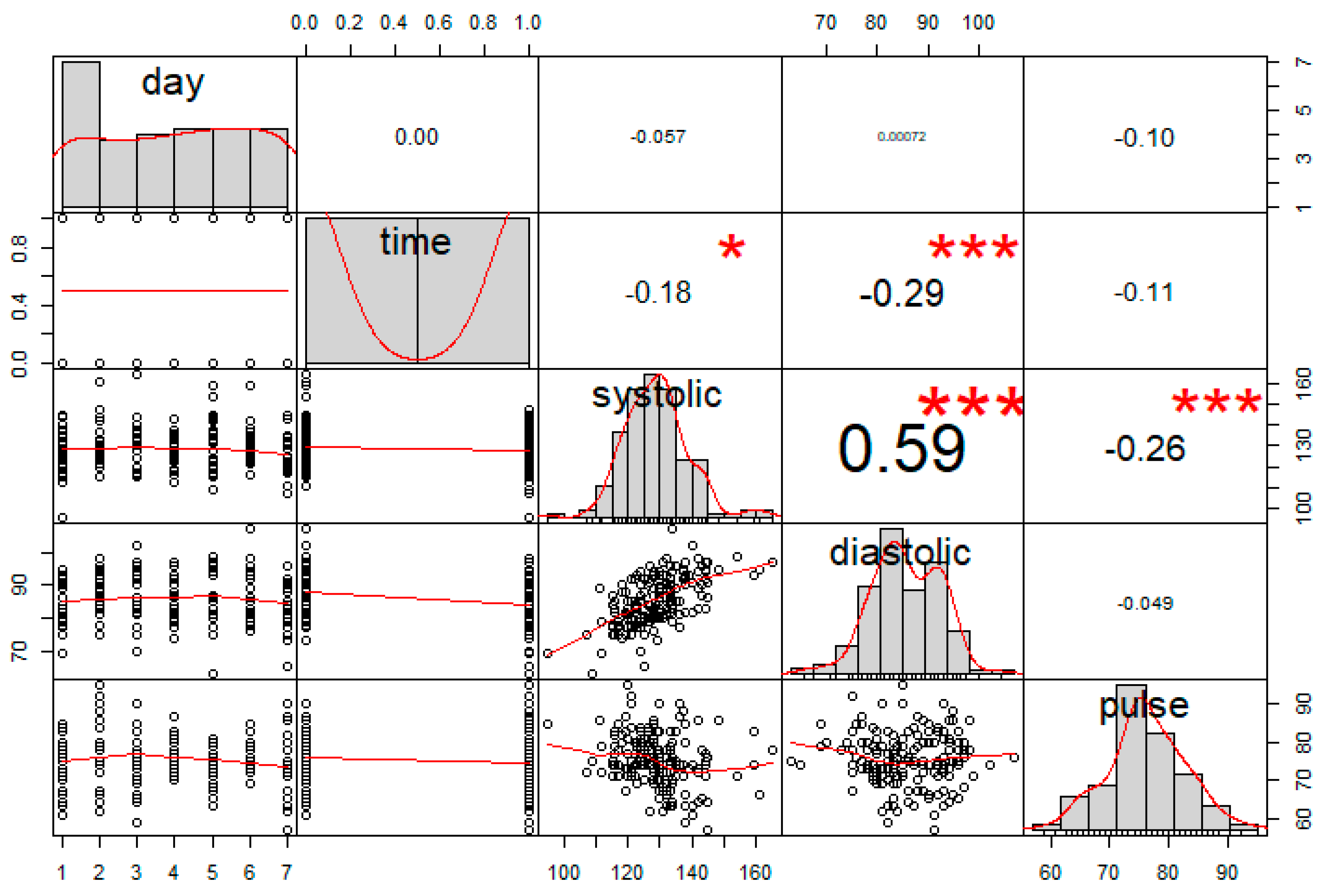
Blood pressure (BP) is one of the main risk factors for cardiovascular diseases. BP is the force of blood pushing against your artery walls as it goes through your body [16]. Abnormal BP has been a forceful issue that causes strokes, heart attacks, and kidney failureso it is important to check your blood pressure on a regular basis. The author has monitored blood pressure daily of an individual since January 2019 using Microlife product. He measured his blood pressure each morning and evening each day within the same time interval and recorded the results of all three measures such as Systolic Blood Pressure ("systolic"), Diastolic Blood Pressure ("diastolic"), and Heart Rate ("pulse") each time as shown in

Table 9. Sample heart blood pressure health data set of an individual in 86-day interval.

Day	Time	Systolic	Diastolic	Pulse
5	0	154	99	71
5	1	144	94	75
6	0	139	93	73
6	1	128	76	85
7	0	129	73	78
7	1	125	65	74
1	0	129	80	70
1	1	130	83	72
2	0	144	83	74
2	1	124	87	84
3	0	120	77	73
3	1	124	70	80

. The Systolic BP is the pressure when the heart beats – while the heart muscle is contracting (squeezing) and pumping oxygen-rich blood into the blood vessels. Diastolic BP is the pressure on the blood vessels when the heart muscle relaxes. The diastolic pressure is always lower than the systolic pressure [17]. The Pulse or Heart rate measures the heart rate by counting the number of beats per minute (BPM).

The newly heart blood pressure health data set consists of the heart rate (pulse) of such individual in 86 days with 2 data points measured each day, making a total of 172 observations. The first few rows of the data set are shown in Table 9. In Table 9 for example, the first row of the data set can be read as follows: on a Thursday ("day" = 5) morning ("time"=0), the high blood "systolic", low blood "diastolic", and heart rate "pulse" measurements were 154, 99, and 71, respectively. Similarly, on a Thursday afternoon (i.e., the second row of the data set in Table 9, and "time" =1), the high blood, low blood and heart rate measurements were 144, 94, and 75, respectively.

From Figure 3, the systolic BP and diastolic BP have the highest correlation. In this study, we decided not to include the Time variable (i.e., column 2 in Table 9) in this model analysis since it may not necessary reflect the health measurement much. The analysis shows that the Systolic blood pressure seems to be the most significant factor that can have strong impacts on the heart rate measure. The R² is 0.09997, so 9.99% of the variability is explained by all three variables (Day, Systolic, Diastolic) as shown in

Table 10. Criteria values of variables (day, systolic, diastolic) of regression models (X₁, X₂, and X₃ be denoted as the day, systolic, diastolic, respectively).

Criteria	X1, X2, X3	X1, X2	X1, X3	X2, X3	X1	X2	X3
MSE	43.1175	43.7381	47.0101	43.5859	46.8450	44.1352	47.2311
AIC	1141.463	1142.942	1155.351	1142.342	1153.76	1143.511	1155.172
BIC	1154.053	1152.384	1164.793	1151.784	1160.055	1149.806	1161.467
RMSE	6.5664	6.6135	6.8564	6.6020	6.8443	6.6434	6.8725
R2	0.09997	0.0816	0.01287	0.08477	0.0105	0.0678	0.00236
Adjusted R2	0.08389	0.0707	0.00119	0.07394	0.00469	0.0623	−0.00351
PIC	10.6378	9.6490	9.8919	9.6375	8.8561	8.6552	8.8843

. Based on the new proposed criterion, the model with only Systolic blood pressure variable is the best model from the set of seven candidate models as shown in Table 10. This result stands alone compared to all other criteria, except BIC. In other words, the best model based on our proposed criterion will only obtain Systolic BP variable in the model.

Application 3: Software Reliability Dataset #1.

In this example, we use the numerical results recently studied by Song et al. [12] to illustrate the new criterion by comparing it to some existing criteria based on the two real data sets in the applications of software reliability engineering.

Table 11. Results for criteria based on dataset #1 [12].

No.	Value k	Model	MSE	AIC	R2	Adj R2	PIC
1	2	GO	3.6343	62.8309	0.9687	0.9630	45.7783
2	2	DS	9.1885	68.6375	0.9208	0.9064	112.4287
3	3	IS	3.9647	64.8309	0.9687	0.9593	47.1572
4	4	YE	4.1162	66.7083	0.9704	0.9573	46.3621
5	4	YR	16.0972	82.0186	0.8844	0.8331	166.1721
6	3	YID1	2.9149	64.8745	0.9770	0.9701	35.6094
7	3	YID2	2.9795	64.7603	0.9765	0.9694	36.3199
8	3	HDGO	3.9647	64.8309	0.9687	0.9593	47.1572
9	4	PNZ	3.2378	66.6674	0.9768	0.9664	37.5782
10	5	PZ	4.8458	68.8309	0.9687	0.9491	50.8344
11	6	ZFR	5.4529	70.8319	0.9687	0.9418	53.3732
12	5	TP	5.2511	72.6973	0.9736	0.9428	54.4821
13	3	IFD	13.0533	67.8928	0.8969	0.8660	147.132
14	4	PDP	26.2542	138.4862	0.8115	0.7277	267.742
15	4	KSRGM	5.3204	65.7919	0.9618	0.9448	58.4041
16	4	RMD	3.3303	66.7588	0.9761	0.9655	38.5032
17	5	CT	4.0547	68.0606	0.9738	0.9574	43.7145
18	5	Vtub	3.7733	66.2648	0.9756	0.9604	41.1819
19	5	3PFD	4.3488	68.6419	0.9719	0.9543	46.3614

shows the numericalresults of 19 different software reliability models based on four existing criteria such as MSE, AIC, R², and adjusted R² and a new criterion, called Pham criterion, using dataset #1 [18]. In dataset #1, the week index ranges from 1 week to 21 weeks, and there are 38 cumulative failures at 14 weeks. Detailed information is recorded in Musa et al. [18]. Model 6 as shown in Table 11 provides the best fit based on the MSE, R², adjusted R² and new criteria. However, Model 1 seems to be the best fit based on the AIC.

Application 4: Software Reliability based on Dataset #2.

Similarly, in this example we use the numerical results recently studied by Song et al. [12] to illustrate the new criterion based on a real dataset #2 [19]. In dataset #2, the weekly index uses cumulative system days, and the failures in 58,633 system days. The detailed information is recorded in [19].

Table 12. Results for criteria based on dataset #2 [12].

No.	Value k	Model	MSE	AIC	R2	Adj R2	PIC
1	2	GO	1.6266	49.4070	0.9839	0.9806	20.0744
2	2	DS	7.3713	72.2378	0.9269	0.9122	83.2661
3	3	IS	1.7892	51.4070	0.9839	0.9785	21.4920
4	4	YE	1.9812	53.3655	0.9839	0.9759	23.1641
5	4	YR	2.8131	91.6713	0.8960	0.8440	120.6512
6	3	YID1	1.0219	48.4929	0.9908	0.9877	13.8190
7	3	YID2	0.9979	48.4804	0.9910	0.9880	13.5790
8	3	HDGO	1.7883	51.3850	0.9839	0.9785	21.4830
9	4	PNZ	1.1090	50.4830	0.9910	0.9865	15.3143
10	5	PZ	1.3039	53.3626	0.9906	0.9839	17.9312
11	6	ZFR	2.5591	57.3622	0.9838	0.9677	28.4794
12	5	TP	1.3344	56.0182	0.9928	0.9827	18.1752
13	3	IFD	38.8383	65.7427	0.6497	0.5330	391.983
14	4	PDP	34.4540	134.4592	0.7203	0.5805	351.4193
15	4	KSRGM	3.2468	55.0954	0.9736	0.9605	34.5545
16	4	RMD	2.0411	53.5239	0.8934	0.9751	23.7032
17	5	CT	0.9229	51.9769	0.9933	0.9886	14.8832
18	5	Vtub	2.0950	52.9672	0.9849	0.9741	24.2600
19	5	3PFD	1.2405	52.9005	0.9910	0.9847	17.4241

presents the numerical results of 19 different software reliability models based on four existing criteria such as MSE, AIC, R², and adjusted R² and the new proposed criterion.

Based on dataset #2, Model 7 (see Table 12) provides the best fit based on the AIC and new criteria where Model 17 indicates to be the best fit based on the MSE, R², and adjusted R².

4. Conclusions

In this paper we proposed a new PIC that can be used to select the best model from a set of candidate models. The proposed criterion takes into account a larger penalty when adding too many coefficients (or estimated parameters) in the model from too small a sample in the presence of too much noise where n is the sample size and k is the number of estimated parameters.

The paper illustrates the proposed criterion with several applications based on the Advertising budget data, the newly Heart Blood Pressure Health dataset, and software failure data. Given the number of estimated parameters k and sample size n, it is straightforward to obtain the new criterion value. Based on the three real applications studied in this paper, PIC has a very attractive performance which is accuracy based on both simulated data and several real world applications discussed in Section 3 for selecting the best model among a set of candidates.

References

- Burnham, K.P.; Anderson, D.R. Model Selection and Multimodel Inference: A Practical Information-Theoretic Approach, 2nd ed.; Springer: Berlin, Germany, 2002. [Google Scholar]
- Burnham, K.P.; Anderson, D.R. Multimodel inference: Understanding AIC and BIC in model selection. Sociol. Methods Res. 2004, 33, 261–304. [Google Scholar] [CrossRef]
- Burnham, K.P.; Anderson, D.R.; Huyvaert, K.P. AIC model selection and multimodel inference in behavioral ecology: Some background, observations, and comparisons. Behav. Ecol. Sociobiol. 2011, 65, 23–35. [Google Scholar] [CrossRef]
- Guyon, I.; Elisseeff, A. An introduction to variable and feature selection. J. Mach. Learn. Res. 2003, 3, 1157–1182. [Google Scholar]
- Akaike, H. Information theory and an extension of the maximum likelihood principle. In Proceedings of the Second International Symposium on Information Theory; Petrov, B.N., Caski, F., Eds.; AkademiaiKiado: Budapest, Hungary, 1973; pp. 267–281. [Google Scholar]
- Allen, D.M. Mean square error of prediction as a criterion for selecting variables. Technometrics. 1971, 13, 469–475. [Google Scholar] [CrossRef]
- Bozdogan, H. Akaike’s Information criterion and recent developments in information complexity. J. Math. Psychol. 2000, 44, 62–91. [Google Scholar] [CrossRef] [PubMed] [Green Version]
- Chai, T.; Draxler, R.R. Root mean square error (RMSE) or mean absolute error (MAE)? Arguments against avoiding RMSE in the literature. Geosci. Model Dev. 2014, 7, 1247–1250. [Google Scholar] [CrossRef] [Green Version]
- Schönbrodt, F.D.; Wagenmakers, E.-J. Bayes factor design analysis: Planning for compelling evidence. Psychon. Bull. Rev. 2017, 25, 128–142. [Google Scholar] [CrossRef] [PubMed]
- Schwarz, G. Estimating the dimension of a model. Ann. Stat. 1978, 6, 461–464. [Google Scholar] [CrossRef]
- Wagenmakers, E.-J.; Farrell, S. AIC model selection using Akaike weights. Psychon. Bull. Rev. 2004, 11, 192–196. [Google Scholar] [CrossRef] [PubMed]
- Song, K.Y.; Chang, I.-H.; Pham, H. A testing coverage model based on NHPP software reliability considering the software operating environment and the sensitivity analysis. Mathematics 2019, 7, 450. [Google Scholar] [CrossRef] [Green Version]
- Pham, H. System Software Reliability; Springer: London, UK, 2006. [Google Scholar]
- Li, Q.; Pham, H. A testing-coverage software reliability model considering fault removal efficiency and error generation. PloS ONE 2017, 12, e0181524. [Google Scholar] [CrossRef] [PubMed] [Green Version]
- Advertising Budgets Data Set. Available online: https://www.kaggle.com/ishaanv/ISLR-Auto#Advertising.csv (accessed on 30 May 2019).
- Blood Pressure. Available online: https://www.webmd.com/hypertension-high-blood-pressure/guide/hypertension-home-monitoring#1 (accessed on 30 April 2019).
- Systolic. Available online: https://0-www-ncbi-nlm-nih-gov.brum.beds.ac.uk/books/NBK279251/ (accessed on 30 April 2019).
- Musa, J.D.; Iannino, K.; Okumoto, K. Software Reliability Measurement Prediction Application; McGraw-Hill: New York, NY, USA, 2006. [Google Scholar]
- Daniel, R.J.; Zhang, X. Some successful approaches to software reliability modeling in industry. J. Syst. Softw. 2005, 74, 85–99. [Google Scholar]
Figure 1.
The scatter plot of the advertising data with four variables.
Figure 2.
The correlation coefficient between the variables.
Figure 3.