Cost-Based Optimum Design of Reinforced Concrete Retaining Walls Considering Different Methods of Bearing Capacity Computation


Abstract
:1. Introduction
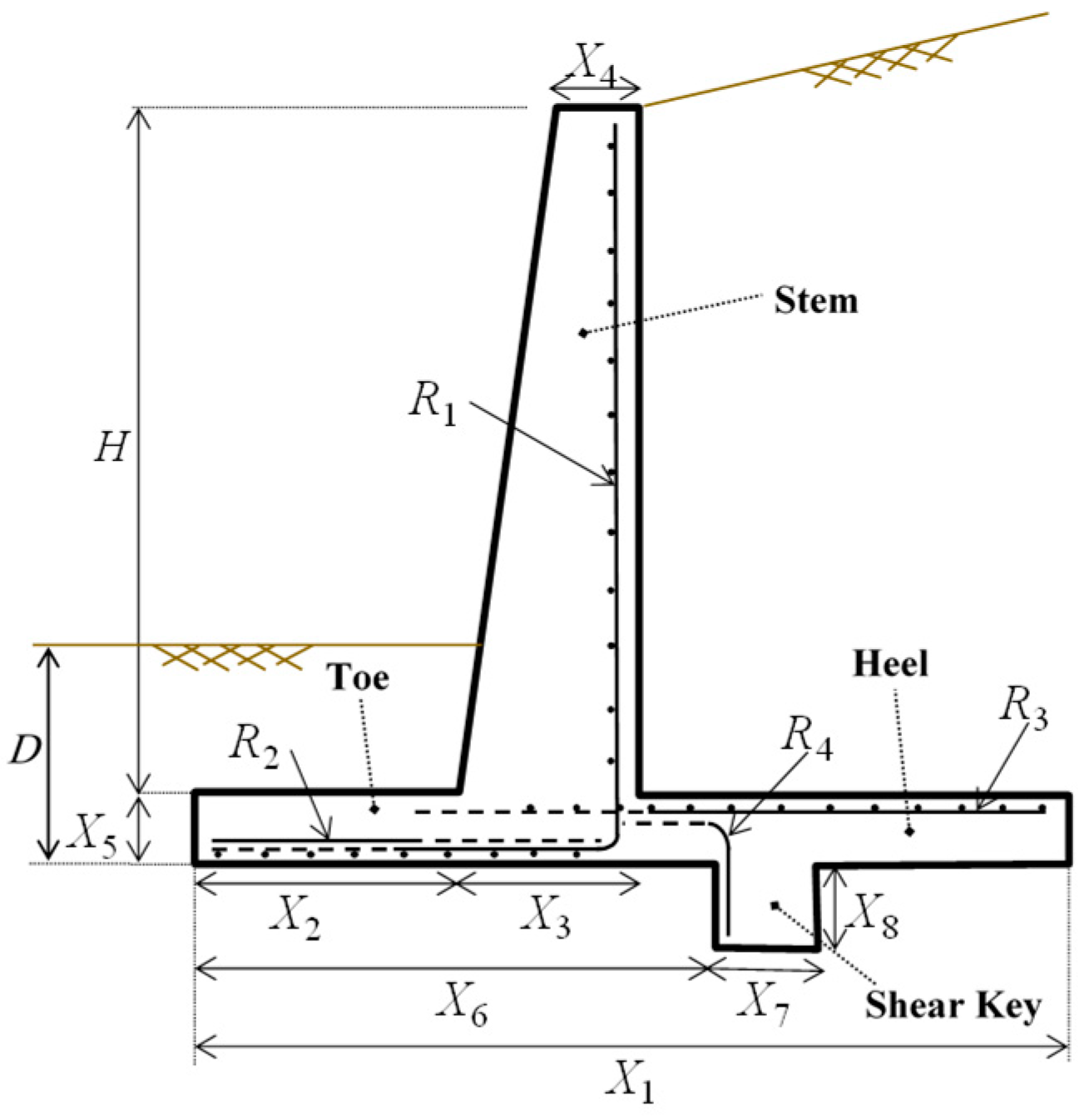
2. Design of Retaining Walls
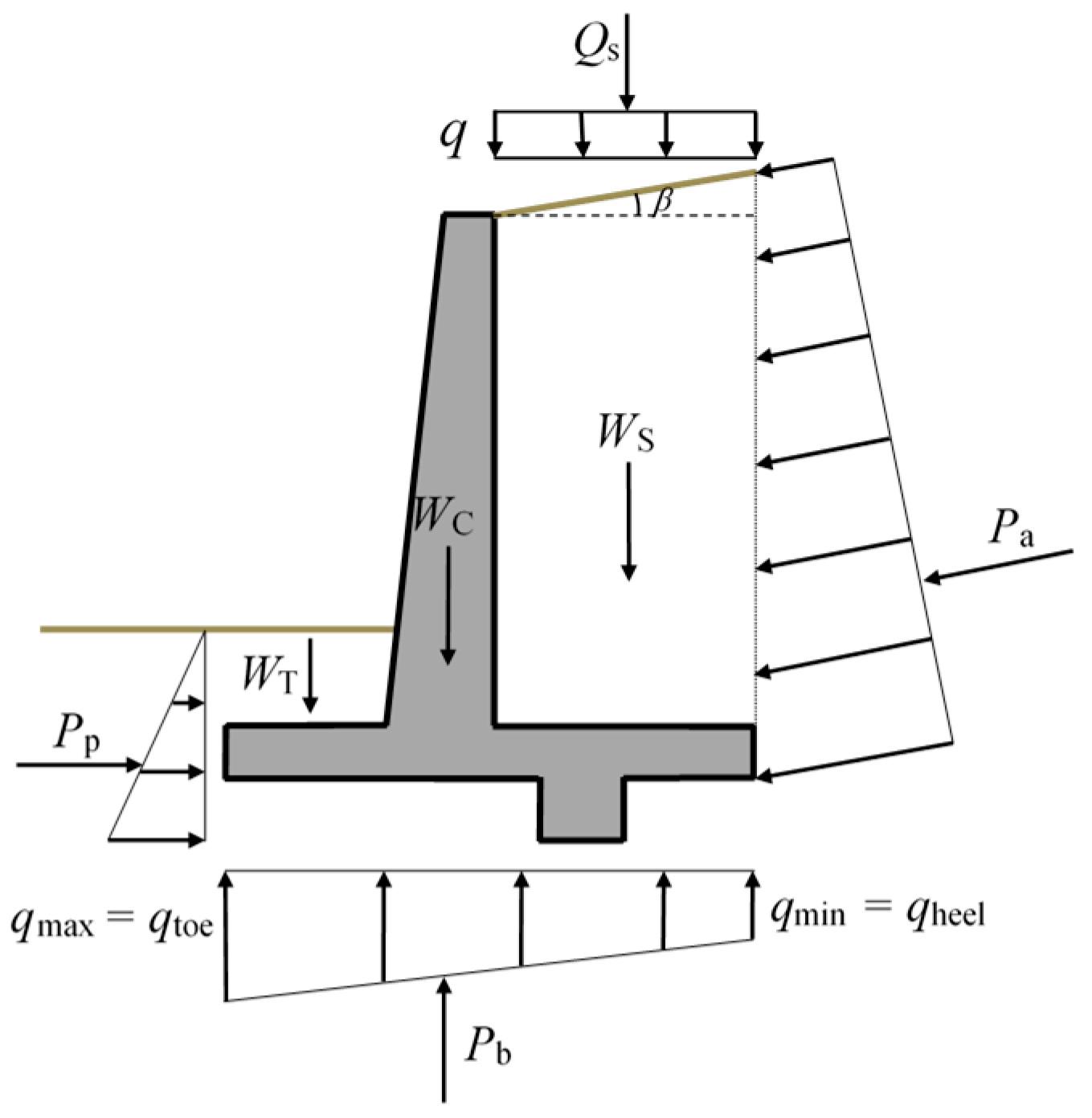
2.1. Geotechnical Stability Demands
2.2. Structural Requirements
2.2.1. Flexural Moment and Shear Force Demands of Stem
2.2.2. Flexural Moment and Shear Force Demands of Toe Slab
2.2.3. Flexural Moment and Shear Force Demands of Heel Slab
3. Optimization Problem
3.1. Formulation
3.2. Objective Function
3.3. Design Constraints
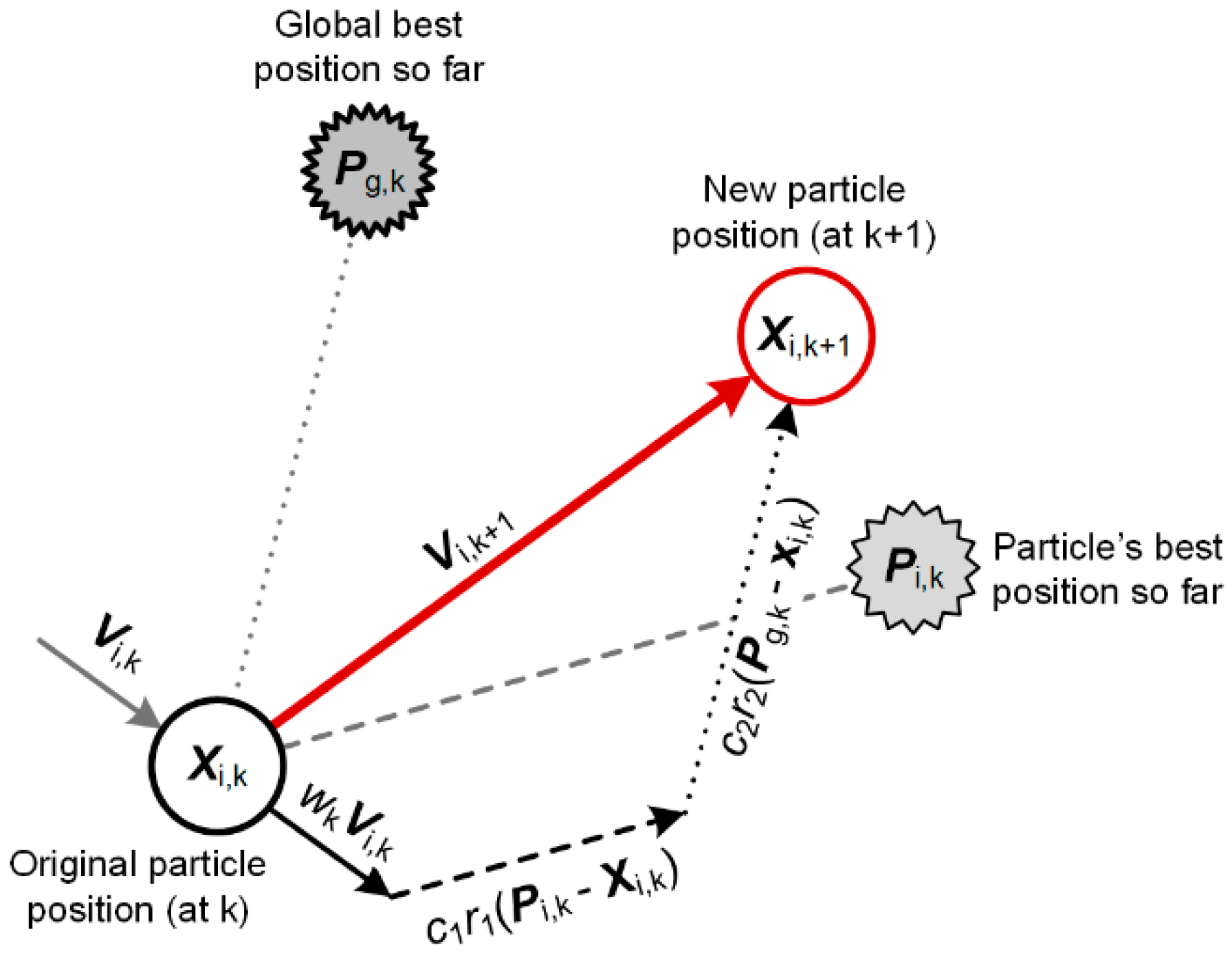
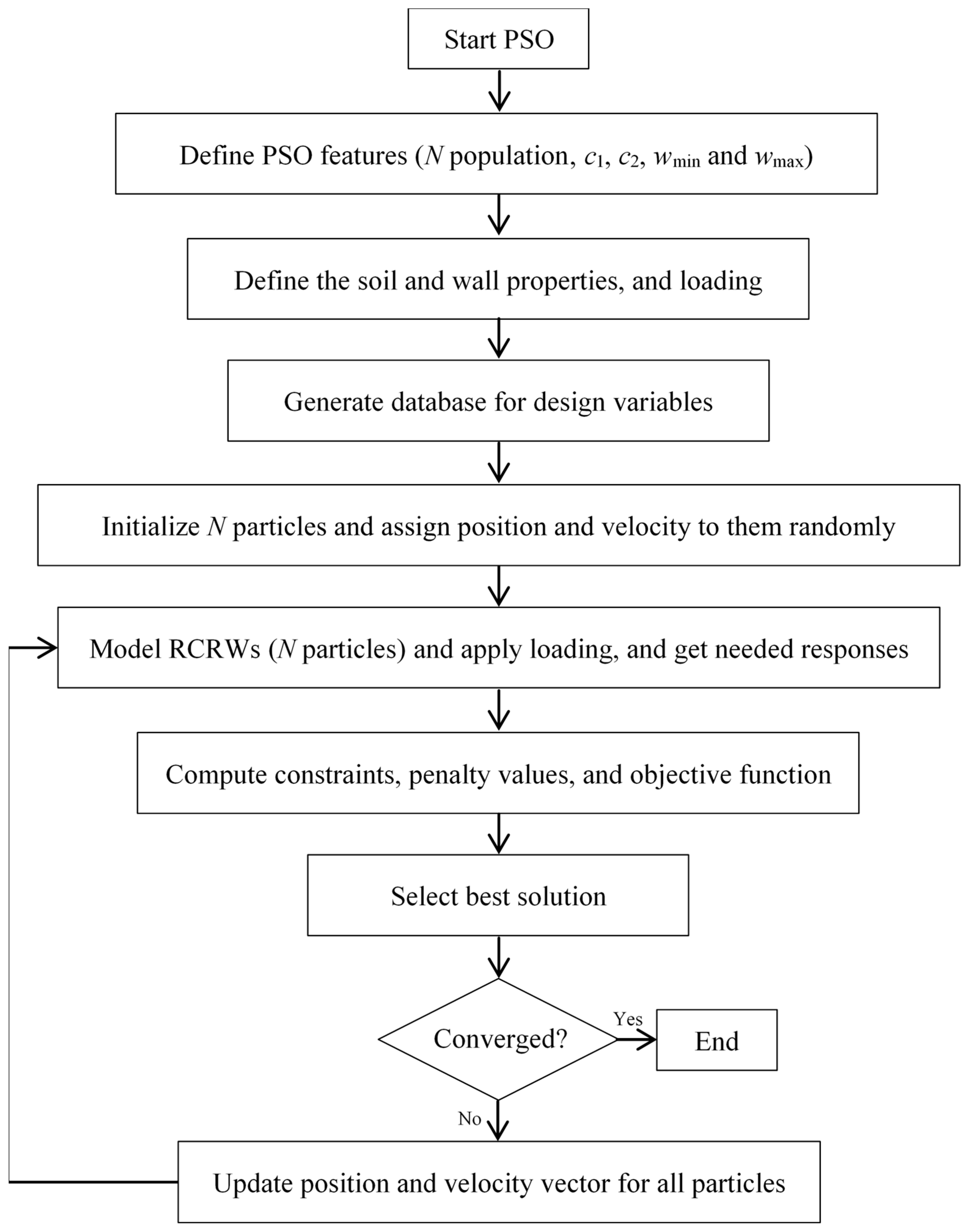
3.4. PSO Algorithm
4. Methodology
5. Design Examples
5.1. Assumptions
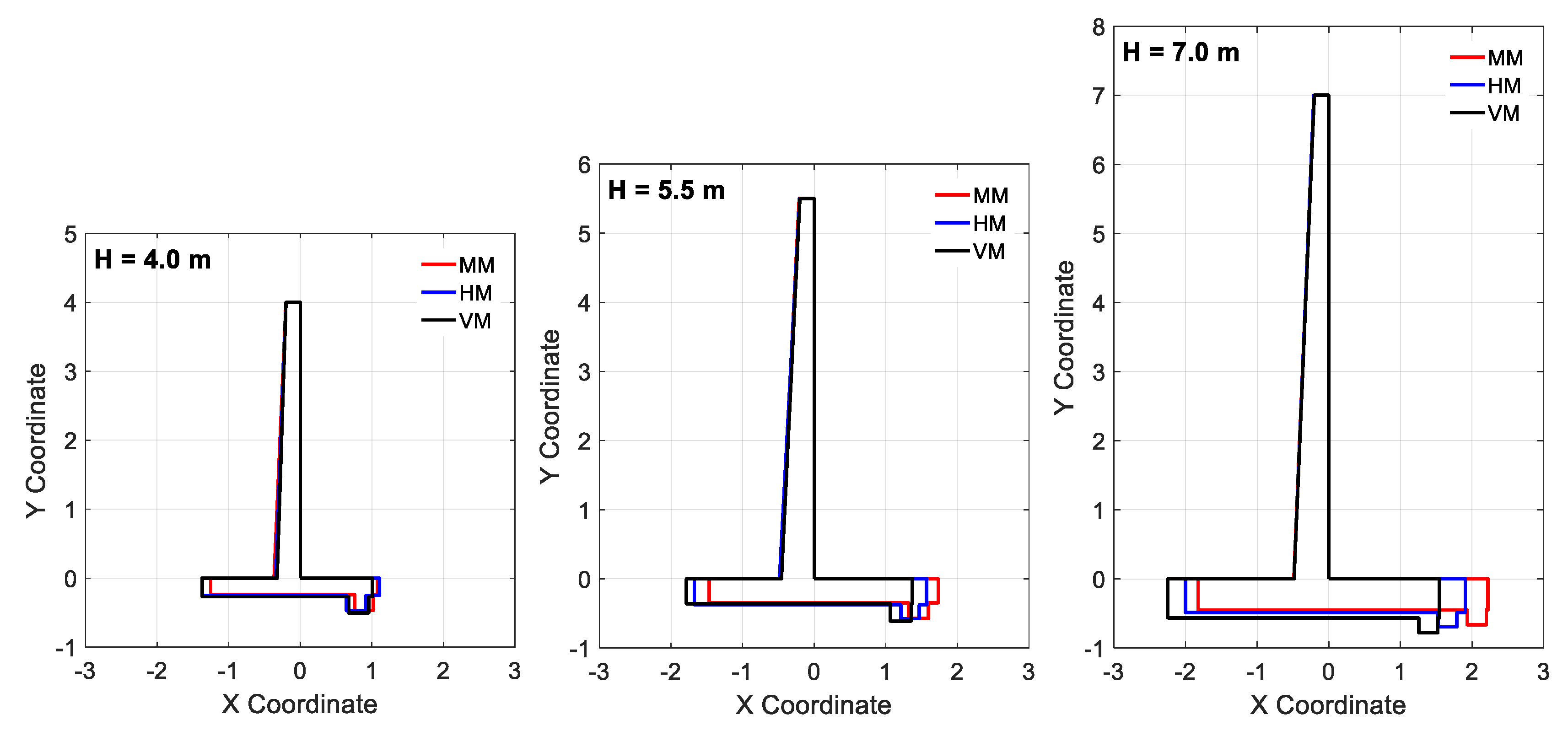
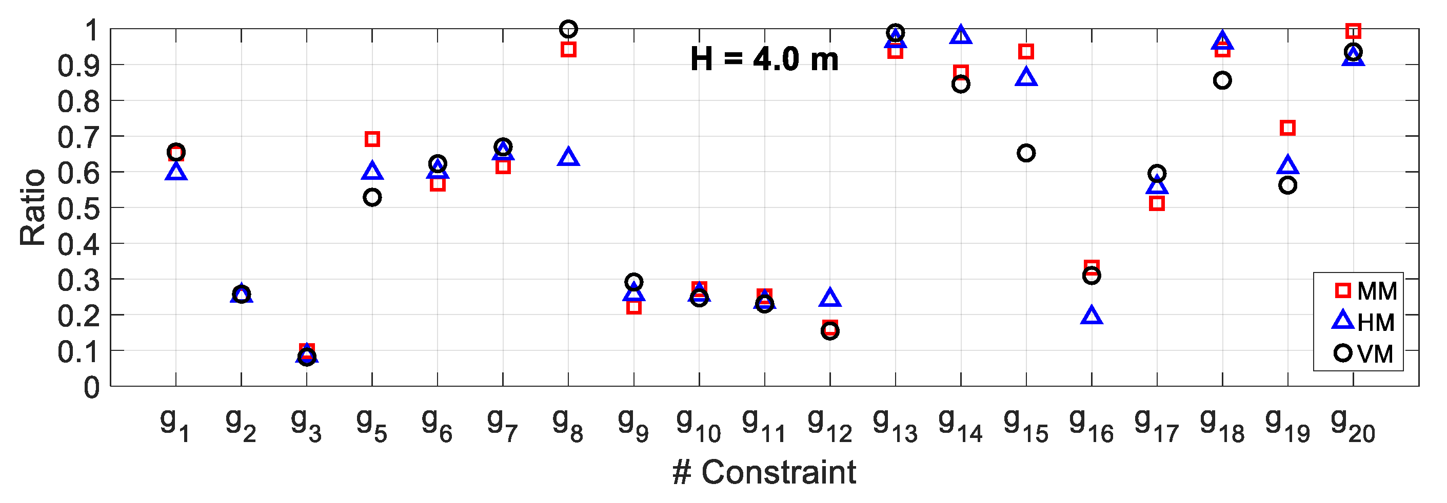
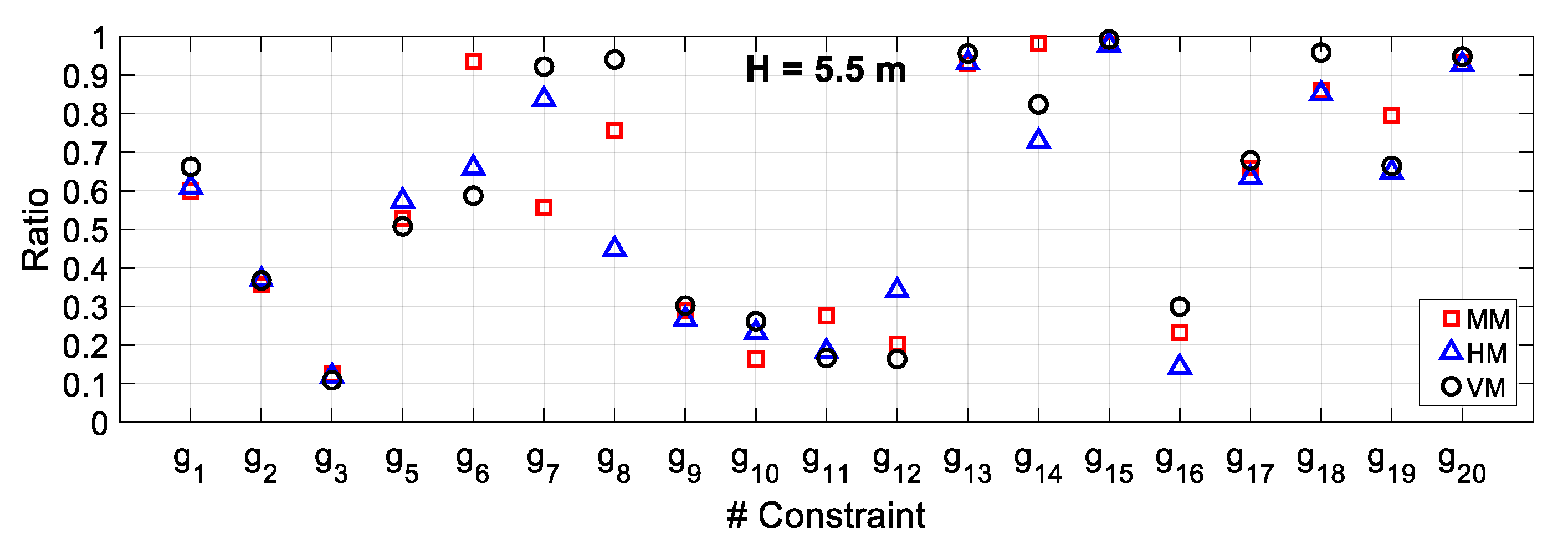
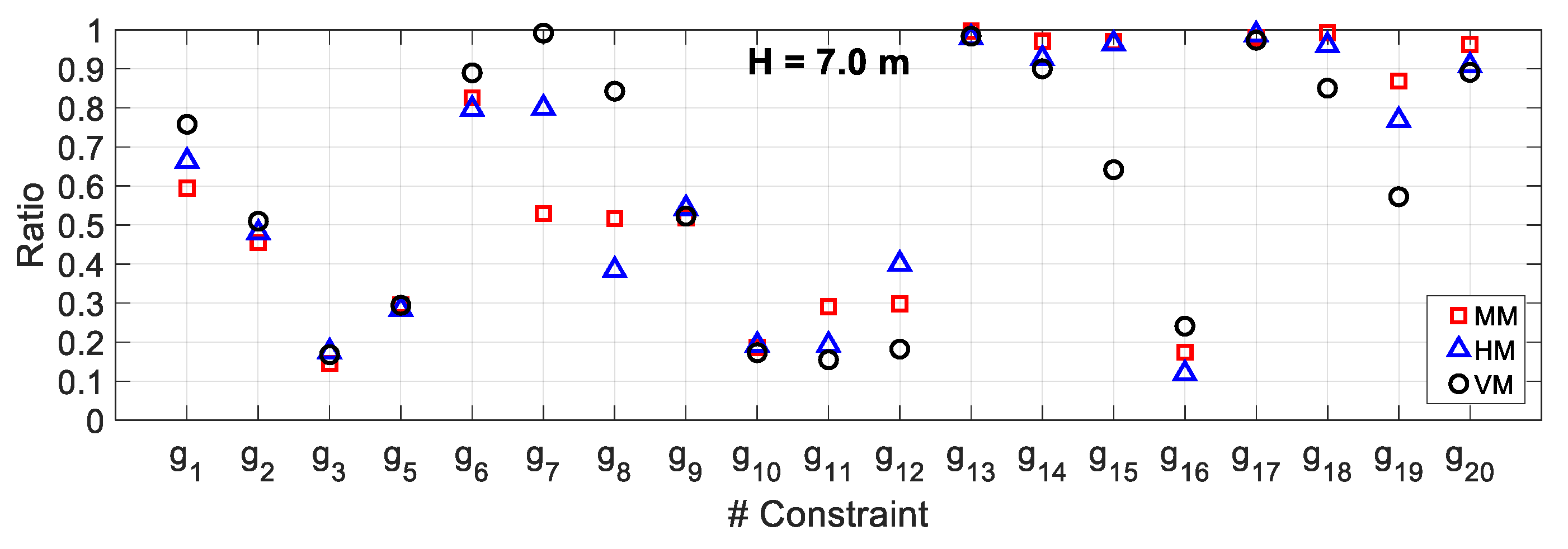
5.2. Results and Discussion
5.3. Comparative Study
5.4. Effect of Backfill Slope
5.5. Effect of Surcharge Load
6. Conclusions
Author Contributions
Funding
Conflicts of Interest
Appendix A

References
- Sarıbaş, A.; Erbatur, F. Optimization and sensitivity of retaining structures. J. Geotech. Eng. 1996, 122, 649–656. [Google Scholar] [CrossRef]
- Ceranic, B.; Fryer, C.; Baines, R. An application of simulated annealing to the optimum design of reinforced concrete retaining structures. Comput. Struct. 2001, 79, 1569–1581. [Google Scholar] [CrossRef] [Green Version]
- Víctor, Y.; Julian, A.; Cristian, P.; Fernando, G.-V. A parametric study of optimum earth-retaining walls by simulated annealing. Eng. Struct. 2008, 30, 821–830. [Google Scholar]
- Camp, C.V.; Akin, A. Design of retaining walls using big bang–big crunch optimization. J. Struct. Eng. 2011, 138, 438–448. [Google Scholar] [CrossRef]
- Khajehzadeh, M.; Taha, M.R.; El-Shafie, A.; Eslami, M. Economic design of retaining wall using particle swarm optimization with passive congregation. Aust. J. Basic Appl. Sci. 2010, 4, 5500–5507. [Google Scholar]
- Gandomi, A.H. Optimization of retaining wall design using recent swarm intelligence techniques. Eng. Struct. 2015, 103, 72–84. [Google Scholar] [CrossRef]
- Kaveh, A.; Khayatazad, M. Optimal design of cantilever retaining walls using ray optimization method. Iranian Journal of Science and Technology. Trans. Civ. Eng. 2014, 38, 261. [Google Scholar]
- Kaveh, A.; Soleimani, N. CBO and DPSO for optimum design of reinforced concrete cantilever retaining walls. Asian J. Civ. Eng. 2015, 16, 751–774. [Google Scholar]
- Kaveh, A.; Farhoudi, N. Dolphin echolocation optimization for design of cantilever retaining walls. Asian J. Civ. Eng. 2016, 17, 193–211. [Google Scholar]
- Kaveh, A.; Laien, D.J. Optimal design of reinforced concrete cantilever retaining walls using CBO, ECBO and VPS algorithms. Asian J. Civ. Eng. 2017, 18, 657–671. [Google Scholar]
- Temur, R.; Bekdaş, G. Teaching learning-based optimization for design of cantilever retaining walls. Struct. Eng. Mech. 2016, 57, 763–783. [Google Scholar] [CrossRef]
- Ukritchon, B.; Chea, S.; Keawsawasvong, S. Optimal design of Reinforced Concrete Cantilever Retaining Walls considering the requirement of slope stability. KSCE J. Civ. Eng. 2017, 21, 2673–2682. [Google Scholar] [CrossRef]
- Aydogdu, I. Cost optimization of reinforced concrete cantilever retaining walls under seismic loading using a biogeography-based optimization algorithm with Levy flights. Eng. Optim. 2017, 49, 381–400. [Google Scholar] [CrossRef]
- Kumar, V.N.; Suribabu, C. Optimal design of cantilever retaining wall using differential evolution algorithm. Int. J. Optim. Civ. Eng. 2017, 7, 433–449. [Google Scholar]
- Gandomi, A.; Kashani, A.; Zeighami, F. Retaining wall optimization using interior search algorithm with different bound constraint handling. Int. J. Numer. Anal. Methods Geomech. 2017, 41, 1304–1331. [Google Scholar] [CrossRef]
- Gandomi, A.H.; Kashani, A.R. Automating pseudo-static analysis of concrete cantilever retaining wall using evolutionary algorithms. Measurement 2018, 115, 104–124. [Google Scholar] [CrossRef]
- Mergos, P.E.; Mantoglou, F. Optimum design of reinforced concrete retaining walls with the flower pollination algorithm. Struct. Multidiscip. Optim. 2019, 1–11. [Google Scholar] [CrossRef]
- MATLAB. The Language of Technical Computing; Math Works Inc.: Natick, MA, USA, 2005; Volume 2018a. [Google Scholar]
- Kennedy, J.; Eberhart, R. Particle swarm optimization (PSO). In Proceedings of the IEEE International Conference on Neural Networks, Perth, Australia, 27 November–1 December 1995. [Google Scholar]
- ACI. American Concrete Institute: Building Code Requirements for Structural Concrete and Commentary; ACI: Farmington Hills, MI, USA, 2014. [Google Scholar]
- Das, B.M. Principles of Foundation Engineering; Cengage Learning: Boston, MA, USA, 2015. [Google Scholar]
- Meyerhof, G.G. Some recent research on the bearing capacity of foundations. Can. Geotech. J. 1963, 1, 16–26. [Google Scholar] [CrossRef]
- Hansen, J.B. A Revised and Extended Formula for Bearing Capacity; Danish Geotechnical Institute: Lyngby, Denmark, 1970. [Google Scholar]
- Vesic, A.S. Analysis of ultimate loads of shallow foundations. J. Soil Mech. Found. Div. 1973, 99, 45–73. [Google Scholar] [CrossRef]
- Arora, J.S. Introduction to Optimum Design; Elsevier: Amsterdam, The Netherlands, 2004. [Google Scholar]
- Gharehbaghi, S.; Khatibinia, M. Optimal seismic design of reinforced concrete structures under time-history earthquake loads using an intelligent hybrid algorithm. Earthq. Eng. Eng. Vib. 2015, 14, 97–109. [Google Scholar] [CrossRef]
- Gholizadeh, S.; Salajegheh, E. Optimal design of structures subjected to time history loading by swarm intelligence and an advanced metamodel. Comput. Methods Appl. Mech. Eng. 2009, 198, 2936–2949. [Google Scholar] [CrossRef]
- Plevris, V.; Papadrakakis, M. A hybrid particle swarm-gradient algorithm for global structural optimization. Comput.-Aided Civ. Infrastruct. Eng. 2011, 26, 48–68. [Google Scholar] [CrossRef]
- Gholizadeh, S. Layout optimization of truss structures by hybridizing cellular automata and particle swarm optimization. Comput. Struct. 2013, 125, 86–99. [Google Scholar] [CrossRef]
- Yazdani, H. Probabilistic performance-based optimum seismic design of RC structures considering soil–structure interaction effects. ASCE-ASME J. Risk Uncertain. Eng. Syst. Part A Civ. Eng. 2016, 3, G4016004. [Google Scholar] [CrossRef]
- Gharehbaghi, S.; Moustafa, A.; Salajegheh, E. Optimum seismic design of reinforced concrete frame structures. Comput. Concr. 2016, 17, 761–786. [Google Scholar] [CrossRef]
- Gharehbaghi, S. Damage controlled optimum seismic design of reinforced concrete framed structures. Struct. Eng. Mech. 2018, 65, 53–68. [Google Scholar]
- Khatibinia, M.; Jalali, M.; Gharehbaghi, S. Shape optimization of U-shaped steel dampers subjected to cyclic loading using an efficient hybrid approach. Eng. Struct. 2019, 197, 108874. [Google Scholar] [CrossRef]


| Geometric Variable | Description | Lower Bound | Upper Bound |
|---|---|---|---|
| X1 | Width of the base slab | 0.4H | 0.8H |
| X2 | Toe width | 0.1H | 0.6H |
| X3 | Thickness at the bottom of the stem | 0.2 m | 0.5 m |
| X4 | Thickness at the top of the stem | 0.2 m | 0.4 m |
| X5 | Thickness of the base | 0.2 m | 0.3H |
| X6 | Distance from the toe to the front face of the shear key | 0.5H | 0.8H |
| X7 | Width of shear key | 0.2 m | 0.4 m |
| X8 | Depth of the shear key | 0.2 m | 0.9 m |
| Reinforcement Variable | Description |
|---|---|
| R1 | Vertical steel reinforcement of the stem |
| R2 | Horizontal steel reinforcement of the toe |
| R3 | Horizontal steel reinforcement of the heel |
| R4 | Vertical steel reinforcement of shear key |
| Index Number | Bars Quantity and Size (R) | Bars Cross-Sectional Area (cm2) (in Ascending Order) |
|---|---|---|
| 1 | 3ϕ10 | 2.356 (lower bound) |
| 2 | 4ϕ10 | 3.141 |
| 3 | 3ϕ12 | 3.392 |
| 4 | 5ϕ10 | 3.926 |
| 5 | 4ϕ12 | 4.523 |
| . | . | . |
| . | . | . |
| 221 | 16ϕ30 | 113.097 |
| 222 | 17ϕ30 | 120.165 |
| 223 | 18ϕ30 | 127.234 (upper bound) |
| Parameter | Symbol | Value | Unit |
|---|---|---|---|
| Examples 1–3 | |||
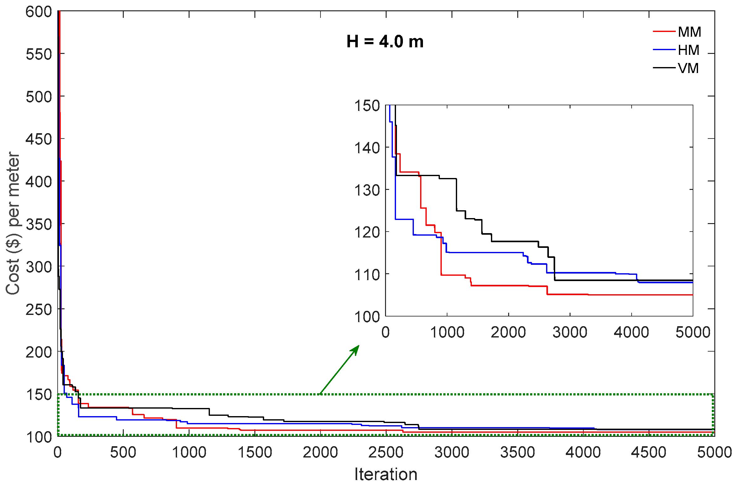
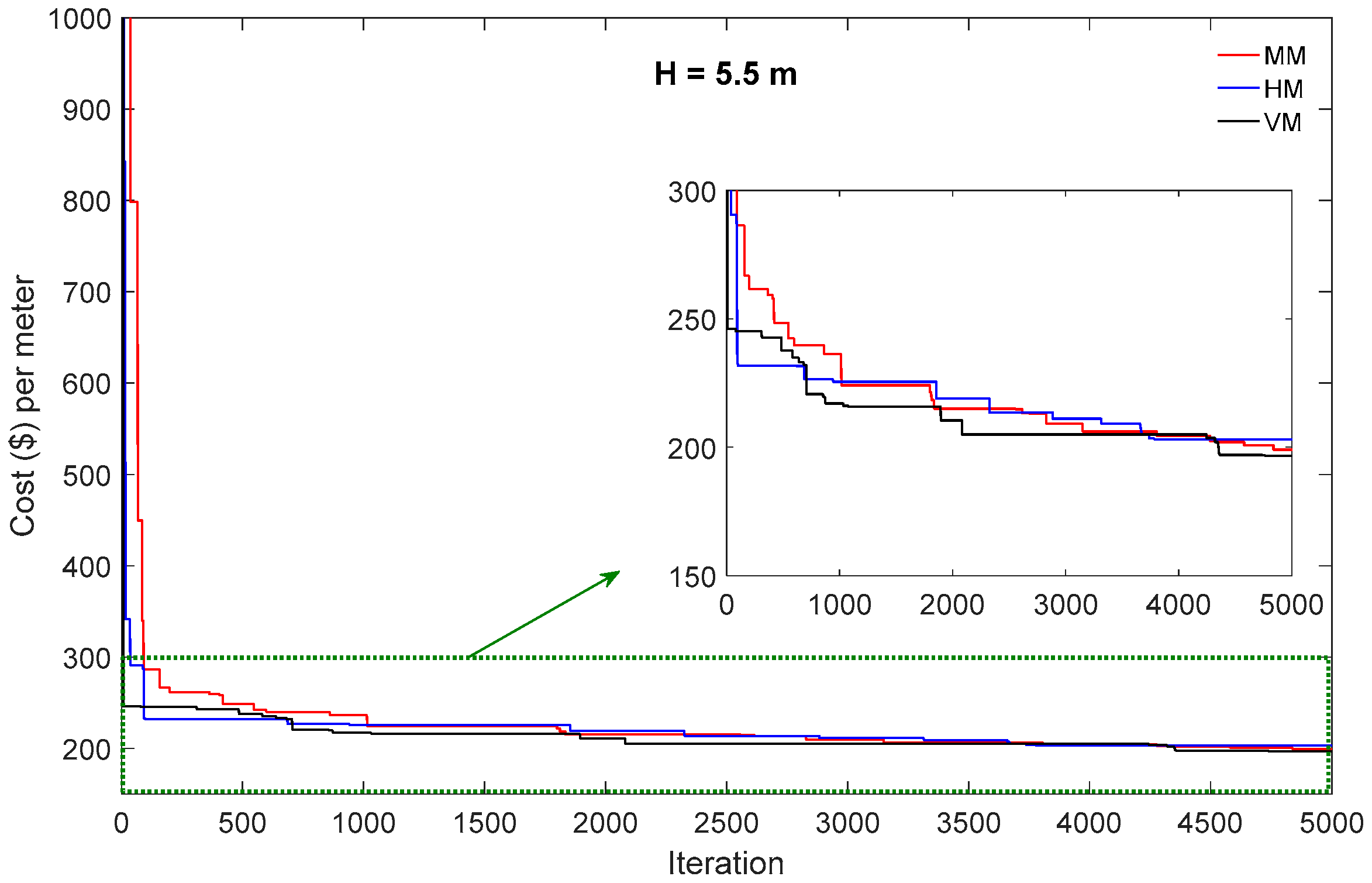
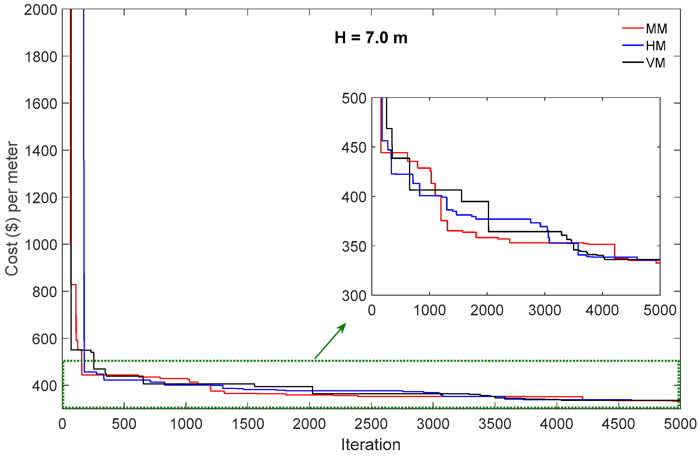
| Height of stem | H | 4.0, 5.5, and 7.0 | m |
| Steel yield strength | fy | 400 | MPa |
| Shrinkage and temperature reinforcement ratio | ρst | 0.002 | - |
| Concrete compressive strength | fc | 21 | MPa |
| Concrete cover | CC | 7 | cm |
| Unit weight of concrete | γc | 23.5 | kN/m3 |
| Unit weight of steel bars | γs | 78.5 | kN/m3 |
| Surcharge load | q | 15 | kPa |
| Backfill slope | β | 5 | degrees |
| Internal friction angle of backfill | φrs | 36 | degrees |
| Unit weight of backfill | γrs | 17.5 | kN/m3 |
| Internal friction angle of base soil | φbs | 39 | degrees |
| Cohesion of base soil | cbs | 0 | kPa |
| Unit weight of base soil | γbs | 20 | kN/m3 |
| Embedment depth of the toe | D | 0.75 | m |
| Cost of steel per unit of mass | Cst | 0.4 | $/kg |
| Cost of concrete per unit of volume | Cc | 40 | $/m3 |
| Variable | Method | Difference (%) | |||
|---|---|---|---|---|---|
| MM | HM | VM | 100 × (HM − MM)/MM | 100 × (VM − MM)/MM | |
| X1 | 2.33 | 2.47 | 2.38 | 6.01 | 2.15 |
| X2 | 0.88 | 1.03 | 1.05 | 17.05 | 19.32 |
| X3 | 0.37 | 0.34 | 0.32 | −8.11 | −13.51 |
| X4 | 0.20 | 0.20 | 0.20 | 0.00 | 0.00 |
| X5 | 0.24 | 0.25 | 0.27 | 4.17 | 12.50 |
| X6 | 2.01 | 2.01 | 2.05 | 0.00 | 1.99 |
| X7 | 0.26 | 0.27 | 0.28 | 3.85 | 7.69 |
| X8 | 0.23 | 0.22 | 0.24 | −4.35 | 4.35 |
| R1 | 13ϕ12 | 20ϕ10 | 21ϕ10 | 6.84 | 12.18 |
| R2 | 13ϕ10 | 9ϕ12 | 14ϕ10 | −0.31 | 7.69 |
| R3 | 13ϕ10 | 12ϕ10 | 9ϕ12 | 0.00 | 8.00 |
| R4 | 6ϕ12 | 14ϕ10 | 9ϕ10 | 62.04 | 4.17 |
| Variable | Method | Difference (%) | |||
|---|---|---|---|---|---|
| MM | HM | VM | 100 × (HM − MM)/MM | 100 × (VM − MM)/MM | |
| X1 | 3.20 | 3.24 | 3.16 | 1.25 | −1.25 |
| X2 | 0.99 | 1.19 | 1.33 | 20.20 | 34.34 |
| X3 | 0.47 | 0.48 | 0.46 | 2.13 | −2.13 |
| X4 | 0.21 | 0.20 | 0.20 | −4.76 | −4.76 |
| X5 | 0.35 | 0.38 | 0.36 | 8.57 | 2.86 |
| X6 | 2.78 | 2.88 | 2.85 | 3.60 | 2.52 |
| X7 | 0.28 | 0.26 | 0.29 | −7.14 | 3.57 |
| X8 | 0.23 | 0.20 | 0.25 | −13.04 | 8.70 |
| R1 | 13ϕ16 | 22ϕ12 | 13ϕ16 | −4.81 | 0.00 |
| R2 | 5ϕ16 | 5ϕ20 | 11ϕ14 | 56.25 | 68.44 |
| R3 | 11ϕ14 | 16ϕ10 | 7ϕ14 | −25.79 | −36.36 |
| R4 | 12ϕ10 | 7ϕ16 | 7ϕ12 | 49.33 | −16.00 |
| Variable | Method | Difference (%) | |||
|---|---|---|---|---|---|
| MM | HM | VM | 100 × (HM − MM)/MM | 100 × (VM − MM)/MM | |
| X1 | 4.04 | 3.90 | 3.79 | −3.47 | −6.19 |
| X2 | 1.34 | 1.51 | 1.76 | 12.69 | 31.34 |
| X3 | 0.49 | 0.48 | 0.48 | −2.04 | −2.04 |
| X4 | 0.21 | 0.21 | 0.20 | 0.00 | −4.76 |
| X5 | 0.45 | 0.49 | 0.56 | 8.89 | 24.44 |
| X6 | 3.75 | 3.52 | 3.50 | −6.13 | −6.67 |
| X7 | 0.27 | 0.26 | 0.27 | −3.70 | 0.00 |
| X8 | 0.21 | 0.21 | 0.21 | 0.00 | 0.00 |
| R1 | 19ϕ18 | 11ϕ24 | 19ϕ18 | 2.92 | 0.00 |
| R2 | 14ϕ12 | 16ϕ12 | 17ϕ12 | 14.29 | 21.43 |
| R3 | 16ϕ14 | 23ϕ10 | 22ϕ10 | −26.66 | −29.85 |
| R4 | 5ϕ18 | 22ϕ10 | 7ϕ12 | 35.80 | −37.78 |
| Variable | Example 1—H = 4.0 m | Example 2—H = 5.5 m | Example 3—H = 7.0 m | ||||||
|---|---|---|---|---|---|---|---|---|---|
| MM | HM | VM | MM | HM | VM | MM | HM | VM | |
| qmin | 16.15 | 26.37 | 17.74 | 29.60 | 31.75 | 23.70 | 40.61 | 27.28 | 9.22 |
| Variable | Example 1—H = 4.0 m | Example 2—H = 5.5 m | Example 3—H = 7.0 m | ||||||
|---|---|---|---|---|---|---|---|---|---|
| MM | HM | VM | MM | HM | VM | MM | HM | VM | |
| Concrete ($) | 70.07 | 70.60 | 70.27 | 122.00 | 126.39 | 120.80 | 172.15 | 175.37 | 184.04 |
| Steel ($) | 34.96 | 37.34 | 38.19 | 77.07 | 76.64 | 75.89 | 160.45 | 160.19 | 152.04 |
| Total ($) | 105.04 | 107.94 | 108.46 | 199.08 | 203.03 | 196.68 | 332.61 | 335.56 | 336.08 |
| Diff. (%) to MM for total cost | - | 2.76 | 3.26 | - | 1.99 | −1.20 | - | 0.89 | 1.04 |
| Work | Method | Cost ($/m) |
|---|---|---|
| Gandomi et al. [6] | - | 162.37 |
| This paper | MM | 154.82 |
| HM | 158.13 | |
| VM | 150.49 |
| Method | β (degrees) | |||||
|---|---|---|---|---|---|---|
| 0 | 5 | 10 | 15 | 20 | 25 | |
| MM | 193.52 | 199.08 | 200.78 | 215.98 | 224.86 | 231.04 |
| HM | 195.11 | 203.03 | 197.55 | 212.83 | 221.07 | 240.54 |
| VM | 191.05 | 196.68 | 202.96 | 209.59 | 220.57 | 234.34 |
| HM to MM (Diff. %) | 0.82 | 1.98 | −1.61 | −1.46 | −1.69 | 4.11 |
| VM to MM (Diff. %) | −1.28 | −1.21 | 1.09 | −2.96 | −1.91 | 1.43 |
| Method | q (kPa) | |||||
|---|---|---|---|---|---|---|
| 0 | 5 | 10 | 15 | 20 | 25 | |
| MM | 168.16 | 180.43 | 189.84 | 199.08 | 209.22 | 211.12 |
| HM | 172.47 | 180.88 | 186.93 | 203.03 | 203.69 | 213.82 |
| VM | 175.52 | 179.31 | 188.78 | 196.68 | 204.12 | 214.50 |
| HM to MM (Diff. %) | 2.56 | 0.25 | −1.53 | 1.98 | −2.64 | 1.28 |
| VM to MM (Diff. %) | 4.38 | −0.62 | −0.56 | −1.21 | −2.44 | 1.60 |
© 2019 by the authors. Licensee MDPI, Basel, Switzerland. This article is an open access article distributed under the terms and conditions of the Creative Commons Attribution (CC BY) license (http://creativecommons.org/licenses/by/4.0/).
Share and Cite
Moayyeri, N.; Gharehbaghi, S.; Plevris, V. Cost-Based Optimum Design of Reinforced Concrete Retaining Walls Considering Different Methods of Bearing Capacity Computation. Mathematics 2019, 7, 1232. https://0-doi-org.brum.beds.ac.uk/10.3390/math7121232
Moayyeri N, Gharehbaghi S, Plevris V. Cost-Based Optimum Design of Reinforced Concrete Retaining Walls Considering Different Methods of Bearing Capacity Computation. Mathematics. 2019; 7(12):1232. https://0-doi-org.brum.beds.ac.uk/10.3390/math7121232
Chicago/Turabian StyleMoayyeri, Neda, Sadjad Gharehbaghi, and Vagelis Plevris. 2019. "Cost-Based Optimum Design of Reinforced Concrete Retaining Walls Considering Different Methods of Bearing Capacity Computation" Mathematics 7, no. 12: 1232. https://0-doi-org.brum.beds.ac.uk/10.3390/math7121232