Modeling and Efficiency Optimization of Steam Boilers by Employing Neural Networks and Response-Surface Method (RSM)

 ,
,
Abstract
:1. Introduction
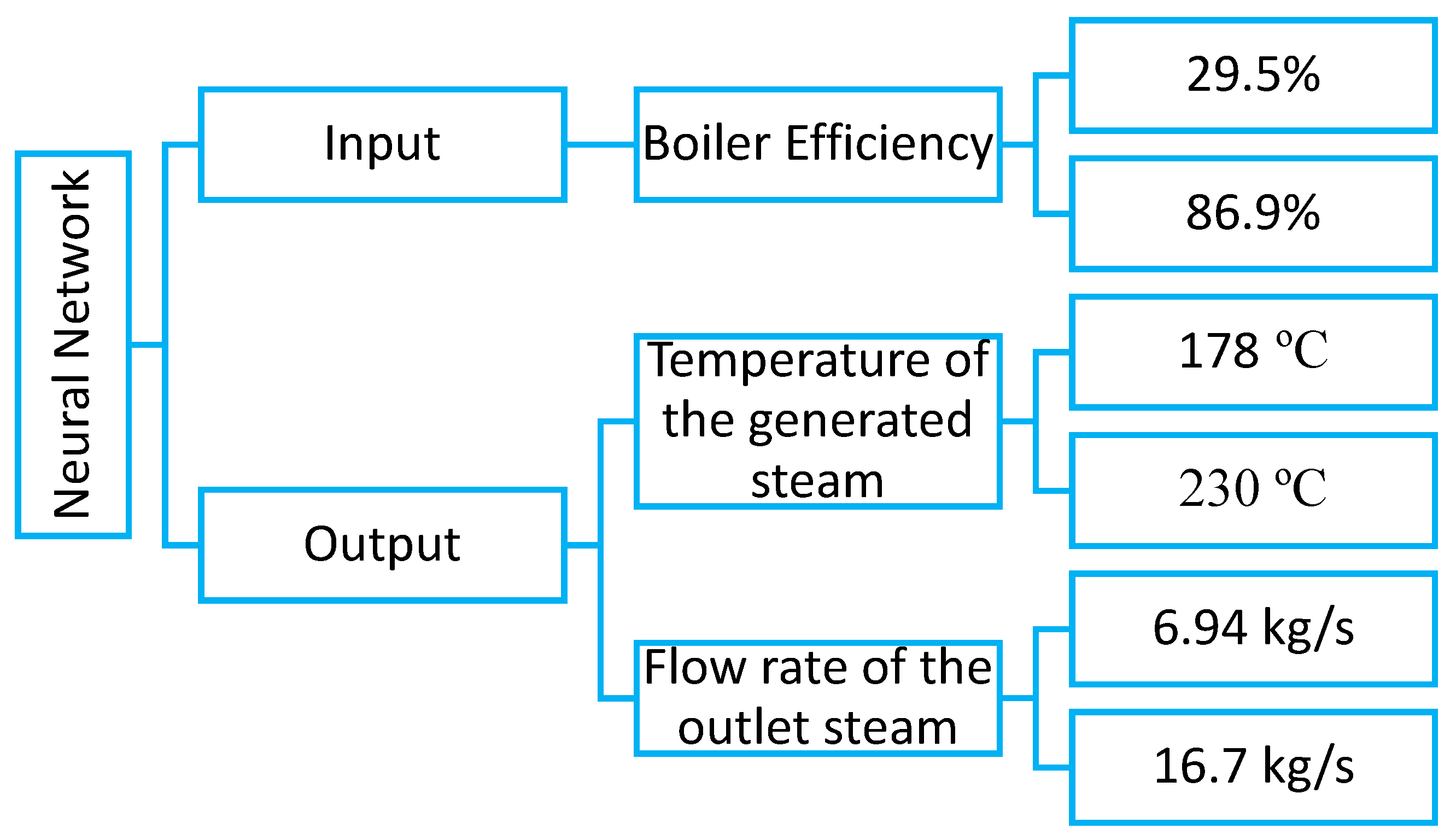
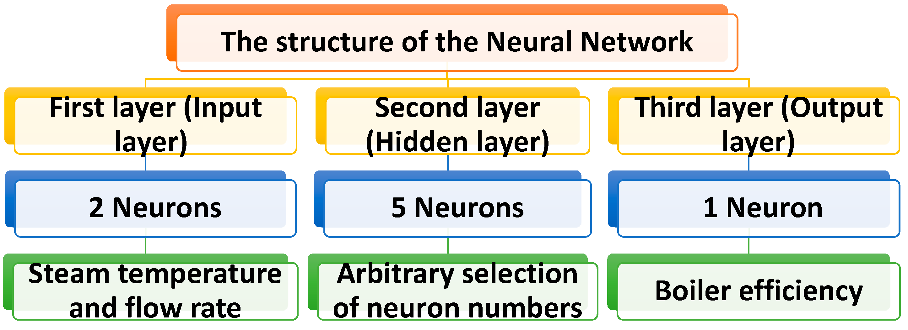
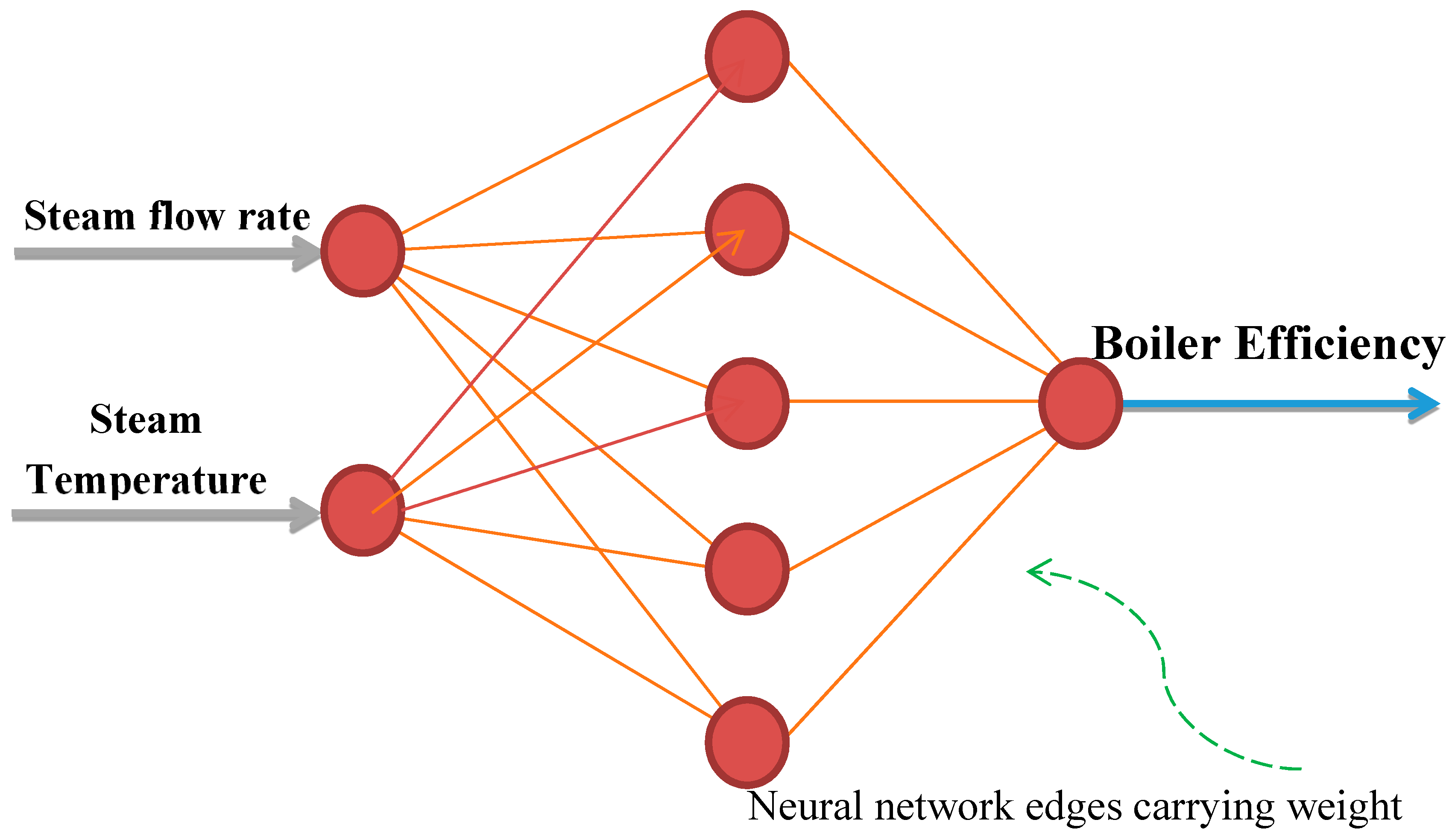
2. Modeling Fundamentals
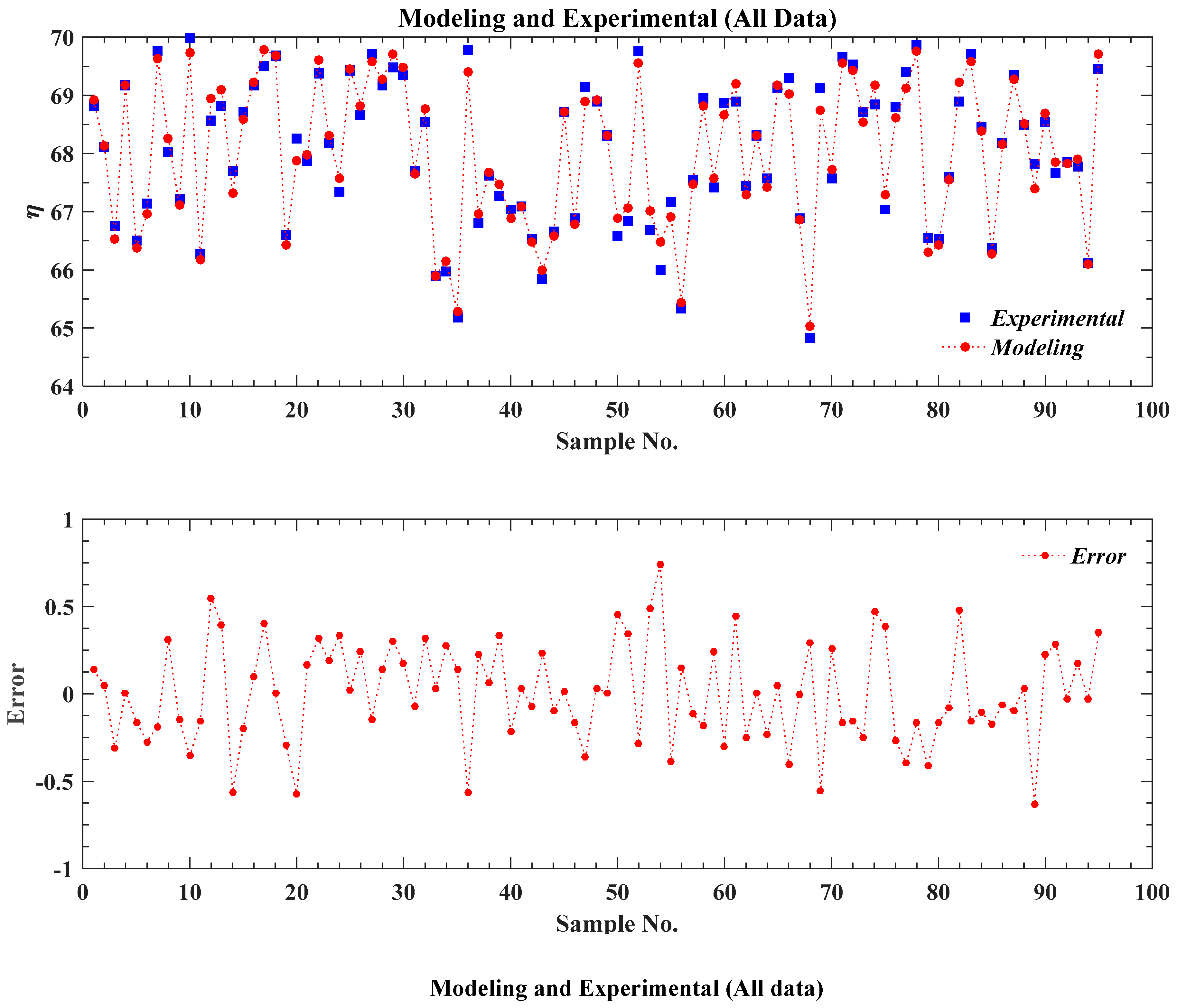
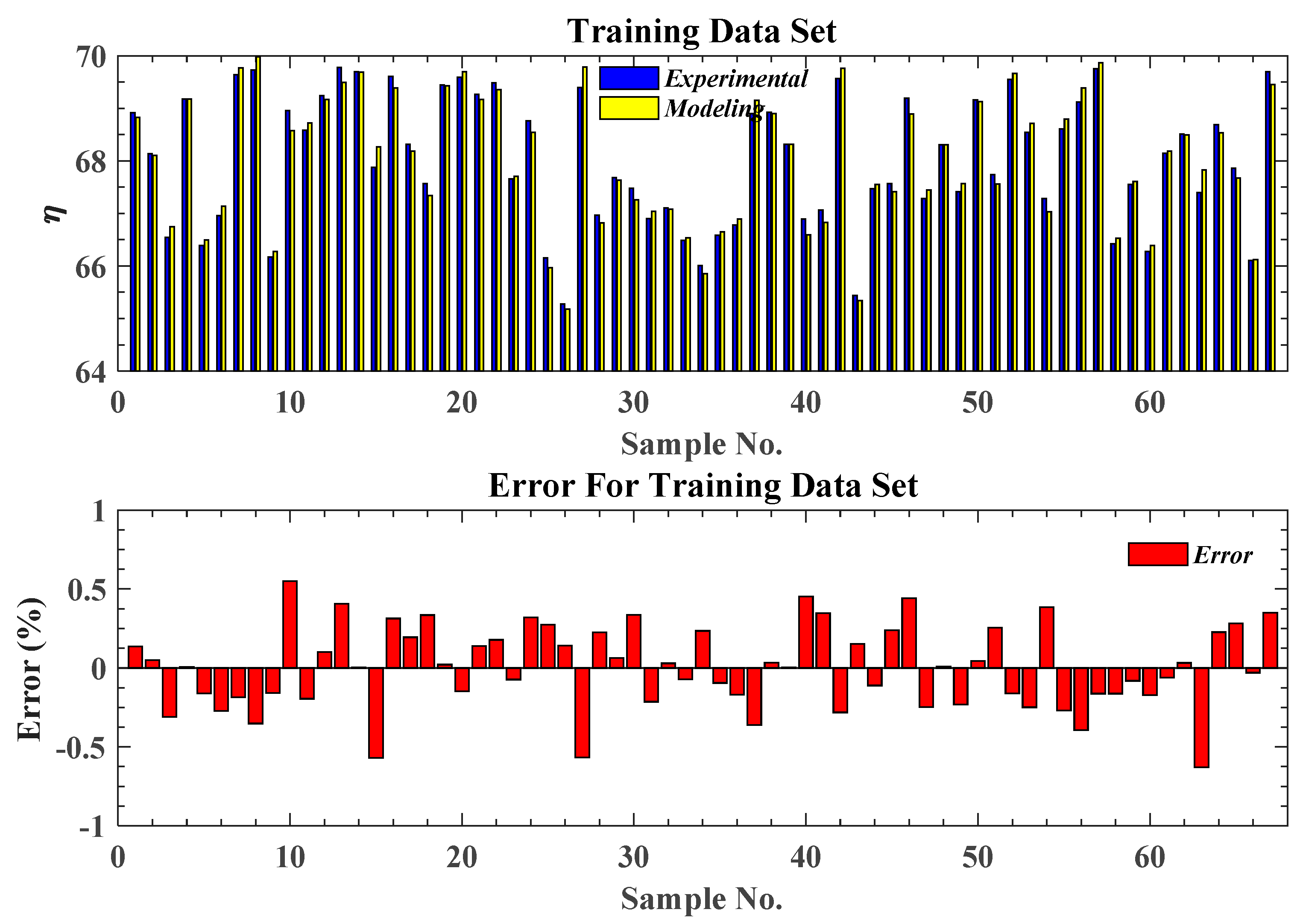
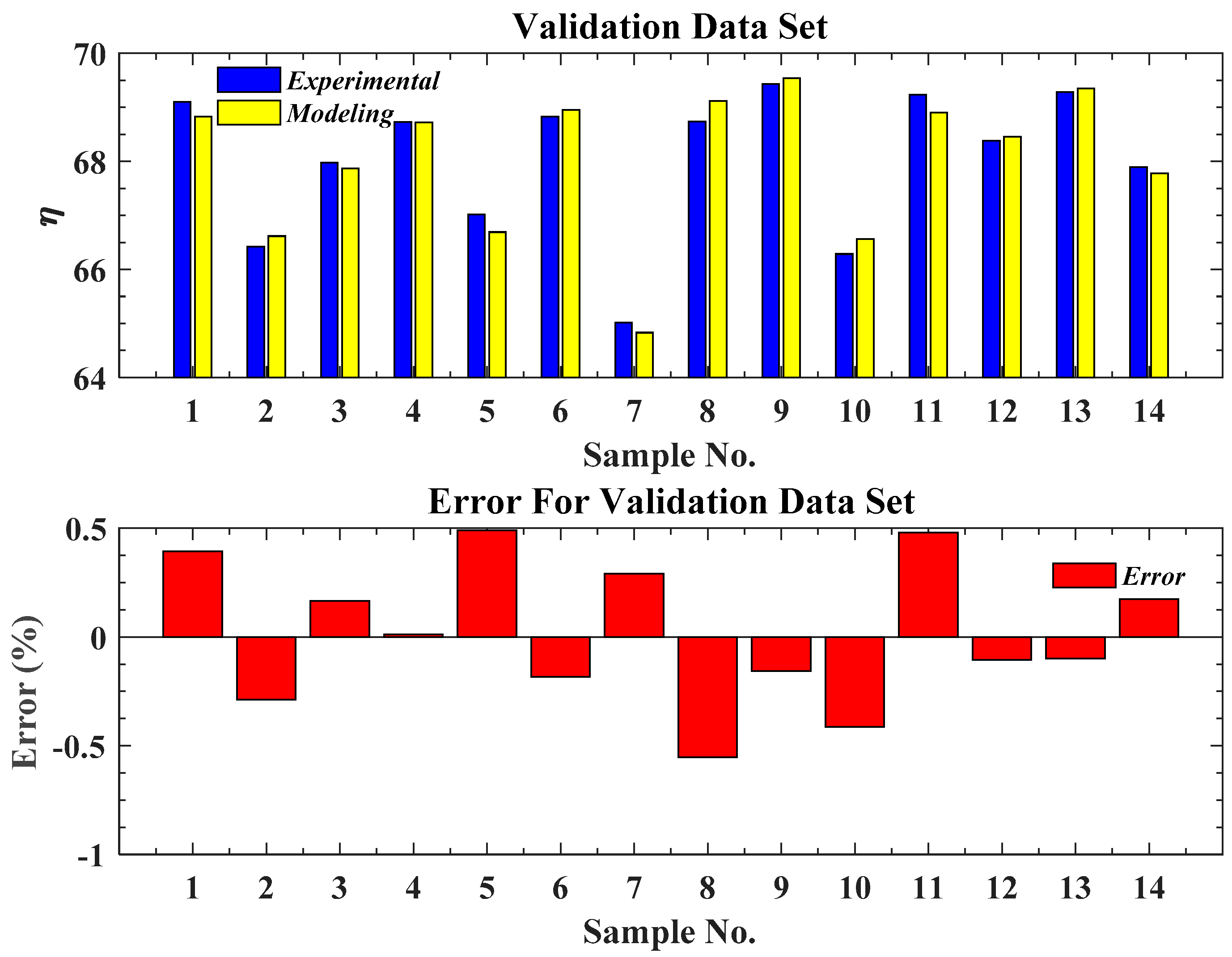
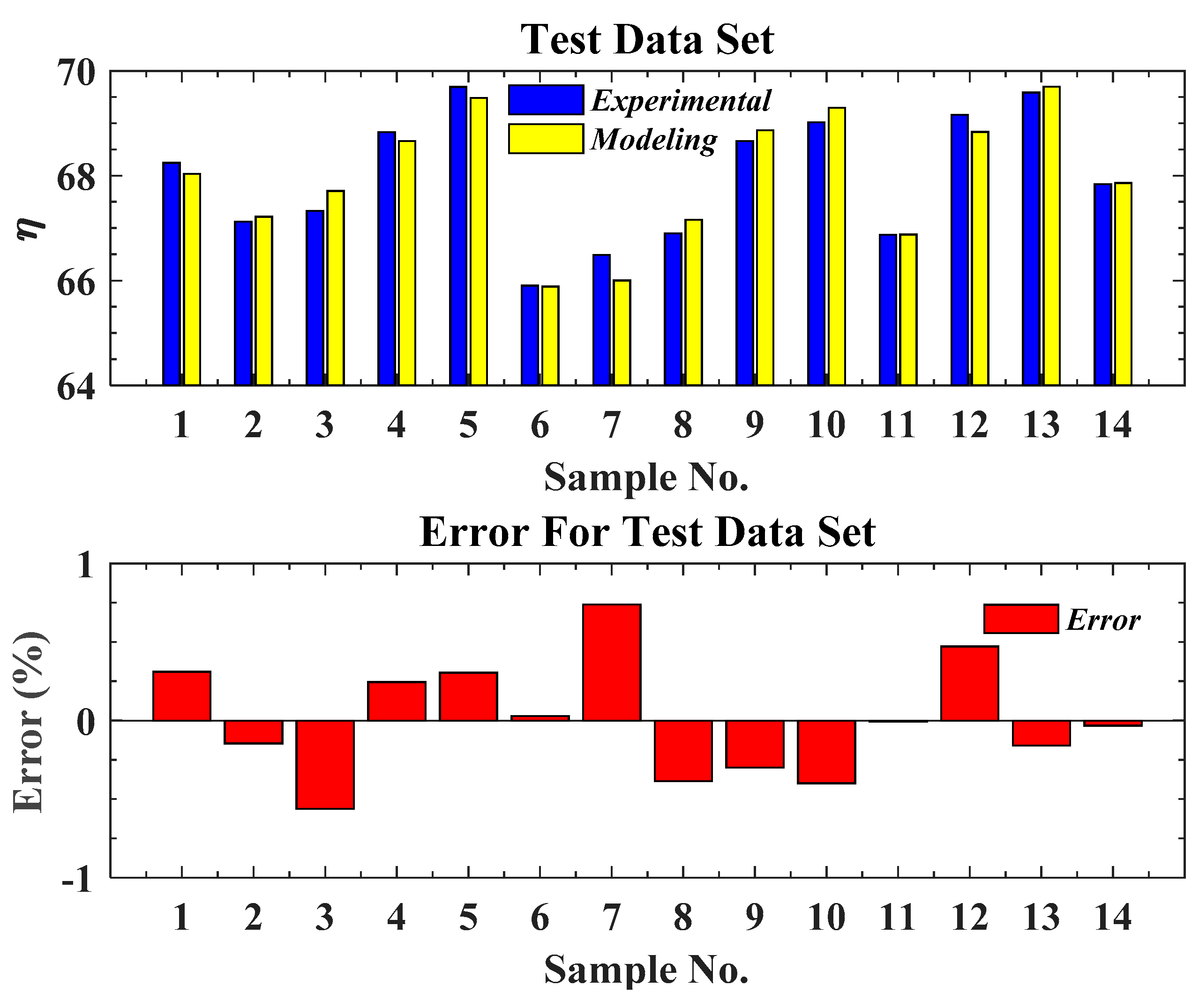
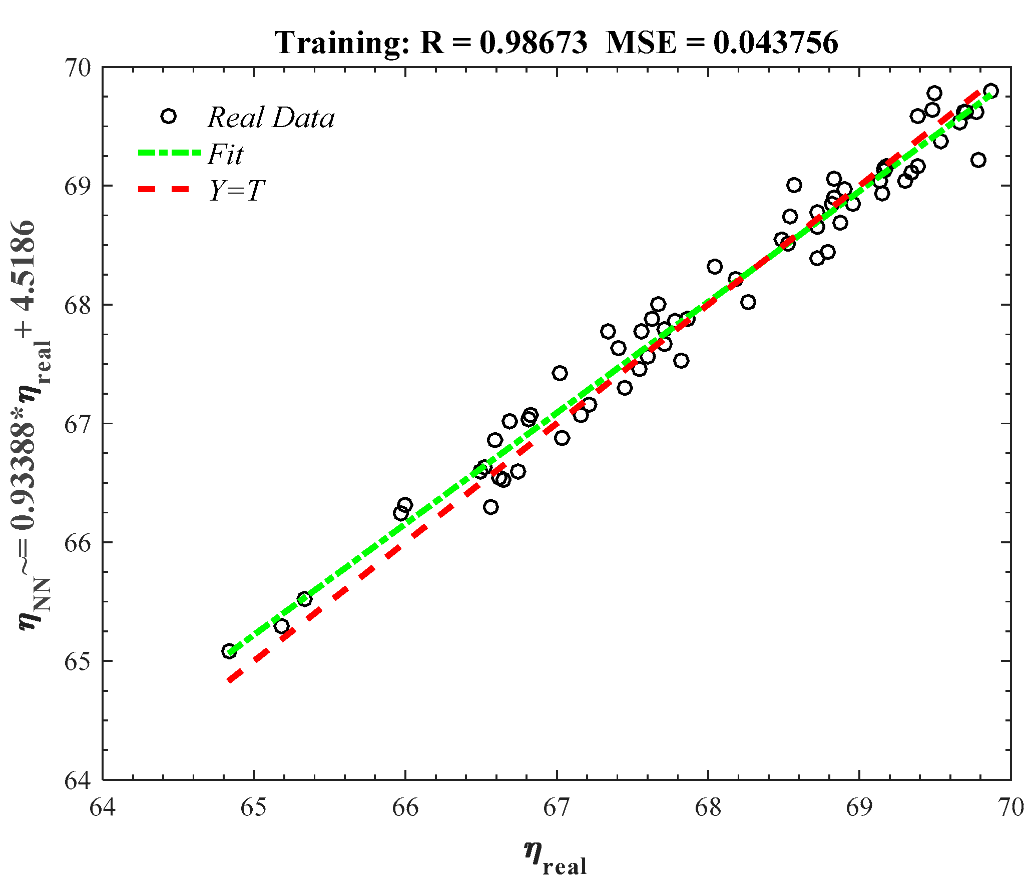
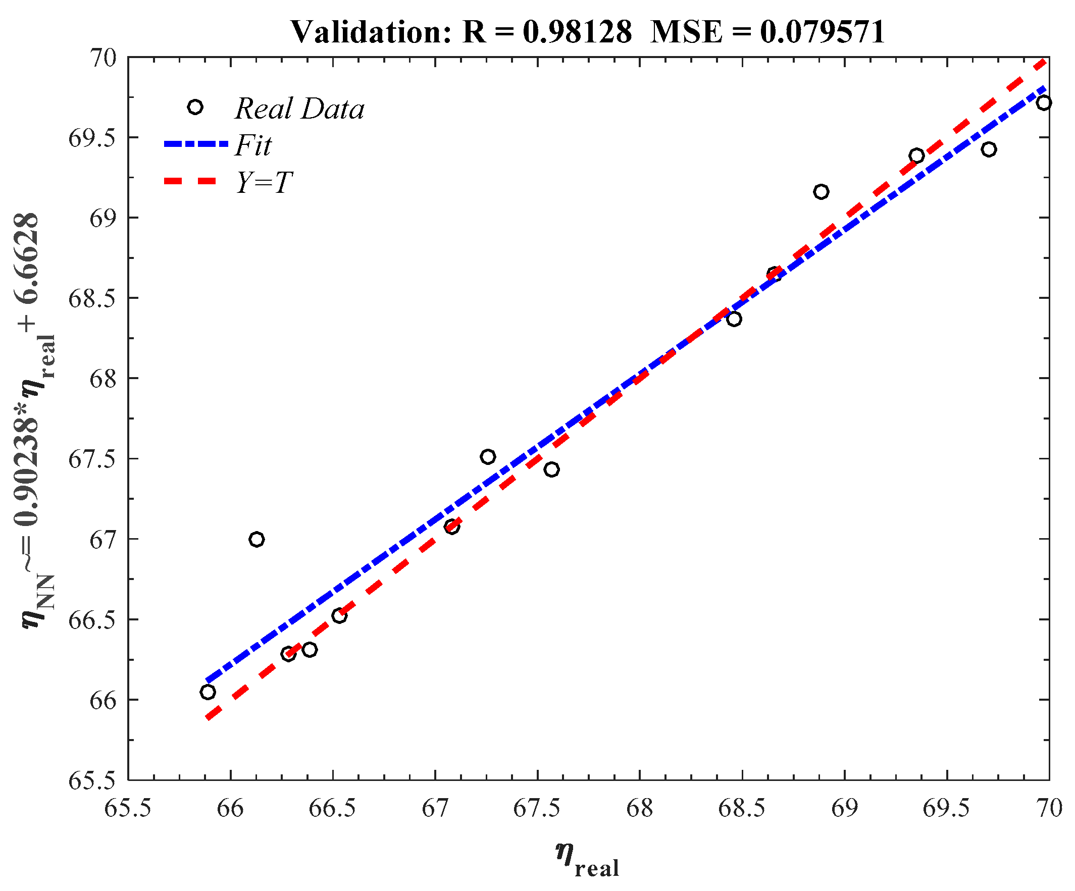
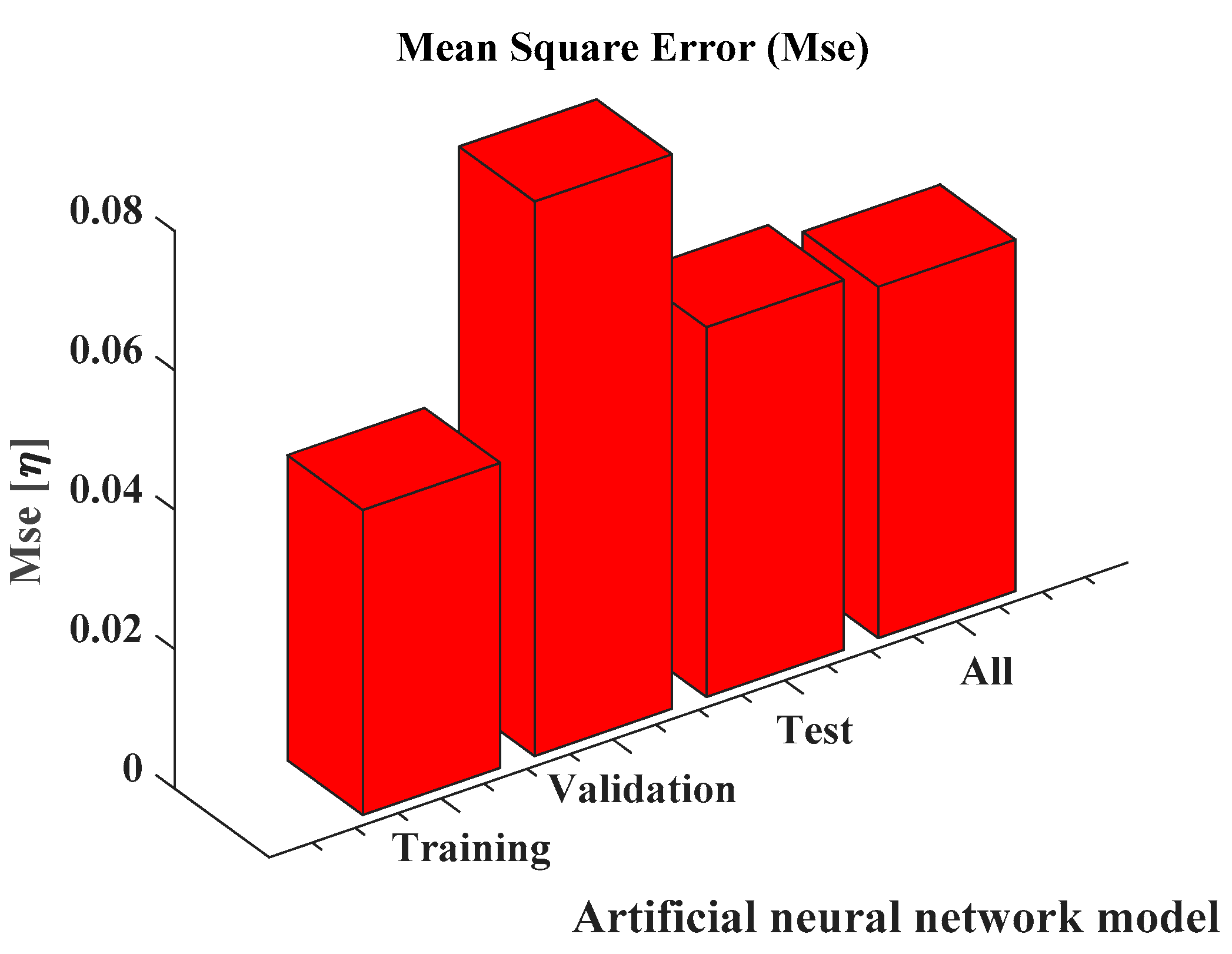
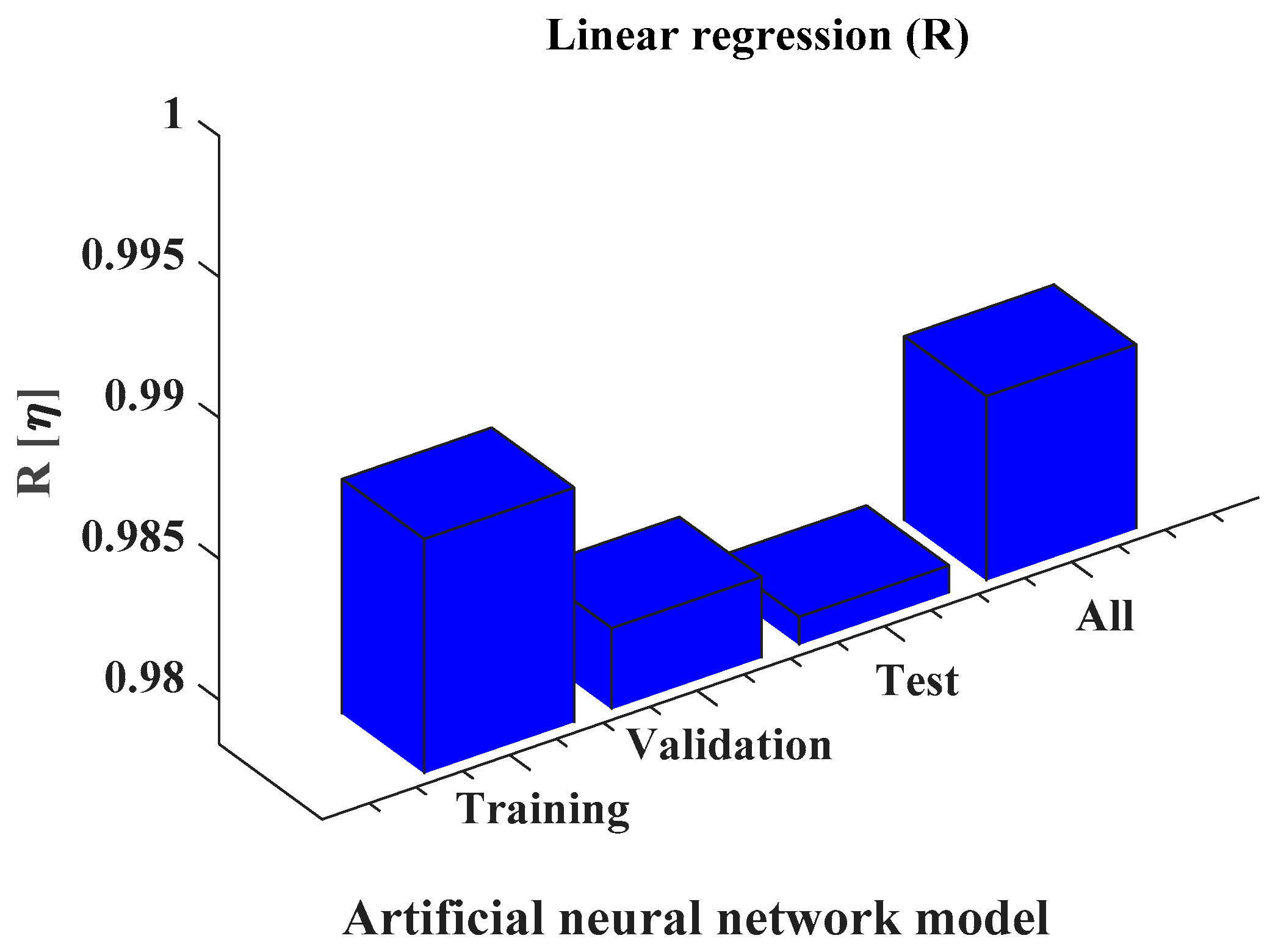
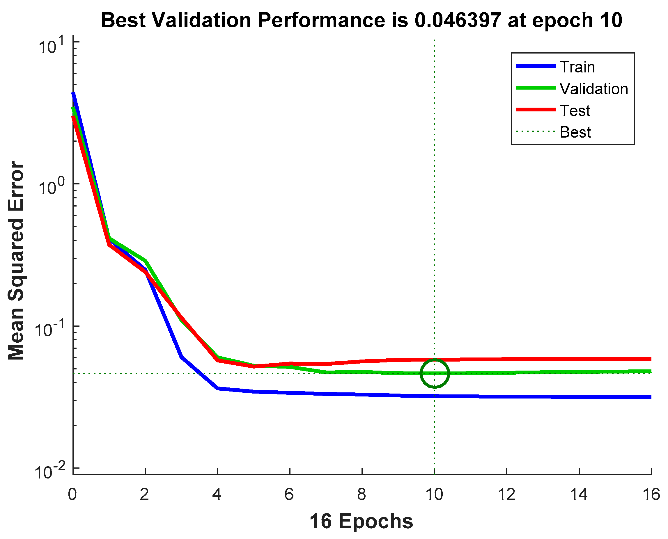
3. Modeling Results of Boiler Efficiency Using Neural Network
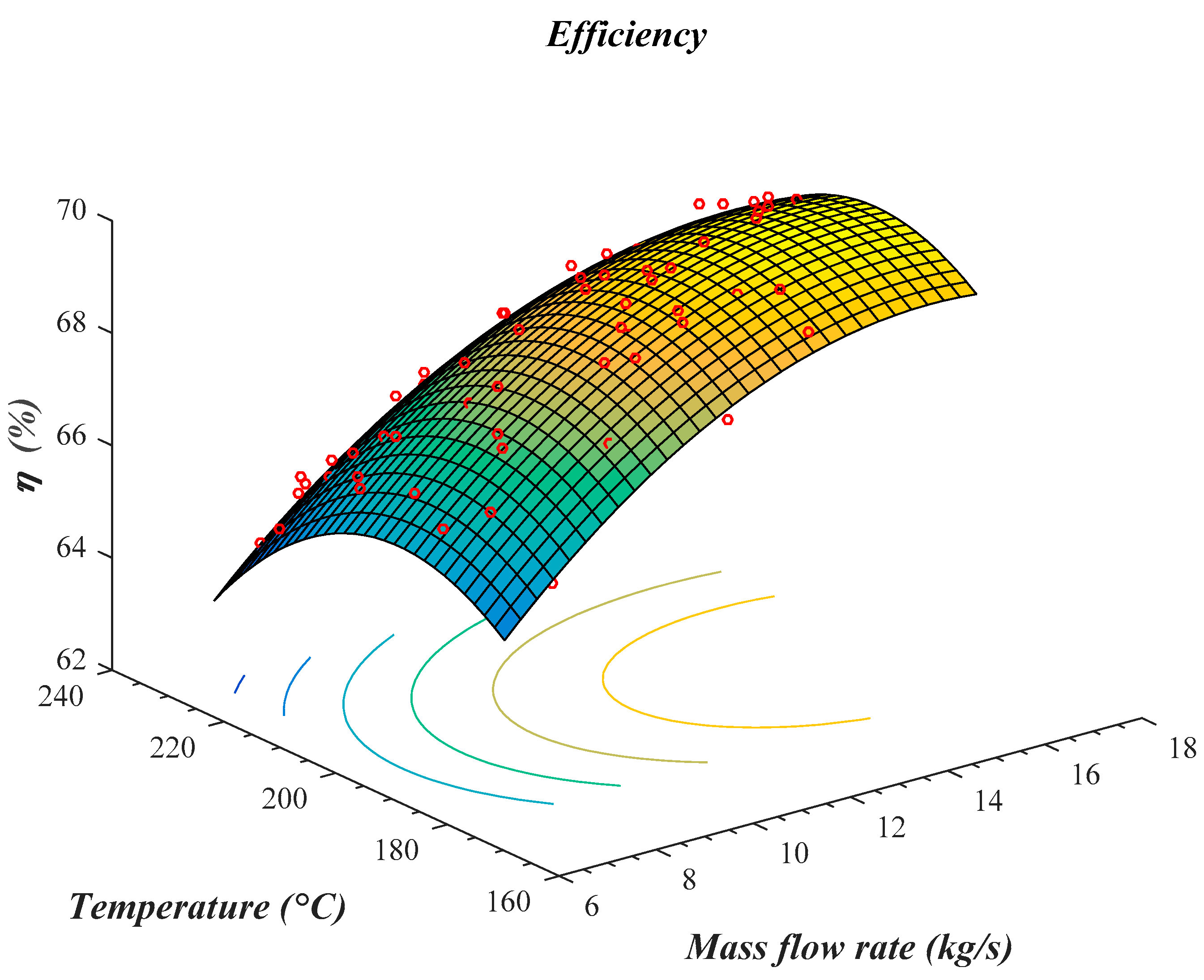
4. Optimization with the Help of the Response-Surface Method
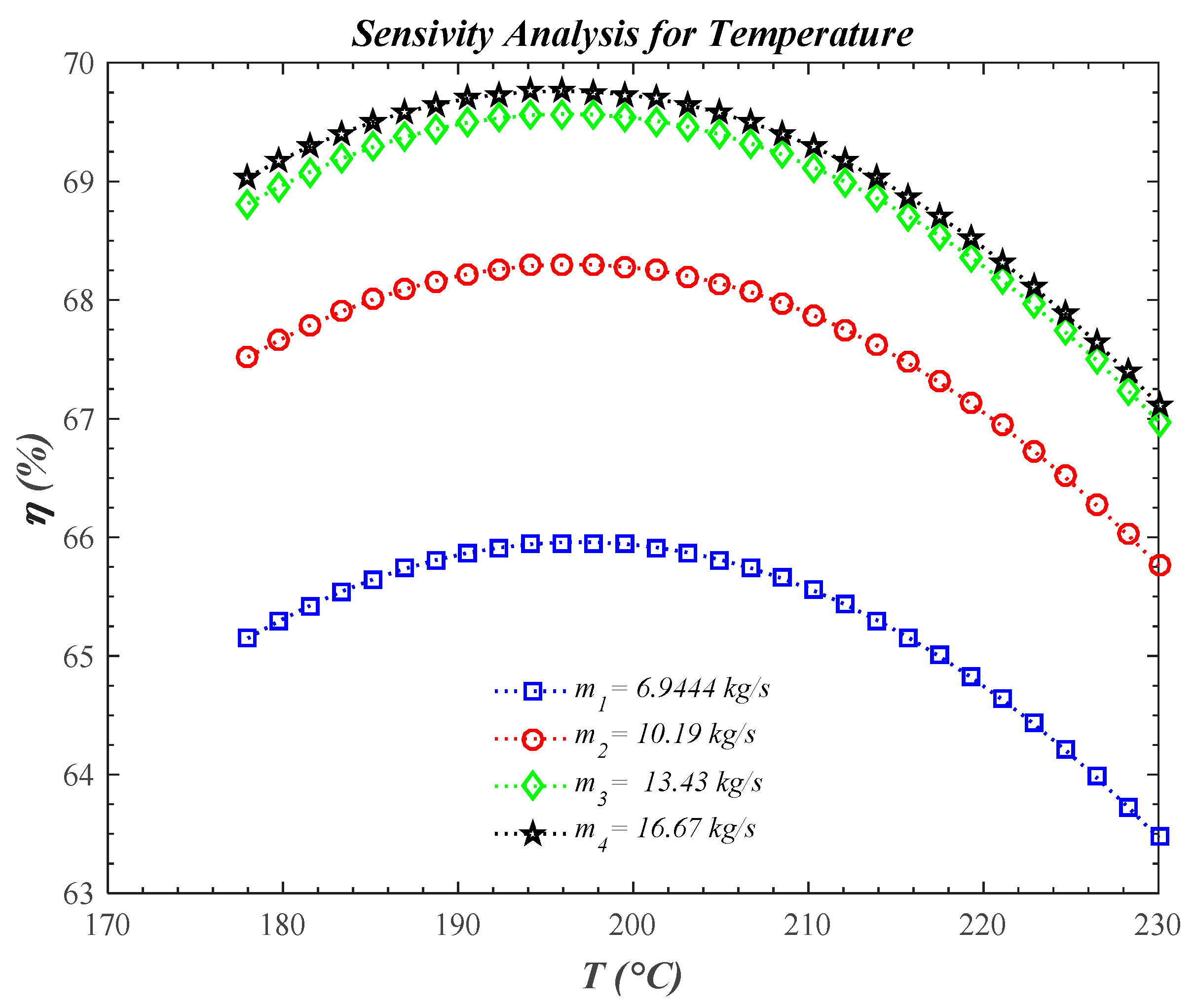
5. Sensitivity Analysis of Effecting Variables
6. Conclusions
Author Contributions
Funding
Conflicts of Interest
References
- Echi, S.; Bouabidi, A.; Driss, Z.; Abid, M.S. CFD simulation and optimization of industrial boiler. Energy 2019, 169, 105–114. [Google Scholar] [CrossRef]
- Ahmadi, M.H.; Alhuyi Nazari, M.; Sadeghzadeh, M.; Pourfayaz, F.; Ghazvini, M.; Ming, T.; Meyer, J.P.; Sharifpur, M. Thermodynamic and economic analysis of performance evaluation of all the thermal power plants: A review. Energy Sci. Eng. 2019, 7, 30–65. [Google Scholar] [CrossRef]
- Szega, M.; Czyż, T. Problems of calculation the energy efficiency of a dual-fuel steam boiler fired with industrial waste gases. Energy 2019, 178, 134–144. [Google Scholar] [CrossRef]
- Mohammadi, A.; Ashouri, M.; Ahmadi, M.H.; Bidi, M.; Sadeghzadeh, M.; Ming, T. Thermoeconomic analysis and multiobjective optimization of a combined gas turbine, steam, and organic Rankine cycle. Energy Sci. Eng. 2018, 6, 506–522. [Google Scholar] [CrossRef] [Green Version]
- Hajebzadeh, H.; Ansari, A.N.M.; Niazi, S. Mathematical modeling and validation of a 320 MW tangentially fired boiler: A case study. Appl. Therm. Eng. 2019, 146, 232–242. [Google Scholar] [CrossRef]
- Shams Ghoreishi, S.M.; Akbari Vakilabadi, M.; Bidi, M.; Khoeini Poorfar, A.; Sadeghzadeh, M.; Ahmadi, M.H.; Ming, T. Analysis, economical and technical enhancement of an organic Rankine cycle recovering waste heat from an exhaust gas stream. Energy Sci. Eng. 2019, 7, 230–254. [Google Scholar] [CrossRef] [Green Version]
- El Hefni, B.; Bouskela, D. Boiler (Steam Generator) Modeling. In Modeling and Simulation of Thermal Power Plants with ThermoSysPro: A Theoretical Introduction and a Practical Guide; Springer International Publishing: Cham, Switzerland, 2019; pp. 153–164. ISBN 978-3-030-05105-1. [Google Scholar]
- Sankar, G.; Kumar, D.S.; Balasubramanian, K.R. Computational modeling of pulverized coal fired boilers —A review on the current position. Fuel 2019, 236, 643–665. [Google Scholar] [CrossRef]
- Trojan, M. Modeling of a steam boiler operation using the boiler nonlinear mathematical model. Energy 2019, 175, 1194–1208. [Google Scholar] [CrossRef]
- Naeimi, A.; Bidi, M.; Ahmadi, M.H.; Kumar, R.; Sadeghzadeh, M.; Alhuyi Nazari, M. Design and exergy analysis of waste heat recovery system and gas engine for power generation in Tehran cement factory. Therm. Sci. Eng. Prog. 2019, 9, 299–307. [Google Scholar] [CrossRef]
- Barroso, J.; Barreras, F.; Amaveda, H.; Lozano, A. On the optimization of boiler efficiency using bagasse as fuel☆. Fuel 2003, 82, 1451–1463. [Google Scholar] [CrossRef]
- Said, S.M.; Hamouda, A.S.; Mahmaoud, H.; Abd-Elwahab, S. Computer-based boiler efficiency improvement. Environ. Prog. Sustain. Energy 2019, 1–9. [Google Scholar] [CrossRef]
- Gungor, K.E.; Winterton, R.H.S. A general correlation for flow boiling in tubes and annuli. Int. J. Heat Mass Transf. 1986, 29, 351–358. [Google Scholar] [CrossRef]
- Kandlikar, S.G. A General Correlation for Saturated Two-Phase Flow Boiling Heat Transfer Inside Horizontal and Vertical Tubes. J. Heat Transf. 1990, 112, 219–228. [Google Scholar] [CrossRef] [Green Version]
- Judd, R.L.; Hwang, K.S. A Comprehensive Model for Nucleate Pool Boiling Heat Transfer Including Microlayer Evaporation. J. Heat Transf. 1976, 98, 623–629. [Google Scholar] [CrossRef]
- Krepper, E.; Rzehak, R. CFD for subcooled flow boiling: Simulation of DEBORA experiments. Nucl. Eng. Des. 2011, 241, 3851–3866. [Google Scholar] [CrossRef]
- Kunkelmann, C.; Stephan, P. CFD simulation of boiling flows using the volume-of-fluid method within OpenFOAM. Numer. Heat Transf. Part A Appl. 2009, 56, 631–646. [Google Scholar] [CrossRef]
- Zhang, X.; Yu, T.; Cong, T.; Peng, M. Effects of interaction models on upward subcooled boiling flow in annulus. Prog. Nucl. Energy 2018, 105, 61–75. [Google Scholar] [CrossRef]
- Promtong, M.; Cheung, S.C.P.; Yeoh, G.H.; Vahaji, S.; Tu, J. CFD investigation of sub-cooled boiling flow using a mechanistic wall heat partitioning approach with Wet-Steam properties. J. Comput. Multiph. Flows 2018, 10, 239–258. [Google Scholar] [CrossRef]
- Pothukuchi, H.; Kelm, S.; Patnaik, B.S.V.; Prasad, B.V.S.S.S.; Allelein, H.-J. Numerical investigation of subcooled flow boiling in an annulus under the influence of eccentricity. Appl. Therm. Eng. 2018, 129, 1604–1617. [Google Scholar] [CrossRef]
- Krepper, E.; Končar, B.; Egorov, Y. CFD modelling of subcooled boiling—Concept, validation and application to fuel assembly design. Nucl. Eng. Des. 2007, 237, 716–731. [Google Scholar] [CrossRef]
- Rivera, W.; Xicale, A. Heat transfer coefficients in two phase flow for the water/lithium bromide mixture used in solar absorption refrigeration systems. Sol. Energy Mater. Sol. Cells 2001, 70, 309–320. [Google Scholar] [CrossRef]
- Owhaib, W.; Palm, B.; Martín-Callizo, C. Flow boiling visualization in a vertical circular minichannel at high vapor quality. Exp. Therm. Fluid Sci. 2006, 30, 755–763. [Google Scholar] [CrossRef]
- Stevanovic, V.; Prica, S.; Maslovaric, B. Multi-Fluid Model Predictions of Gas-Liquid Two-Phase Flows in Vertical Tubes. FME Trans. 2007, 35, 173–181. [Google Scholar]
- Yang, Z.; Peng, X.F.; Ye, P. Numerical and experimental investigation of two phase flow during boiling in a coiled tube. Int. J. Heat Mass Transf. 2008, 51, 1003–1016. [Google Scholar] [CrossRef]
- Kouhikamali, R. Numerical simulation and parametric study of forced convective condensation in cylindrical vertical channels in multiple effect desalination systems. Desalination 2010, 254, 49–57. [Google Scholar] [CrossRef]
- Ozawa, M.; Ami, T.; Umekawa, H.; Matsumoto, R.; Hara, T. Forced flow boiling of carbon dioxide in horizontal mini-channel. Int. J. Therm. Sci. 2011, 50, 296–308. [Google Scholar] [CrossRef]
- Saisorn, S.; Kaew-On, J.; Wongwises, S. An experimental investigation of flow boiling heat transfer of R-134a in horizontal and vertical mini-channels. Exp. Therm. Fluid Sci. 2013, 46, 232–244. [Google Scholar] [CrossRef]
- Shen, Z.; Yang, D.; Chen, G.; Xiao, F. Experimental investigation on heat transfer characteristics of smooth tube with downward flow. Int. J. Heat Mass Transf. 2014, 68, 669–676. [Google Scholar] [CrossRef]
- Chen, L.; Feng, H.; Xie, Z.; Sun, F. Progress of constructal theory in China over the past decade. Int. J. Heat Mass Transf. 2019, 130, 393–419. [Google Scholar] [CrossRef]
- Xie, Z.; Feng, H.; Chen, L.; Wu, Z. Constructal design for supercharged boiler evaporator. Int. J. Heat Mass Transf. 2019, 138, 571–579. [Google Scholar] [CrossRef]
- Behbahaninia, A.; Ramezani, S.; Lotfi Hejrandoost, M. A loss method for exergy auditing of steam boilers. Energy 2017, 140, 253–260. [Google Scholar] [CrossRef]
- Li, C.; Gillum, C.; Toupin, K.; Donaldson, B. Biomass boiler energy conversion system analysis with the aid of exergy-based methods. Energy Convers. Manag. 2015, 103, 665–673. [Google Scholar] [CrossRef]
- Li, Z.; Miao, Z.; Shen, X.; Li, J. Prevention of boiler performance degradation under large primary air ratio scenario in a 660 MW brown coal boiler. Energy 2018, 155, 474–483. [Google Scholar] [CrossRef]
- Li, Z.; Miao, Z.; Zhou, Y.; Wen, S.; Li, J. Influence of increased primary air ratio on boiler performance in a 660 MW brown coal boiler. Energy 2018, 152, 804–817. [Google Scholar] [CrossRef]
- Javan, S.; Ahmadi, P.; Mansoubi, H.; Jaafar, M.N.M. Exergoeconomic Based Optimization of a Gas Fired Steam Power Plant Using Genetic Algorithm. Heat Transf. Res. 2015, 44, 533–551. [Google Scholar] [CrossRef]
- Pattanayak, L.; Ayyagari, S.P.K.; Sahu, J.N. Optimization of sootblowing frequency to improve boiler performance and reduce combustion pollution. Clean Technol. Environ. Policy 2015, 17, 1897–1906. [Google Scholar] [CrossRef]
- Sobota, T. Improving Steam Boiler Operation by On-Line Monitoring of the Strength and Thermal Performance. Heat Transf. Eng. 2018, 39, 1260–1271. [Google Scholar] [CrossRef]
- Nikula, R.-P.; Ruusunen, M.; Leiviskä, K. Data-driven framework for boiler performance monitoring. Appl. Energy 2016, 183, 1374–1388. [Google Scholar] [CrossRef]
- Vandani, A.M.K.; Bidi, M.; Ahmadi, F. Exergy analysis and evolutionary optimization of boiler blowdown heat recovery in steam power plants. Energy Convers. Manag. 2015, 106, 1–9. [Google Scholar] [CrossRef]
- Huang, G.; Huang, G.B.; Song, S.; You, K. Trends in extreme learning machines: A review. Neural Netw. 2015, 61, 32–48. [Google Scholar] [CrossRef]
- Salerno, V.; Rabbeni, G. An Extreme Learning Machine Approach to Effective Energy Disaggregation. Electronics 2018, 7, 235. [Google Scholar] [CrossRef]
- Hussain, T.; Siniscalchi, S.M.; Lee, C.C.; Wang, S.S.; Tsao, Y.; Liao, W.H. Experimental study on extreme learning machine applications for speech enhancement. IEEE Access 2017, 5, 25542–25554. [Google Scholar] [CrossRef]
- Hinton, G.E. Training Products of Experts by Minimizing Contrastive Divergence. Neural Comput. 2002, 14, 1771–1800. [Google Scholar] [CrossRef] [PubMed]
- Sadeghzadeh, M.; Ahmadi, M.H.; Kahani, M.; Sakhaeinia, H.; Chaji, H.; Chen, L. Smart modeling by using artificial intelligent techniques on thermal performance of flat-plate solar collector using nanofluid. Energy Sci. Eng. 2019, 1–10. [Google Scholar] [CrossRef]
- Kahani, M.; Ahmadi, M.H.; Tatar, A.; Sadeghzadeh, M. Development of multilayer perceptron artificial neural network (MLP-ANN) and least square support vector machine (LSSVM) models to predict Nusselt number and pressure drop of TiO2/water nanofluid flows through non-straight pathways. Numer. Heat Transf. Part A Appl. 2018, 74, 1190–1206. [Google Scholar] [CrossRef]


| η | η | ||||
|---|---|---|---|---|---|
| 5.06277 | 179.8114 | 68.8229 | 10.3826 | 202.5607 | 68.3157 |
| 11.50799 | 217.4076 | 68.10162 | 8.112843 | 195.3354 | 66.59289 |
| 10.96721 | 227.7698 | 66.7485 | 12.47747 | 228.7439 | 66.83186 |
| 11.83226 | 195.8293 | 69.17249 | 15.45171 | 206.8831 | 69.76082 |
| 8.164 | 211.1887 | 66.49393 | 10.33337 | 222.0078 | 66.69333 |
| 8.230552 | 195.8363 | 67.13933 | 7.35201 | 199.2193 | 66.00094 |
| 15.4074 | 189.2565 | 69.76787 | 8.328303 | 202.0249 | 67.16067 |
| 12.80646 | 218.8824 | 68.03788 | 7.689097 | 220.9679 | 65.33974 |
| 9.523767 | 215.6007 | 67.21874 | 14.14401 | 229.5426 | 67.54719 |
| 15.35225 | 192.4996 | 69.97655 | 11.38288 | 205.2453 | 68.95443 |
| 7.509398 | 208.2864 | 66.27828 | 13.44131 | 226.1227 | 67.40915 |
| 11.39483 | 199.8923 | 68.57542 | 13.74267 | 216.4291 | 68.86722 |
| 13.96593 | 182.7876 | 68.82806 | 12.49931 | 207.5064 | 68.88944 |
| 10.24027 | 179.2494 | 67.70906 | 13.05674 | 228.3764 | 67.44843 |
| 10.84519 | 203.5396 | 68.7183 | 15.47826 | 220.874 | 68.30319 |
| 12.06786 | 192.4699 | 69.16695 | 13.38398 | 227.8997 | 67.56851 |
| 15.6384 | 195.6674 | 69.49326 | 15.45541 | 211.61 | 69.13087 |
| 14.51184 | 192.9422 | 69.69088 | 11.48975 | 197.7378 | 69.29713 |
| 7.618852 | 186.887 | 66.61787 | 8.318545 | 202.7819 | 66.87618 |
| 9.65485 | 198.7617 | 68.26366 | 7.606863 | 225.4183 | 64.83067 |
| 10.63276 | 214.2778 | 67.86751 | 13.88847 | 178.7724 | 69.11839 |
| 15.35098 | 188.5912 | 69.38854 | 9.938753 | 186.1481 | 67.56152 |
| 11.02739 | 212.649 | 68.18121 | 13.46965 | 202.5215 | 69.66543 |
| 9.276587 | 201.0394 | 67.34079 | 13.28742 | 206.2356 | 69.53684 |
| 12.75497 | 200.5314 | 69.42711 | 12.10742 | 181.1039 | 68.71523 |
| 11.60532 | 187.1125 | 68.66235 | 13.89687 | 212.2176 | 68.83852 |
| 15.68032 | 188.0465 | 69.69601 | 11.85233 | 224.261 | 67.02746 |
| 16.0319 | 210.0539 | 69.16832 | 11.68888 | 183.7009 | 68.7909 |
| 14.89612 | 191.9886 | 69.48701 | 11.78454 | 200.7642 | 69.38998 |
| 13.83662 | 207.1033 | 69.35699 | 16.04421 | 192.572 | 69.86828 |
| 14.1702 | 227.1288 | 67.70859 | 10.72913 | 229.2328 | 66.56324 |
| 15.69162 | 215.1525 | 68.53946 | 8.083356 | 209.6555 | 66.52948 |
| 7.57872 | 213.3194 | 65.88433 | 9.281896 | 191.195 | 67.60546 |
| 10.21025 | 227.8878 | 65.96942 | 13.60328 | 184.896 | 68.9027 |
| 6.986591 | 218.3174 | 65.18013 | 15.10385 | 206.3403 | 69.70184 |
| 14.99537 | 209.6018 | 69.78638 | 16.37641 | 221.0458 | 68.45829 |
| 11.87784 | 227.2961 | 66.81758 | 9.036371 | 221.5243 | 66.38769 |
| 10.50436 | 181.1014 | 67.63481 | 14.33667 | 221.3341 | 68.1886 |
| 9.147886 | 191.973 | 67.25517 | 12.62322 | 188.5932 | 69.35013 |
| 12.1442 | 229.3074 | 67.04037 | 10.86203 | 206.3097 | 68.49007 |
| 9.758881 | 218.1548 | 67.08144 | 11.90317 | 223.497 | 67.82707 |
| 7.609162 | 202.7184 | 66.5345 | 11.76321 | 184.292 | 68.53394 |
| 7.770549 | 213.4068 | 65.85192 | 13.27719 | 222.5302 | 67.67154 |
| 7.608856 | 199.6806 | 66.64859 | 14.17492 | 224.7884 | 67.86074 |
| 10.92877 | 197.7678 | 68.71765 | 9.880103 | 189.329 | 67.77672 |
| 8.143986 | 189.0901 | 66.894 | 7.815672 | 182.0029 | 66.12302 |
| 11.25155 | 197.9128 | 69.15146 | 14.97466 | 202.6592 | 69.45441 |
| 15.68414 | 179.5427 | 68.899 |
| Variable | Definition | Description |
|---|---|---|
| Output of the neural network model | Boiler efficiency, the final output of the neural network model | |
| 1st input variable | Steam mass flow rate, kg/s | |
| 2nd input variable | Temperature, | |
| Edge matrix between 1st and 2nd layers | Each of the edges between layer 1 and 2 is assigned a weight | |
| Edge matrix between 2nd and 3rd layers | Each of the edges between layer 2 and 3 is assigned a weight | |
| Bias matrix of the 2nd layer | After multiplying the weight matrix in the input signal, the results are summed with the bias. | |
| Bias matrix of the 3rd layer | After multiplying the weight matrix in the input signal, the results are summed with the bias. |
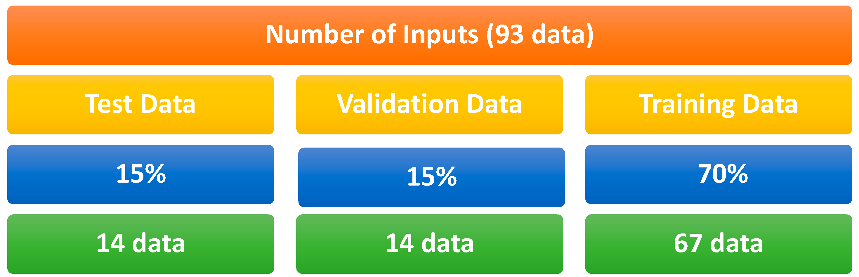
| Train (70%) | Validation (15%) | Test (15%) | |
|---|---|---|---|
| Number of data | 67 | 14 | 14 |
| Mean squared error (MSE) | 0.043 | 0.079 | 0.053 |
| Regression coefficient (R2) | 0.986 | 0.981 | 0.979 |
| Constants | C0 | C1 | C2 | C12 | C11 | C22 |
|---|---|---|---|---|---|---|
| Optimized Value | −31.372 | 1.690 | 0.8977 | −0.00047 | −0.05112 | −0.00227 |
| Variable | Objective Function | 1st Independent Variable | 2nd Independent Variable |
|---|---|---|---|
| Unit | Efficiency (%) | Flow rate (kg/s) | Temperature () |
| Optimal value from RSM | 69.8 | 15.7 | 195.9 |
© 2019 by the authors. Licensee MDPI, Basel, Switzerland. This article is an open access article distributed under the terms and conditions of the Creative Commons Attribution (CC BY) license (http://creativecommons.org/licenses/by/4.0/).
Share and Cite
Maddah, H.; Sadeghzadeh, M.; Ahmadi, M.H.; Kumar, R.; Shamshirband, S. Modeling and Efficiency Optimization of Steam Boilers by Employing Neural Networks and Response-Surface Method (RSM). Mathematics 2019, 7, 629. https://0-doi-org.brum.beds.ac.uk/10.3390/math7070629
Maddah H, Sadeghzadeh M, Ahmadi MH, Kumar R, Shamshirband S. Modeling and Efficiency Optimization of Steam Boilers by Employing Neural Networks and Response-Surface Method (RSM). Mathematics. 2019; 7(7):629. https://0-doi-org.brum.beds.ac.uk/10.3390/math7070629
Chicago/Turabian StyleMaddah, Heydar, Milad Sadeghzadeh, Mohammad Hossein Ahmadi, Ravinder Kumar, and Shahaboddin Shamshirband. 2019. "Modeling and Efficiency Optimization of Steam Boilers by Employing Neural Networks and Response-Surface Method (RSM)" Mathematics 7, no. 7: 629. https://0-doi-org.brum.beds.ac.uk/10.3390/math7070629