Dynamic Properties of Foreign Exchange Complex Network

Abstract

The foreign exchange (FX) market, one of the important components of the financial market, is a typical complex system. In this paper, by resorting to the complex network method, we use the daily closing prices of 41 FX markets to build the dynamical networks and their minimum spanning tree (MST) maps by virtue of a moving window correlation coefficient. The properties of FX networks are characterized by the normalized tree length, node degree distributions, centrality measures and edge survival ratios. Empirical results show that: (i) the normalized tree length plays a role in identifying crises and is negatively correlated with the market return and volatility; (ii) 83% of FX networks follow power-law node degree distribution, which means that the FX market is a typical heterogeneous market, and a few hub nodes play key roles in the market; (iii) the highest centrality measures reveal that the USD, EUR and CNY are the three most powerful currencies in FX markets; and (iv) the edge survival ratio analysis implies that the FX structure is relatively stable.

1. Introduction

The foreign exchange (FX) market is the most liquid and largest financial market [1,2,3]. It identifies the exchange rates of global trade and also determines the relative wealth of a country [4,5,6]. The volatility of the FX market is affected by many factors, and its occurrence, formation and evolution show the typical feature of complex system [7,8,9]. To date, networks and dynamics modeling have attracted great attention in natural, social science and engineering technology [10,11,12,13,14,15,16,17,18,19,20,21,22]. Using complex network theory to study the FX market has become popular [23,24,25,26,27,28,29].

In general, there are two methods to build FX networks: one is to use static methods and the other is to employ time-varying methods. Mcdonald et al. [30] was the pioneer for adopting the Pearson correlation coefficient and the minimum spanning tree (MST) method to build the static FX network and found that USD was predominant. Thereafter, similar studies applied these methods to analyze the static FX network topology, such as community structure [31,32,33], node degree distributions [34] and centrality measures [35,36,37]. In addition, other methods are adopted to establish an FX network and studied their static characteristics. Wang and Xie [38] applied the copula model and the MST method to build an FX network, and the study found that USD plays a dominant role in the FX market. Cao et al. [39] utilized the mutual information method and threshold method to set up an FX network, and the research found that the FX network displayed small world properties.

Notably, the literature above is all based on topology properties of the static FX network. However, the FX market is constantly changing and the connections between the FX network are variable. Dynamic FX networks are better to describe the structural variation. Fenn et al. [40] used the moving window Pearson correlation coefficient and the MST method to construct dynamic FX networks and found that community structure had a significant change during the sub-prime crisis. Similarly, Wang et al. [41] found that USD was the most influential currency during the sub-prime crisis. Fenn et al. [42] discovered that the communities of the FX network had an obvious variation during the Mexican peso crisis, the Asian currency crisis and the sub-prime crisis.

The studies of dynamic FX networks are related to the structural variation during the significant events, such as the Mexican peso crisis, the Asian currency crisis and the sub-prime crisis [40,41,42]. Some research has also confirmed that the European debt crisis and the CNY’s participation in special drawing rights has an impact on the FX market [43,44]. However, these studies lack a network perspective because of FX markets being interconnected [45]. In addition, investors are more concerned about the return [46,47,48,49,50] and volatility [51,52,53,54,55] levels of the FX market. Literature dealing with the relationship between the topology variation of networks and FX market’s return and volatility has not been studied. Such research not only helps us understand the topology variation of FX networks, but also provides good guidance for the risk management of FX investment.

In this paper, we employ a moving window Pearson correlation coefficient in the daily closing prices of 41 FX markets from January 2005 to December 2017. Then, we use the MST method to construct the corresponding networks. The topology evolution of FX networks is depicted by the normalized tree length, node degree distributions, centrality measures and edge survival ratios.

The crucial novelty of this paper is highlighted in the following aspects:

• Taking fully into consideration of the temporal characteristics of the FX market, using the method of the moving window correlation coefficient, we establish dynamic networks instead of a static network to investigate the FX market.
• This paper originally revealed that the normalized tree length of the FX network is strongly correlated with the European debt crisis and the CNY’s participation in special drawing rights by employing the complex network method.
• Literature dealing with the FX market is largely restricted to the return and volatility; investigation combining the topology variation of FX networks and market’s return and volatility appears to be scarce. Our research fills this gap.

The reminder of this paper is arranged as follows: Section 2 introduces the methodology. Section 3 gives an empirical analysis. Section 4 presents some conclusions.

2. Methodology

In this section, we first propose a moving window correlation coefficient and the MST method to construct dynamic FX networks. Then, in order to measure the properties of networks, we introduce the definitions of normalized tree length, node degree distribution, node degree and node strength, betweenness centrality, closeness centrality and edge survival ratio. Lastly, we present measures of market phenomena, such as the moving window return and volatility.

2.1. Network Construction

A network is generally defined as a set of nodes linked by edges. If we build time-varying FX networks, each FX market represents a network node, and each pair of the FX markets is linked with an edge calculated by a moving window Pearson correlation coefficient. Although the Pearson correlation coefficient neglects the analysis of monotonic associations [56], it is the simplest method to describe the correlation between financial market and is widely used to construct FX network [30,31,32,33].

The evolution process of the FX network is investigated by setting a time window with a length of T days and moving the window along time. A new network is gained after each window replacement. This procedure is repeated until the end of the original time series is attained. In other words, the first network is established by using Pearson correlation coefficient to calculate the correlation between each pair of FX returns from the sample beginning at day $t_1^1=1$ and terminating at day $t_2^1=\phi$. The Pearson correlation coefficient of the return series of FX i and j in the mth window is defined as:

$$C_{i,j}^m=\frac{〈R_i^m{R}_j^m〉-〈R_i^m〉〈R_j^m〉}{\sqrt{\left.\left({\left.〈R_i^m\right)}^2\right.〉-{〈R_i^m〉}^2\right)\left(〈{\left(R_j^m\right)}^2〉-{〈R_j^m〉}^2\right)}},$$

(1)

where $\langle \cdots \rangle$ represent the statistical mean value, $-1\le C_{i,j}^m\le 1$, $R_i^m\left(t\right)=lnC{P}_i^m\left(t\right)-lnC{P}_i^m(t-1)$, $R_i^m\left(t\right)$ stands for FX i at day t in the mth window and $C{P}_i^m\left(t\right)$ denotes the closing price of FX rates i on days t.

The second network is built by employing Pearson correlation coefficient to calculate the correlation between each pair of FX returns from the sample starting at day $t_1^2=1+\tau$ and ending at day $t_2^2=\phi +\tau$, and so on. Consequently, we can get the number of N ($N=1+T-\phi$) networks.

However, such Pearson correlation coefficient network displays all the connections, which could cause the picture to be unreadable [36]. Minimum spanning tree (MST) graph is an appropriate method in this paper [30,31,32,33].

Before we obtain a MST network, the Pearson correlation coefficient matrix ought to be converted into a distance matrix according to Mantegna [57]. The distances are defined as follows:

$$d_{i,j}^m=\sqrt{2\left(1-C_{i,j}^m\right)}.$$

(2)

Based on the obtained distance matrix, this paper adopts the MST method to construct the FX network according to the Kruskal [58] algorithm. Here is a brief introduction to the MST method:

(1)

Created a network edge matrix (which contains $\left(41\times 41\right)/\phantom{\left(41\times 41\right)2}2$ edges) and sorted increase progressively based on distances.

(2)

Chose the first element (that is, the smallest distance) and connected them to form one edge.

(3)

Selected the next element and connected to constitute an edge. If it can make the network graph tree-like (ie, it cannot form a ring), then the edge was kept, otherwise the edge was abandoned.

(4)

Repeated step (3) until all elements were exhausted.

We construct the MST network in each window, and one thus obtains N successive networks.

2.2. Network Topological Properties

2.2.1. Normalized Tree Length

Normalized tree length (NTL) captures the FX network’s average distance of edges [59]. It is defined as:

$$\begin{array}{c}\hfill NT{L}^m=\frac{1}{N-1}\sum _{d_{a,b}^m\in E^m}{d}_{a,b}^m,\end{array}$$

(3)

where $d_{a,b}^m$ stands for the distance from node a to node b, and $E^m$ denotes the edge set of the FX network.

2.2.2. Node Degree and Node Strength

Node degree denotes the quantity of nodes which is adjacent to node i [60]. It is defined as:

$$\begin{array}{c}\hfill k_i=\sum _{j\in N_i}{A}_{ij},\end{array}$$

(4)

where $A_{ij}$ represents the adjacent matrix to the FX network.

Node strength reflects the importance of the node’s on FX network. It is defined as [61]:

$$\begin{array}{c}\hfill s_i=\sum _{j\in N_i}{w}_{ij},\end{array}$$

(5)

where $N_i$ is the number of neighbor node; $w_{ij}$ represents the Pearson correlation coefficient between node i and node j.

2.2.3. Node Degree Distribution

A large number of studies have been demonstrated that the node degree of numerous actual networks obey paw-law distribution [62,63,64]. The cumulative distribution function of node degree is defined as:

$$\begin{array}{c}\hfill P\left(k\right)={\left(\frac{k}{k_{min}}\right)}^{-\beta +1},\end{array}$$

(6)

where k is expressed as the degree set of the node $\left\{k_i\left|i=1,2,\cdots ,N\right.\right\}$, $k_{min}$ represents the power-law’s lower bound model, and the $\beta$ can be estimated by maximum likelihood.

Generally, in order to judge for the power-law distribution, there are several statistics, such as Cramer–von Mises, Kolmogorov–Smirnov, Anderson–Darling, Kuiper V, Watson U2, and H1 Statistic are employed [65]. This paper employs the K–S statistic to judge for it because the K–S statistic is one of the commonly adopted statistics to identify whether the degree of nodes obeys power-law distribution [66,67,68].

2.2.4. Betweenness Centrality

The betweenness centrality ($C_B\left(v_c\right)$ ) describes the intermediate process between other nodes. The larger value of $C_B\left(v_c\right)$, the more important positions a node possesses [69]. It is defined as:

$$\begin{array}{c}\hfill C_B\left(v_c\right)=\frac{1}{\left(N-2\right)\left(N-1\right)}\sum _{a,b}\frac{n_{ab}\left(c\right)}{n_{ab}},\end{array}$$

(7)

where $n_{ab}$ denotes the quantity of the shortest paths from node a to node b, and $n_{ab}\left(c\right)$ stands for the quantity of $n_{ab}$ shortest paths from node a to node b through node c.

2.2.5. Closeness Centrality

Closeness centrality ($c_a^m$) measures the mean of the distance from node a to all others [70]. Those strongly linked to the core nodes usually possess a larger value of closeness centrality. The closeness centrality is defined as:

$$\begin{array}{c}\hfill C_a^m=\frac{1}{{\displaystyle \sum _{j=1}^N}{l}_{ab}},\end{array}$$

(8)

where $l_{a,b}$ symbolizes the shortest distance from node a to node b.

2.2.6. Survival Ratio

The survival ratio depicts the FX network topology robustness [59]. The single-step survival ratio measures common edges in the two successive FX networks, and it is defined as:

$$\begin{array}{c}\hfill \phi \left(s\right)=\frac{1}{N-1}\left|E^s\cap E^{s-1}\right|,\end{array}$$

(9)

where $\left|·\right|$ denotes the quantity of the elements in the set and ∩ represents the intersection operator.

In order to identify the relative long time stability of edges, we compute the multi-step survival ratio as:

$$\begin{array}{c}\hfill \phi \left(s,k\right)=\frac{1}{N-1}\left|E^s\cap E^{s-1}\cdots \cap E^{s-k+1}\cap E^{s-k}\right|,\end{array}$$

(10)

where $\phi \left(s,k\right)$ indicates the k-step survival ratio of edges in the FX network. A larger value for $\phi \left(s,k\right)$ implies higher robustness of the FX network.

2.3. Market Phenomena

This paper defines the market phenomena as a moving window return and volatility of the individual FX market i in each w-day window [62].

The return $r_i^m$ of FX i in the mth $\omega$-day window is defined as:

$$\begin{array}{c}\hfill r_i^m=\frac{1}{\omega }\sum _t{R}_i^m\left(t\right),\end{array}$$

(11)

where $R_i^m$ denotes the log-return of FX i.

The volatility ${\sigma }_i^m$ is calculated as follows:

$$\begin{array}{c}\hfill {\sigma }_i^m=\sqrt{\frac{{\sum }_t{(R_i^m\left(t\right)-r^m)}^2}{\omega }}.\end{array}$$

(12)

3. Empirical Analysis

3.1. Data

This paper analyzes the FX rate of 41 countries or regions from 2005 to 2017. The data are (For the missing data of FX, this paper makes up for the previous trading day.) made up of closing prices offered by the Pacific exchange rate service (http://fx.sauder.ubc.ca/data.html). The FX rates are priced against each other. Therefore, the choice of the base currency is very important. There are usually two methods for the choice of the base currency: one is to select the currency that has less influence on the world economy, for example, the Turkish lira [32]; and the other is to select a basket of currencies that can reflect world economy, for example, special drawing rights. Like in the literature of [38,67,71], we choose special drawing rights as a base currency. The 41 countries or regions are from seven continents, and the corresponding symbols are displayed in

Table 1. Forty-one countries or regions and corresponding symbols.

Continent	Country	Symbol	Continent	Country	Symbol
Africa	Egyptian Pound	EGP	Europe	Romania	RON
	South Africa	ZAR		Russia	RUB
Asia	China	CNY		Sweden	SEK
	India	INR		Switzerland	CHF
	Indonesia	IDR		Turkey	TRY
	Japan	JPY	Middle East	Bahrain	BHD
	Malaysia	MYR		Israeli	ILS
	Pakistan	PKR		Kuwait	KWD
	Philippine	PHP		Saudi Arab	SAR
	Singapore	SGD		United Arab Emirates	AED
	South Korea	KRW	North America	Canada	CAD
	Taiwan, China	TWD		Mexico	MXN
	Thailand	THB		USA	USD
	Vietnam	VND	South America	Argentina	ARS
Europe	the UK	GBP		Brazilia	BRL
	Czech	CZK		Chile	CLP
	Europe	EUR		Colombia	COP
	Hungary	HUF		Peru	PEN
	Iceland	ISK	Oceania	Australia	AUD
	Norway	NOK		New Zealand	NZD
	Poland	PLN

.

3.2. Dynamic Network Topological Properties

3.2.1. Normalized Tree Length

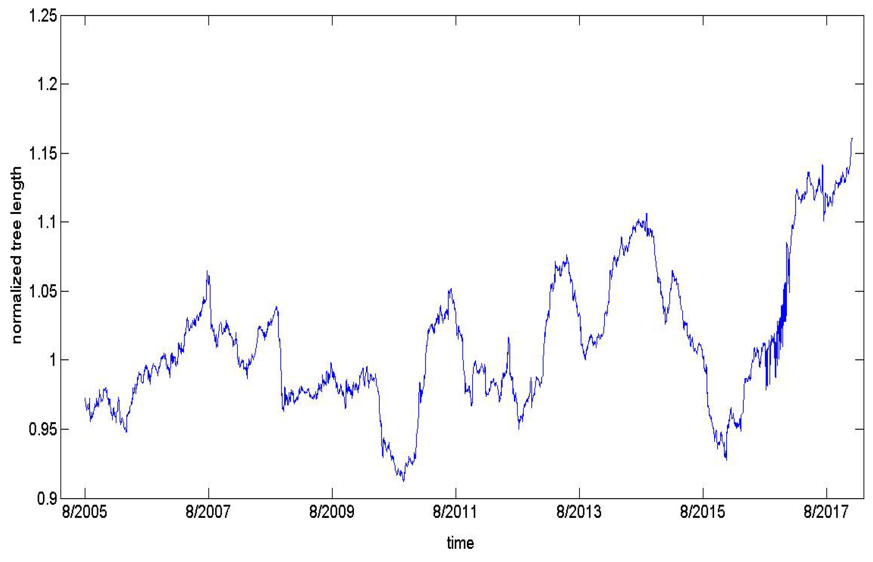
This paper employs a moving window correlation coefficient to compute the relationship between FX markets. To guarantee the statistical reliability, we choose the window length $\omega =150$ and roll forward at $\tau =1$ intervals. We analyze dynamic FX networks properties from the index of normalized tree length based on Formula (3), and the results are shown in Figure 1.

It can be seen from Figure 1 that the initial period of normalized tree length is followed by slow increasing tendency. When the sub-prime mortgage crisis broke out in August 2007, the normalized tree length dropped slightly. Since then, the normalized tree length had experienced a stationary period. When the European debt crisis broke out in 2010, the normalized tree length dropped sharply again. Afterwards, the normalized tree length had gone through a steady period of growth. In November 2015, the CNY belongs to an SDR currency basket, which is decided by the International Monetary Fund (IMF). The normalized tree length dropped to its lowest point once again. Henceforth, the normalized tree length had experienced an upward growth period. Therefore, we can find that the European debt crisis and the CNY join the special drawing rights have a significant impact on the FX network.

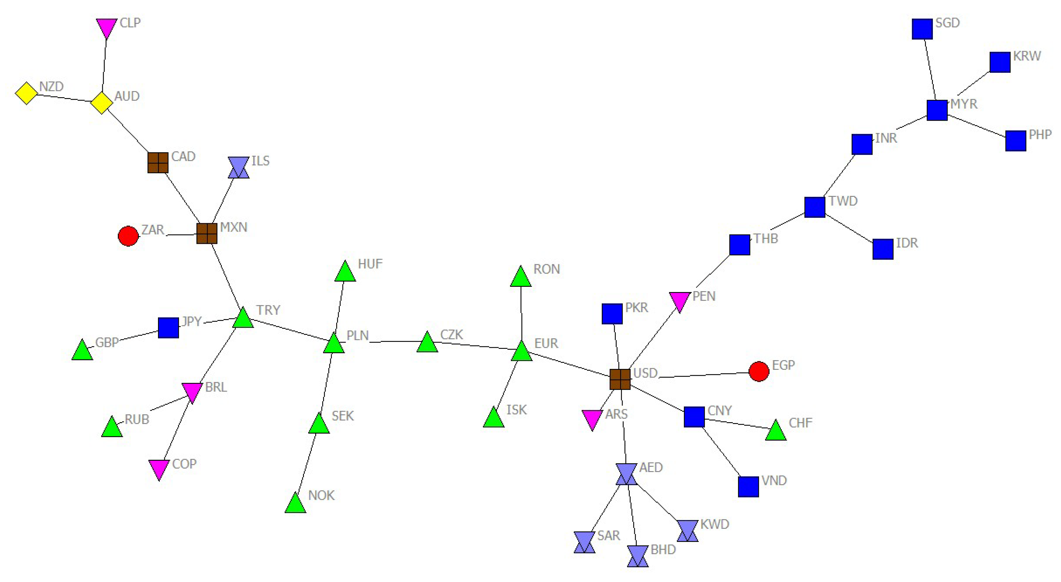
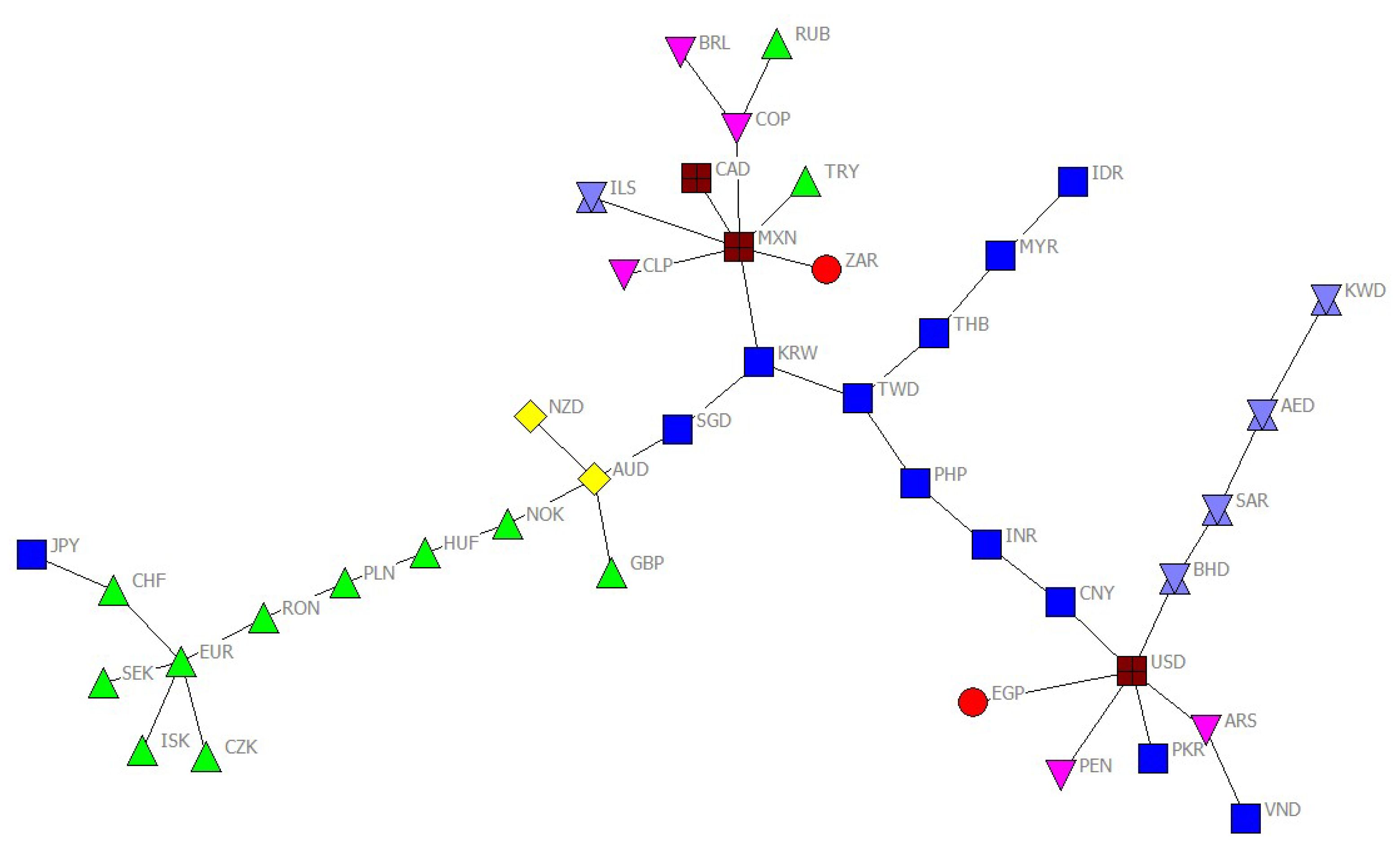
Considering the fact that the events (for example, sub-prime crisis, European debt crisis and the CNY join the special drawing rights) have a significant effect on FX markets, this paper selects three periods as representatives of major events and displays their networks in Figure 2, Figure 3 and Figure 4.

Figure 2 identifies the situation of FX markets during the sub-prime crises. It can find that (1) the USD is at the center of the FX network, which is directly linked with currencies from four continents (i.e., Africa, Asia, Europe, and Middle East); (2) three international currencies (i.e., USD, CNY and EUR) are linked together in the FX market, and USD is at their center; and (3) most of the currencies are connected together based on geography, such as the currencies of CNY, VND, TWD, MYR and SGD being in the Asian cluster. The currencies of EUR, NOK, SEK, PLN, CZK and HUF are in the European cluster. The currencies of BHD, AED, KWD and SAR are in the Middle East cluster. The currencies of BRL, CLP and COP are in the South America cluster. The currencies of AUD and NZD are in the Oceania cluster.

Compared with Figure 2, it can learn from Figure 3, which identifies the situation of FX markets during the European debt crises. (1) The USD is also at the center of the FX network, while there are more connecting nodes (i.e., Africa, Asia, Europe, Middle East and South America). (2) The European cluster still remains in the FX network, while their currencies are more aggregated. (3) The Asian cluster also exists in the FX network, but their structure and position are altered because of the financial crisis.

Compared with Figure 2 and Figure 3, it can learn from Figure 4, which identifies the situation of FX markets during the event of the CNY joining the special drawing rights. (1) The USD is not the only currency with more links in the FX network, and the EUR and MXN also have more connections. (2) The Asian cluster remains in the network, and the currencies of Asian are more aggregated. (3) The currencies of GBP, AUD, NZD and SGD are linked together because they all come from the Commonwealth countries.

Overall, this paper makes some conclusions as follows: (1) USD has a predominant position in the global currency market, but its dominance is decreasing because the status of other economies is rising. (2) The currencies of European are more closely and relatively stably linked during the periods of European debt crises and the event that the CNY joins the special drawing rights. This may be due to the fact that the EUR has the strongest influence in the European monetary system. (3) The currencies of Asian are more closely linked during the period in the event that the CNY joins the special drawing rights. This may be caused by the fact that the CNY has been regionalized in the process of promoting internationalization. (4) In addition to the ILS, the currencies in the Middle East form a cluster and connect to the US dollar. This could be ascribed to the fact that the Middle East are oil-producing countries and have a large amount of USD, and their currencies are pegged to the USD. (5) The currencies in the Oceania form a cluster. A possible interpretation is that they come from Commonwealth countries with the same political and cultural background.

Furthermore, this paper investigates the relationship between the normalized tree length (NTL) and market phenomena (moving window return and volatility of FX market index, which is calculated by Formulas (11) and (12)). Market phenomena are instructive of how the global FX market acts. In this paper, we consider the USD as the representative of the market index. Because it has been found that the USD has the dominant position in all of the periods, and its trend can better reflect the conditions of the global FX market.

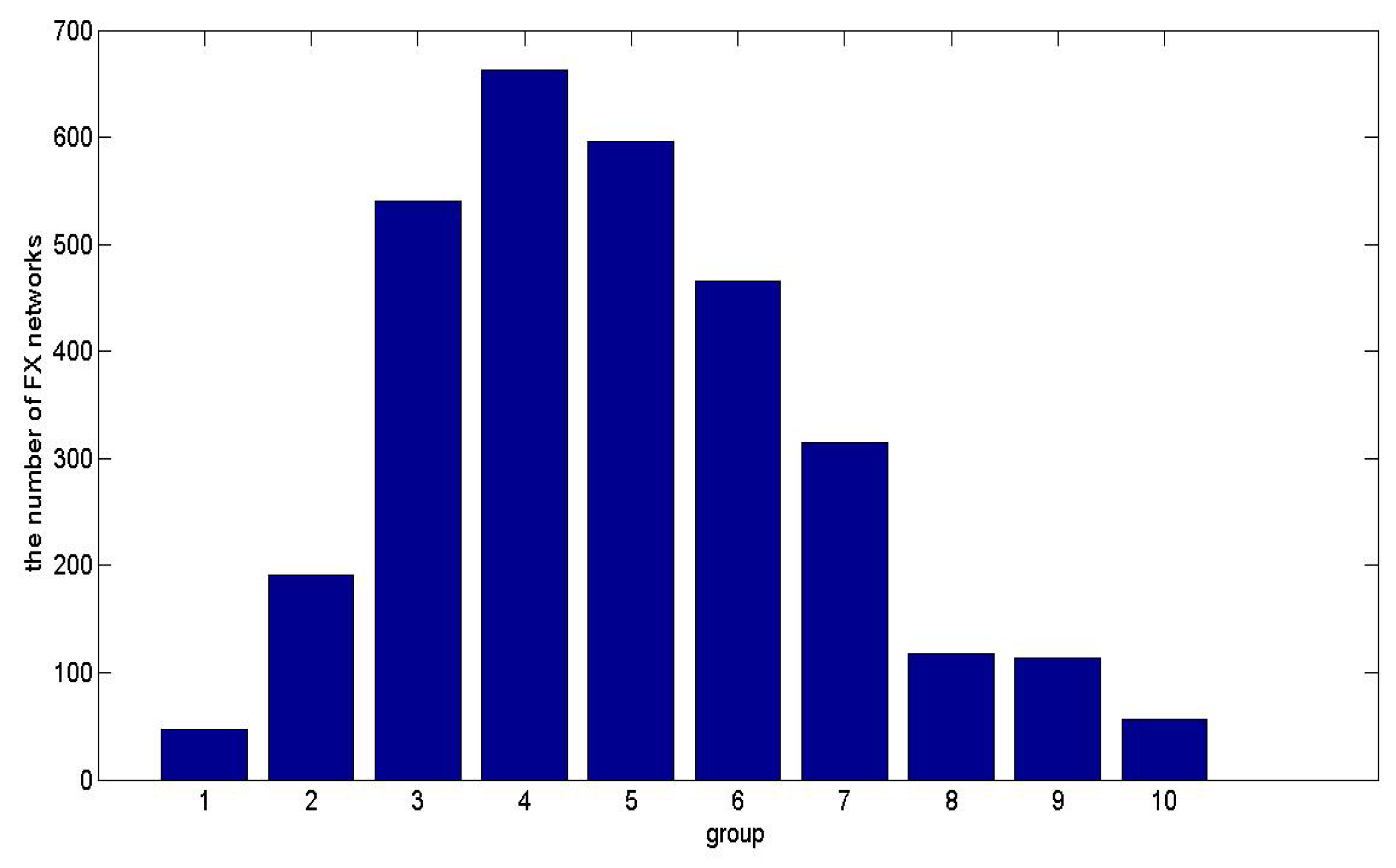
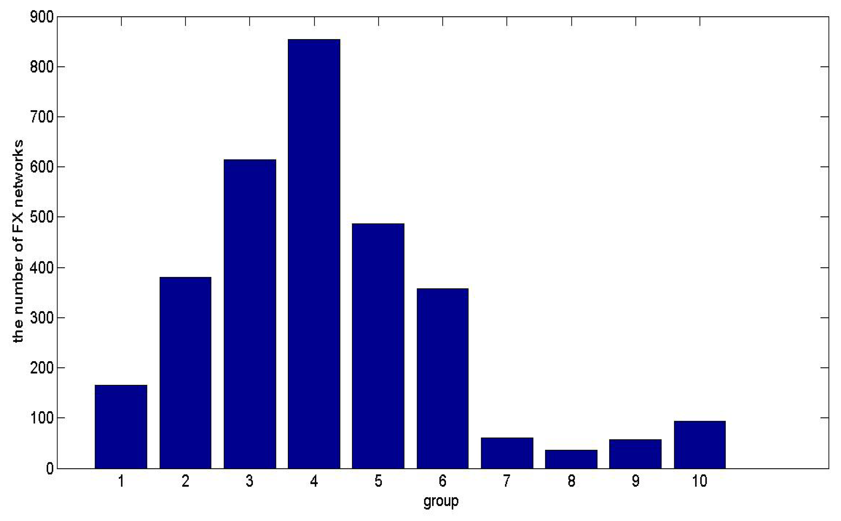
For the convenience of analysis, we divided the average return of the FX market index into 10 equal groups, and the trend from group 1 to group 10 represents the return of FX market index from the lowest to the highest value. Then, we count the quantity of networks corresponding to each group, and the results are shown in Figure 5.

As can be seen from Figure 5, we can find that (1) group 4 (with the mean value of the FX market index return varies from −0.000310 to −0.000007) has 662 FX networks, which is the largest in all groups, and (2) the quantity of FX networks, which belong to high or low value of the average FX market index’s return, is the smallest.

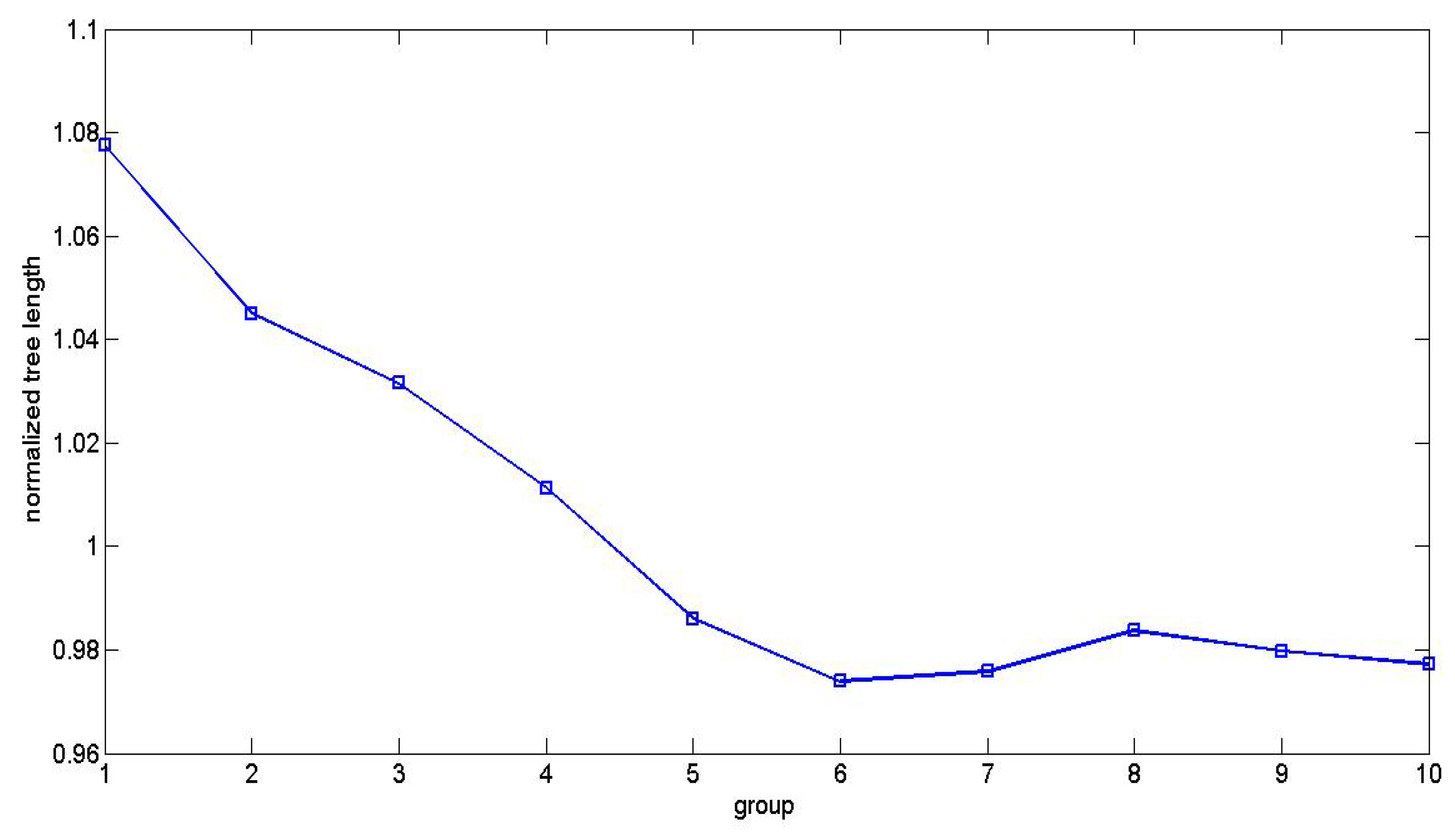
Furthermore, we calculate the mean value of the normalized tree length (NTL) of the corresponding network for each group, and the results are shown in Figure 6.

Figure 6 shows that there is a complex relationship between the NTL with the FX market index’s return. We can discover an increasing tendency of the NTL from group 1 to group 2 (the NTL’s mean value is from 0.978572 to 1.025761), and we then find a decreasing tendency of the NTL from group 2 to group 10 (the NTL’s mean value is from 1.025761 to 0.995016). It indicates that the FX network structure becomes looser at first and then becomes denser as the FX return rises.

Meanwhile, we split the average return volatility of the FX market index into 10 equal groups, and the trend from group 1 to group 10 represents the return volatility of the FX market index from the lowest to the highest value. Then, we calculate the quantity of networks corresponding to each group, and the results are shown in Figure 7.

It can be seen from Figure 7 that (1) the quantity of FX networks, which is attributed to group 4 (with volatility varies from 0.004423 to 0.005178), is the largest in all groups; (2) the number of FX networks with low volatility are more than those of the FX networks with high volatility; and (3) the quantity of groups 7 to 10 (with volatility varies from 0.002146 to 0.004420) contains the smaller FX networks.

In addition, we compute the mean value of the NTL of the corresponding network for each group, and the results are shown in Figure 8.

Figure 8 shows that there is a negative relationship between the NTL with the average return volatility of the FX market index. We can discover a decreasing tendency of the normalized tree length from group 1 with the smallest volatility (the NTL’s mean value is 1.077535) to group 10 with the largest volatility group (the NTL’s mean value is 0.977163). This means that the FX network structure turns denser, when FX market index volatility increases.

Overall, it can discover that the normalized tree length plays a role in identifying crises and is negatively correlated with the market return and volatility. Regulators can judge the possibility of the currency crisis and formulate relevant preventive measures according to the relationship between the NTL and market phenomena. This provides a new method for financial risk management.

3.2.2. Degree Distribution

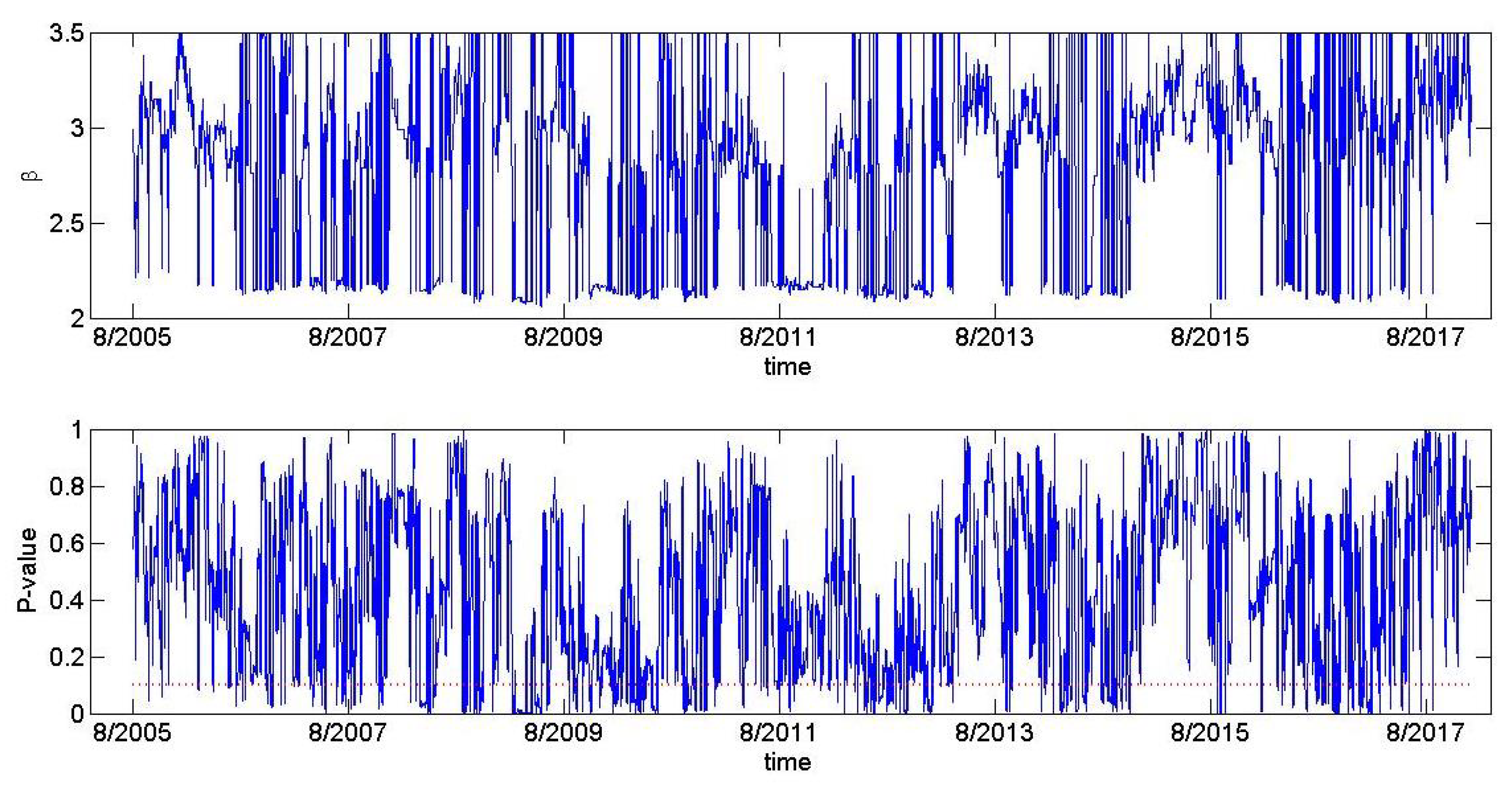
This paper analyzes the degree distribution of the FX network according to Formula (6), and Figure 9 displays the power-law exponent and the corresponding p-value.

As can be seen from Figure 9, the estimated power-law exponent varies from 2.06 to 3.50. Even though a small number of p-values are no more than 0.1, this paper can find that 83.41% of the FX network follows a power-law distribution. That is to say, a few nodes (such as USD) in the network occupy most of the edges, while the majority of nodes have a small number of edges. Therefore, these few nodes dominate the operation of the FX market.

3.2.3. Centrality Analysis

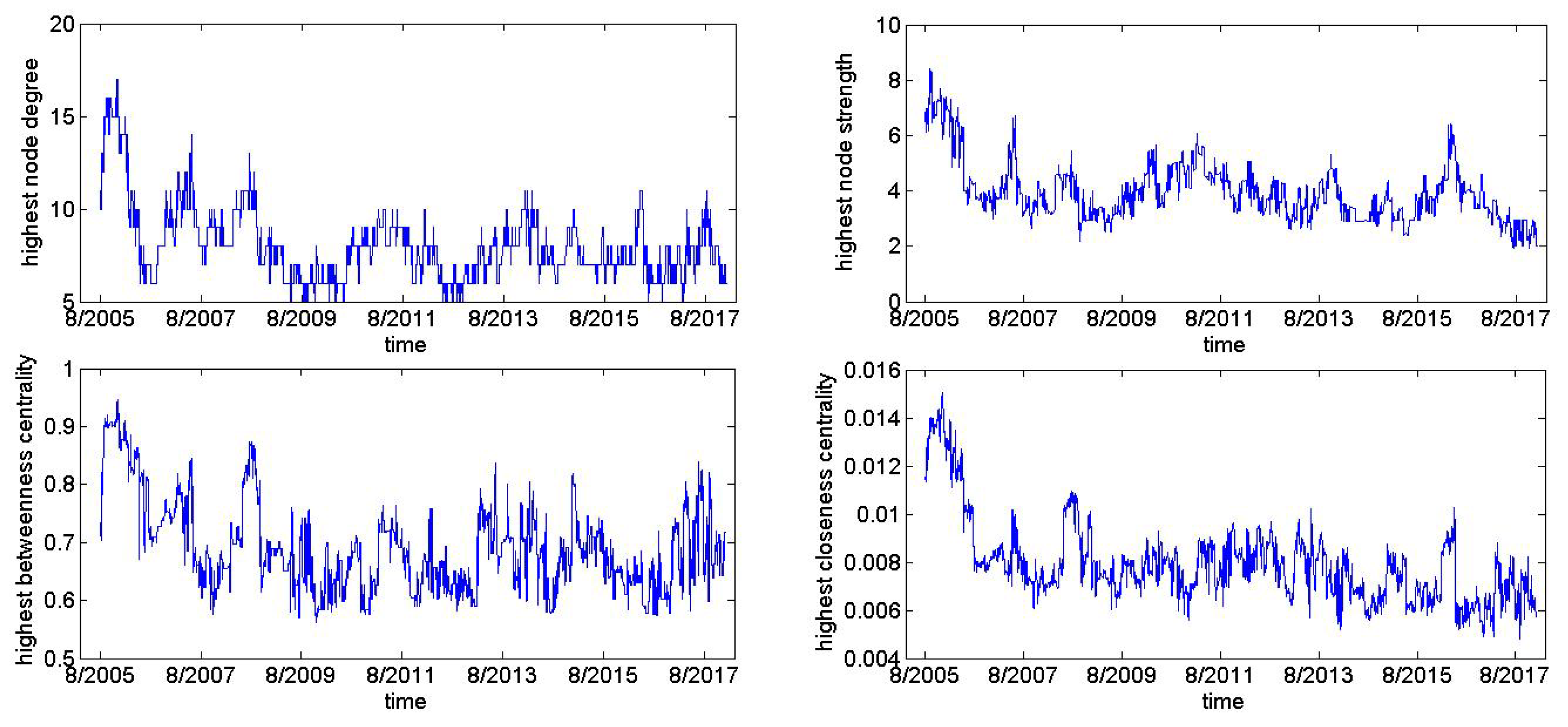
Centrality analysis is employed to measure the key nodes in the network. In practice, we choose four commonly used centrality measures, i.e., node degree, node strength, betweenness centrality and closeness centrality measures, which is calculated by Formulas (4), (5), (7) and (8). In addition, the results are shown in Figure 10.

It can be seen from Figure 10 that the four centrality measurements mentioned above vary from 5 to 17, from 1.9168 to 8.4200, from 0.5615 to 0.9462 and from 0.0048 to 0.0150, respectively. In addition, it shows a downward trend.

After analyzing the central analysis of the time-varying FX networks, it can find that the USD was not always in the center of the FX network. Some currencies are more influential than the USD for some periods. Therefore, this paper computes the occurrences of important nodes in each period. The results are shown in

Table 2. Top 10 foreign exchange (FX) markets ranked by the highest centrality measures.

Highest Node Degree		Highest Node Strength		Highest Betweenness Centrality		Highest Closeness Centrality
Currency	Frequency	Currency	Frequency	Currency	Frequency	Currency	Frequency
USD	2519	USD	1393	USD	1921	USD	1346
EUR	337	MXN	337	EUR	553	EUR	786
MXN	212	CNY	193	PLN	132	PLN	242
AUD	164	SAR	164	HUF	113	CNY	107
MYR	148	AUD	154	ZAR	65	HUF	94
CNY	102	AED	147	PHP	65	PHP	92
PLN	68	MYR	135	TRY	60	TWD	78
TRT	50	CZK	108	CNY	36	NOK	55
HUF	36	PLN	105	MXN	31	INR	50
KRW	27	HUF	100	TWD	28	CZK	33

.

Table 2 displays the top 10 FX markets ranked by the highest centrality measures in each period. It can find that the ranking of top ten FX markets has a minor differences for different highest centrality measures. However, USD is the most influential currency, which is in line with its economic status. Meanwhile, this paper believes that EUR is the second most influential currency, which is consistent with the position of the EUR in the international monetary system. In addition, CNY (By calculating the average ranking of four central measures, we can find that CNY ranks third.) is the third most influential currency from a comprehensive point of four indicators. This may be related to the increasing international status of the CNY. Therefore, this paper finds that the USD, EUR and CNY are the three most influencing currencies.

Furthermore, this paper studies the relationship between the centrality measures and market phenomena (return, and return volatility) by Pearson correlation coefficients. In addition, the results are shown as follows.

Table 3. Summarize the correlation coefficients between FX returns and centrality measures.

	The Quantity of $\mathit{\rho }\left(\mathit{k},\mathit{r}\right)$	The Quantity of $\mathit{\rho }\left(\mathit{s},\mathit{r}\right)$	The Quantity of $\mathit{\rho }\left(\mathit{b},\mathit{r}\right)$	The Quantity of $\mathit{\rho }\left(\mathit{c},\mathit{r}\right)$
0.40∼0.59	1	2	1	0
0.20∼0.39	1	8	3	3
0.00∼0.19	19	14	15	28
−0.19∼0.00	16	13	18	10
−0.39∼$-0.20$	3	2	4	0
$-0.59$∼$-0.40$	1	2	0	0
Significant positive	17	21	18	29
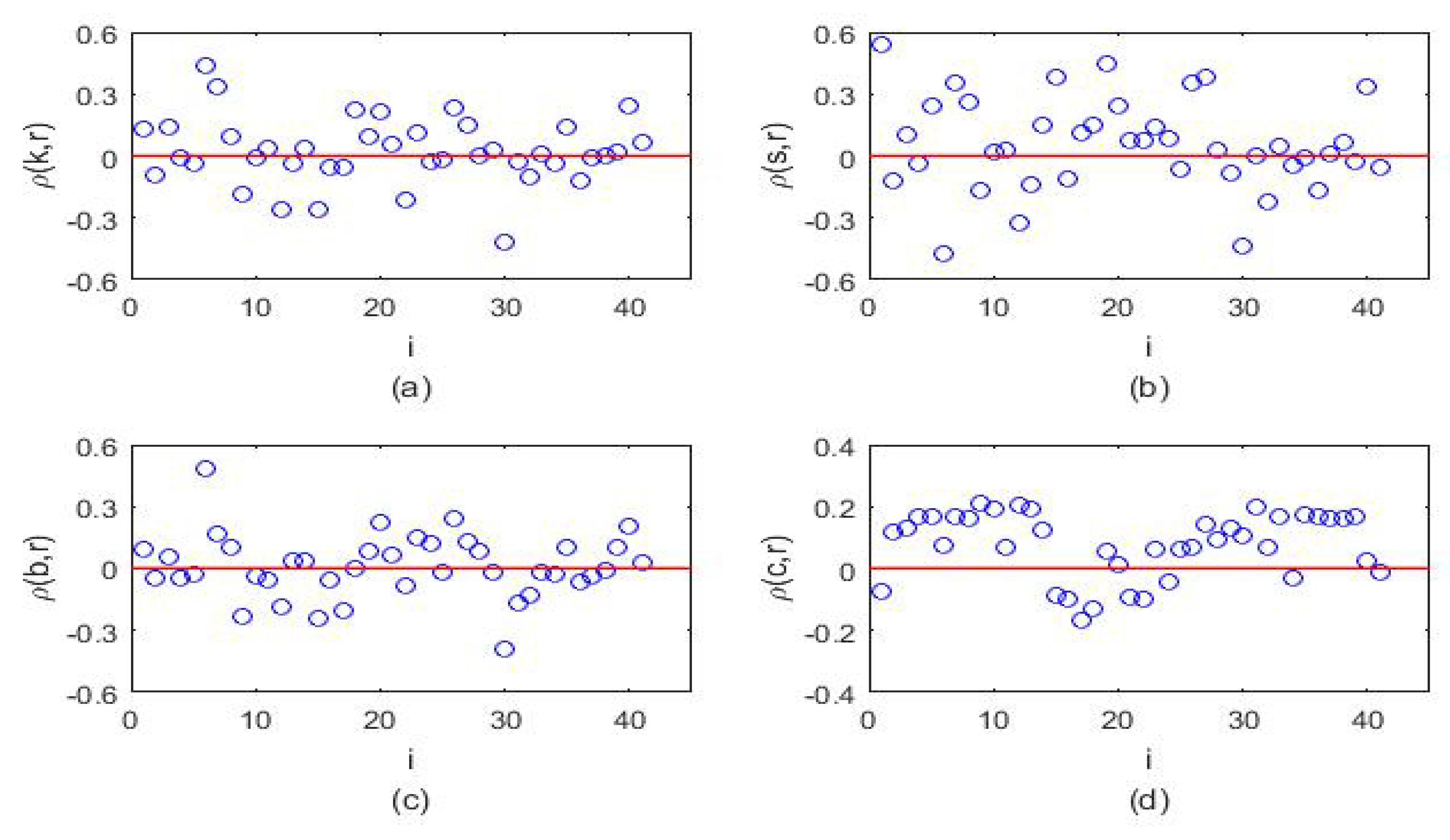
Significant negative	14	14	16	9

summarizes the Pearson correlation coefficients between each pair of FX return and centrality measures, and the results are displayed in Figure 11. We can discover that 17 FX markets’ return (41.46% of them) significantly positively correlated to their node degrees, 21 FX markets’ return (51.22% of them) significantly positively correlates to their node strengths, 18 FX markets’ return (43.90% of them) significantly positively correlates to their betweenness centrality, and 29 FX markets’ return (70.73% of them) significantly positively correlates to their closeness centrality. In total, we find that FX returns are positively correlated to their centrality measures.

Table 4. Summarize the correlation coefficients between FX volatility and centrality measures.

	The Quantity of $\mathit{\rho }\left(\mathit{k},\mathit{\sigma }\right)$	The Quantity of $\mathit{\rho }\left(\mathit{s},\mathit{\sigma }\right)$	The Quantity of $\mathit{\rho }\left(\mathit{b},\mathit{\sigma }\right)$	The Quantity of $\mathit{\rho }\left(\mathit{c},\mathit{\sigma }\right)$
0.40∼0.59	1	1	2	0
0.20∼0.39	8	8	6	0
0.00∼0.19	5	8	9	28
−0.19∼0.00	22	11	19	13
−0.39∼−0.20	5	5	5	0
−0.59∼−0.40	0	6	0	0
−0.79∼−0.60	0	2	0	0
Significant positive	14	16	16	18
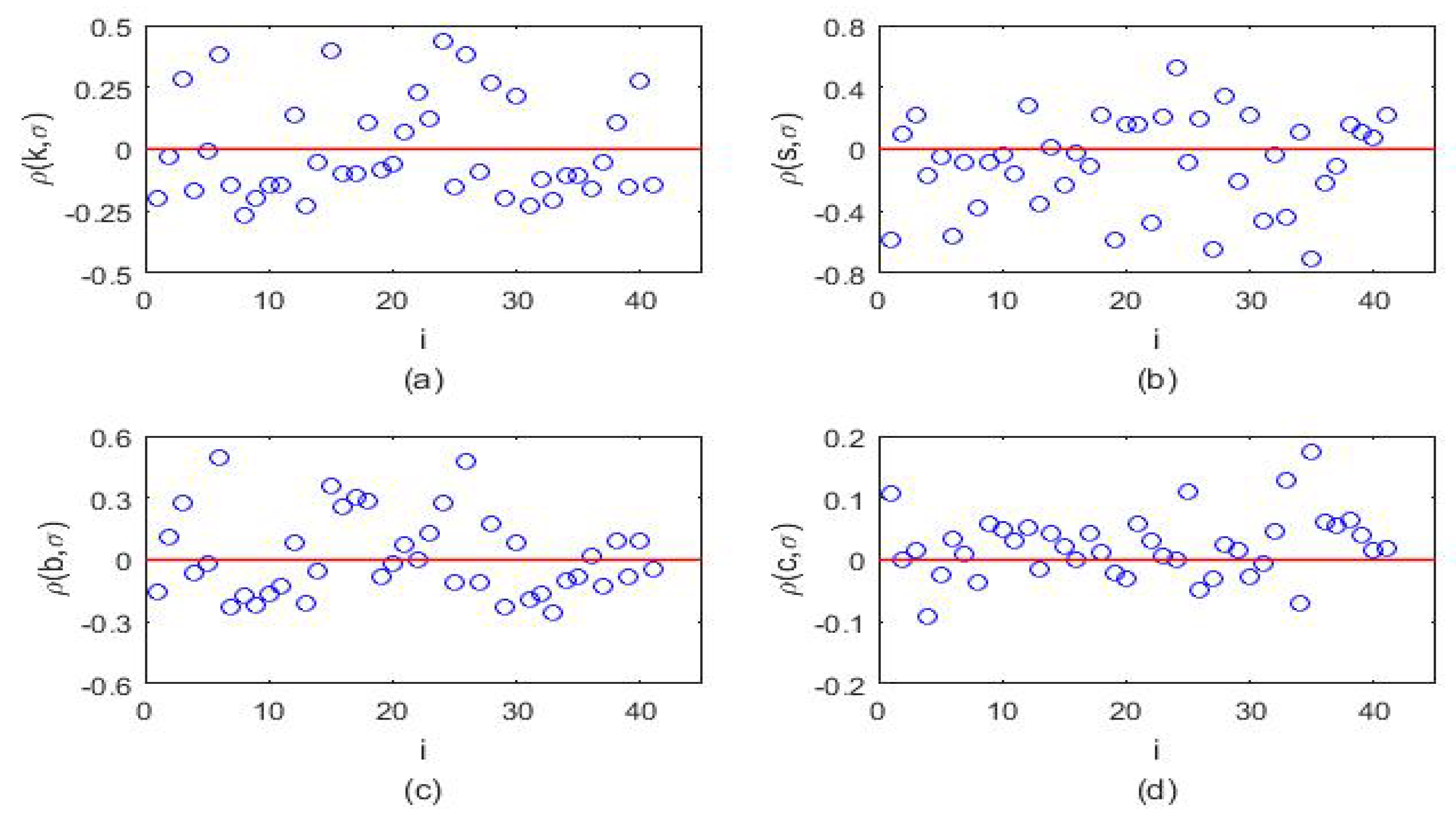
Significant negative	26	23	21	6

summarizes the Pearson correlation coefficients between each pair of FX return volatility and centrality measures, and the results are expressed as Figure 12. We can find that 26 FX markets’ volatility (63.41% of them) significantly negatively correlated to their node degrees, 23 FX markets’ volatility (56.10% of them) significantly negatively correlated to their node strengths, 21 FX markets’ volatility (51.22% of them) significantly negatively to their betweenness centrality, and 18 FX markets’ volatility (43.90% of them) significantly positively correlated to their closeness centrality. In total, it can find that FX volatility is negatively correlated to their centrality measures.

From the above results, this paper can conclude that the majority of FX markets’ return significantly positively correlates to their centrality measures, and the volatility significantly negatively correlates to their centrality measures. When major events occur in the FX markets, we can focus on important FX rates based on the relationship between market phenomena and centrality measures. In addition, we can classify the portfolio investment from the relationship between market phenomena and node centrality measures. It can provide a novel method for the government to manage risk and investment in the FX market.

3.2.4. Survival Ratio Analysis

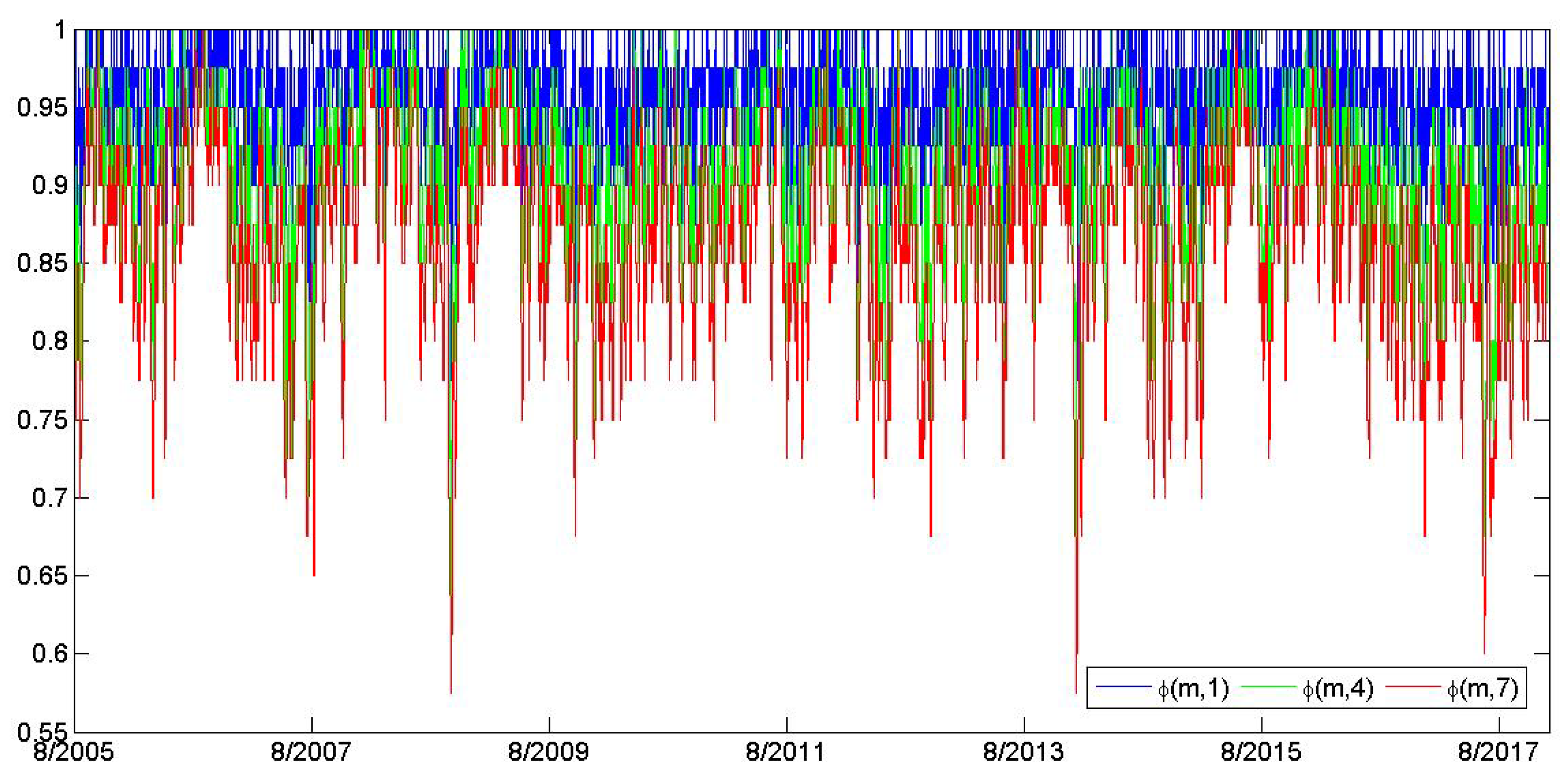
The survival ratio is computed by Formulas (9) and (10), which is examining the FX network’s consecutive stability. Figure 13 presents the survival ratio of the FX network at different steps. This paper calculates the steps of 1, 4, 7.

As can be seen from Figure 13, the mean of the single-step survival ratio series is 0.95, which indicates that a large number of the edges of the FX networks survive from time t to t + 1. i.e., most of the edges in the adjacent two FX networks have not changed, and only about 5% of edges has changed. In other words, from the perspective of the short-term evolution of the network, the FX market has a robust relationship that can hardly be broken.

From the view of multiple survival ratio analysis, each multiple survival ratio (MSR) curve decreases quickly over time, which denotes that the stability of the global FX network has dropped sharply with time. However, each MSR curve has a constant interval, which means that part of the global FX network topology (such as the Middle East region) has remained constant and it shows a good stability.

4. Conclusions

This paper employs a moving window Pearson correlation coefficient in the daily closing prices of 41 FX markets from January 2005 to December 2017. Then, we adopt the MST method to build the corresponding networks. The dynamic topology properties of networks are characterized by the normalized tree length, node degree distributions, centrality measures and edge survival ratios.

Some basic findings of this paper can be concluded as follows: (1) the sub-prime mortgage crisis, the European debt crisis and the CNY joining the special drawing rights make NTL decrease sharply. Meanwhile, the USD has a predominant position in the FX market of these three periods, but its dominance is decreasing due to the status of other economies rising. The FX rates of European are more closely and relatively stably linked during the periods of European debt crises because the EUR has the strongest influence in the European monetary system. The currencies of Asian are more closely linked during the period of the event when the CNY joins the special drawing rights. This may be caused by the fact that CNY has been regionalized in the process of promoting internationalization. Furthermore, it can find that the NTL are negative against the FX market return and volatility with the corresponding window. Regulators can judge the possibility of the currency crisis and formulate relevant preventive measures according to the relationship between the NTL and the returns and risks of the FX market index. (2) The degree distribution of the 83% networks show scale-free characteristic and the power-law exponent varies from 2.06 to 3.50, which means that the FX market is a typical heterogeneous market, and a few hub nodes play key roles in the market. (3) The USD, EUR and CNY are the three most powerful currencies. Moreover, we further discover that the majority of FX markets’ return significantly positively correlate to their centrality measures, and the volatility significantly negatively correlates to their centrality measures. (4) Single-step survive reveals that 95% of the links of the FX network survives between adjacent time periods, and multi-step survive denotes that the robustness of FX networks decreases quickly as the time elapses.

References

- Mendez, R.P. Harnessing the global foreign currency market: Proposal for a foreign currency exchange (FXE). Rev. Int. Polit. Econ. 1996, 3, 498–512. [Google Scholar] [CrossRef]
- Andersen, T.G.; Bollerslev, T.; Diebold, F.X.; Labys, P. The distribution of realized exchange rate volatility. J. Am. Stat. Assoc. 2001, 96, 42–55. [Google Scholar] [CrossRef]
- Mák, I.; Páles, J. The role of the FX swap market in the hungarian financial system. Gen. Inf. 2009, 4, 24–34. [Google Scholar]
- Lane, P.R.; Milesi-Ferretti, G.M. External wealth, the trade balance, and the real exchange rate. Eur. Econ. Rev. 2002, 46, 1049–1071. [Google Scholar] [CrossRef] [Green Version]
- Debelle, G. The Australian foreign exchange market. Econ. Rec. 2006, 22, 4–11. [Google Scholar]
- Hau, H. The exchange rate effect of multi-currency risk arbitrage. Soc. Sci. Electron. Publ. 2009, 47, 304–331. [Google Scholar] [CrossRef]
- Francis, B.; Paolo, V. An empirical study of portfolio-balance and information effects of order flow on exchange rates. J. Int. Money Financ. 2010, 29, 504–524. [Google Scholar] [Green Version]
- Kotzé, A.; Oosthuizen, R.; Pindza, E. Implied and local volatility surfaces for south african index and foreign exchange options. J. R. Financ. Manag. 2015, 8, 43–82. [Google Scholar] [CrossRef]
- Malone, S.; Gramacy, R.; Ter Horst, E. Timing foreign exchange markets. Econometrics 2016, 4, 15. [Google Scholar] [CrossRef]
- Huang, C.; Cao, J.; Wen, F.; Yang, X. Stability analysis of sir model with distributed delay on complex networks. PLoS ONE 2016, 11, e0158813. [Google Scholar] [CrossRef]
- Huang, C.; Liu, B. New studies on dynamic analysis of inertial neural networks involving non-reduced order method. Neurocomputing 2019, 325, 283–287. [Google Scholar]
- Yang, C.; Huang, L.; Li, F. Exponential synchronization control of discontinuous nonautonomous networks and autonomous coupled networks. Complexity 2018, 2018, 6164786. [Google Scholar] [CrossRef]
- Huang, C.; Liu, B.; Tian, X.; Yang, L.; Zhang, X. Global convergence on asymptotically almost periodic sicnns with nonlinear decay functions. Neural Process. Lett. 2019, 49, 625–641. [Google Scholar]
- Long, X.; Gong, S. New results on stability of Nicholson’s blowflies equation with multiple pairs of time-varying delays. Appl. Math. Lett. 2019. [Google Scholar] [CrossRef]
- Zhu, Q.; Huang, C.; Yang, X. Exponential stability for stochastic jumping bam neural networks with time-varying and distributed delays. Nonlinear Anal. Hybrid Syst. 2011, 5, 52–77. [Google Scholar] [CrossRef]
- Huang, C.; Su, R.; Cao, J.; Xiao, S. Asymptotically stable high-order neutral cellular neural networks with proportional delays and d operators. Math. Comput. Simul. 2019. [Google Scholar] [CrossRef]
- Song, C.; Fei, S.; Cao, J.; Huang, C. Robust synchronization of fractional-order uncertain chaotic systems based on output feedback sliding mode control. Mathematics 2019, 7, 599. [Google Scholar] [CrossRef]
- Hu, H.; Yuan, X.; Huang, L.; Huang, C. Global dynamics of an SIRS model with demographics and transfer from infectious to susceptible on heterogeneous networks. Math. Biosci. Eng. 2019, 16, 5729–5749. [Google Scholar] [CrossRef]
- Tan, Y.; Huang, C.; Sun, B.; Wang, T. Dynamics of a class of delayed reaction-diffusion systems with Neumann boundary condition. J. Math. Anal. Appl. 2018, 458, 1115–1130. [Google Scholar]
- Huang, C.; Zhang, H.; Cao, J.; Hu, H. Stability and Hopf bifurcation of a delayed prey-predator model with disease in the predator. Int. J. Bifurcat. Chaos 2019, 29, 1950091. [Google Scholar] [CrossRef]
- Huang, C.; Zhang, H.; Huang, L. Almost periodicity analysis for a delayed Nicholson’s blowflies model with nonlinear density-dependent mortality term. Commun. Pur. Appl. Anal. 2019, 18, 3337–3349. [Google Scholar] [CrossRef]
- Huang, C.; Qiao, Y.; Huang, L.; Agarwal, R. Dynamical behaviors of a food-chain model with stage structure and time delays. Adv. Differ. Equ. 2018, 2018. [Google Scholar] [CrossRef]
- Emma, M.I. An analysis of extreme movements of exchange rates of the main currencies traded in the foreign exchange market. Appl. Econ. 2012, 44, 4631–4637. [Google Scholar]
- Hussein, M.S. Event-Based Microscopic Analysis of the FX Market. Ph.D. Thesis, University of Essex, Colchester, UK, 2013; pp. 1–202. [Google Scholar]
- Holtgrave, M.; Onay, M. Success through trust, control, and learning? Contrasting the drivers of SME performance between different modes of foreign market entry. Adm. Sci. 2017, 7, 9. [Google Scholar] [CrossRef]
- Nie, C.X.; Song, F.T. Relationship between entropy and dimension of financial correlation-based network. Entropy 2018, 20, 177. [Google Scholar] [CrossRef]
- Hayward, R. Foreign exchange speculation: An event study. Int. J. Financ. Stud. 2018, 6, 22. [Google Scholar] [CrossRef]
- Niu, H.L.; Zhang, L. Nonlinear Multiscale Entropy and Recurrence Quantification Analysis of Foreign Exchange Markets Efficiency. Entropy 2018, 20, 17. [Google Scholar] [CrossRef]
- Zhou, G.Y.; Yan, X.X.; Luo, S.M. Financial Security and Optimal Scale of Foreign Exchange Reserve in China. Sustainability 2018, 10, 1724. [Google Scholar] [CrossRef]
- Mcdonald, M.; Suleman, O.; Williams, S.; Howison, S.; Johnson, N.F. Detecting a currency’s dominance or dependence using foreign exchange network trees. Phys. Rev. E Stat. Nonlinear Soft Matter Phys. 2005, 72, 046106. [Google Scholar] [CrossRef] [PubMed]
- Guillermo, J.O.; David, M. Cross-country hierarchical strcture and currency crisis. Int. J. Mod. Phys. C 2006, 17, 333–341. [Google Scholar]
- Keskin, M.; Deviren, B.; Kocakaplan, Y. Topology of the correlation networks among major currencies using hierarchical structure methods. Phys. A Stat. Mech. Appl. 2011, 390, 719–730. [Google Scholar] [CrossRef]
- Wu, X.Y.; Zheng, Z.G. Hierarchical cluster-tendency analysis of the group structure in the foreign exchange market. Front. Phys. 2013, 8, 451–460. [Google Scholar] [CrossRef]
- Jiang, J.; Ma, K.; Cai, X. Scaling and correlations in foreign exchange market. Phys. A Stat. Mech. Appl. 2007, 375, 274–280. [Google Scholar] [CrossRef]
- Mizuno, T.; Takayasu, H.; Takayasu, M. Correlation networks among currencies. Phys. A Stat. Mech. Appl. 2006, 364, 336–342. [Google Scholar] [CrossRef] [Green Version]
- Kwapien, J.; Gworek, S.; Drozdz, S. Structure and evolution of the foreign exchange networks. Acta Phys. Pol. 2009, 40, 1–23. [Google Scholar]
- Mai, Y.; Chen, H.; Zou, J.Z.; Li, S.P. Currency co-movement and network correlation structure of foreign exchange market. Phys. A Stat. Mech. Appl. 2018, 492, 65–74. [Google Scholar] [CrossRef]
- Wang, G.J.; Xie, C. Tail dependence structure of the foreign exchange market: A network view. Expert Syst. Appl. 2015, 46, 164–179. [Google Scholar] [CrossRef]
- Cao, G.X.; Zhang, Q.; Li, Q.C. Causal relationship between the global foreign exchange market based on complex networks and entropy theory. Chaos Solitons Fract. 2017, 99, 36–44. [Google Scholar] [CrossRef]
- Fenn, D.J.; Porter, M.A.; Mcdonald, M.; Williams, S.; Johnson, N.F.; Jones, N.S. Dynamic communities in multichannel data: An application to the foreign exchange market during the 2007–2008 credit crisis. Chaos 2009, 19, 033119. [Google Scholar] [CrossRef]
- Wang, G.J.; Xie, C.; Han, F.; Sun, B. Similarity measure and topology evolution of foreign exchange markets using dynamic time warping method: Evidence from minimal spanning tree. Phys. A Stat. Mech. Appl. 2012, 391, 4136–4146. [Google Scholar] [CrossRef]
- Fenn, D.J.; Porter, M.A.; Mucha, P.J.; Mcdonald, M.; Williams, S.; Johnson, N.F.; Jones, N.S. Dynamical clustering of exchange rates. Quant. Financ. 2012, 12, 1493–1520. [Google Scholar] [CrossRef] [Green Version]
- Suzuki, T. The Renminbi exchange rate reform and its implications for Asian markets. China Q. Int. Strateg. Stud. 2016, 2, 485–506. [Google Scholar] [CrossRef]
- Takatoshi, I. A new financial order in Asia: Will a RMB bloc emerge? J. Int. Money Financ. 2017, 74, 1–57. [Google Scholar]
- Flaschel, P.; Hartmann, F.; Malikane, C.; Proaño, C.R. A behavioral macroeconomic model of exchange rate fluctuations with complex market expectations formation. Comput. Econ. 2015, 45, 669–691. [Google Scholar] [CrossRef]
- Bekaert, G.; Hodrick, R.J. Characterizing predictable components in excess returns on equity and foreign exchange markets. J. Financ. 1992, 47, 467–509. [Google Scholar] [CrossRef]
- Christiansen, C. Intertemporal risk-return trade-off in foreign exchange rates. J. Int. Financ. Mark. Inst. Money 2011, 21, 535–549. [Google Scholar] [CrossRef]
- Humala, A.; Rodriguez, G. Some stylized facts of return in the foreign exchange and stock markets in Peru. Stud. Econ. Financ. 2011, 30, 139–158. [Google Scholar] [CrossRef]
- Juselius, K.; Assenmacher, K. Real exchange rate persistence and the excess return puzzle: The case of Switzerland versus the US. J. Appl. Econometr. 2017, 32, 1145–1155. [Google Scholar] [CrossRef]
- Abuelfadl, M. Individual foreign exchange investors, return predictability and market timing. Ann. Financ. Econ. 2017, 12, 238–256. [Google Scholar] [CrossRef]
- Zhou, B. High-frequency data and volatility in foreign-exchange rates. J. Bus. Econ. Stat. 1996, 14, 45–52. [Google Scholar]
- Mcgroarty, F.; Gwilym, O.A.; Thomas, S. The role of private information in return volatility, bid-ask spreads and price levels in the foreign exchange market. J. Int. Financ. Mark. Inst. Money 2009, 19, 387–401. [Google Scholar] [CrossRef]
- Dumas, B.; Solnik, B. The world price of foreign exchange risk. J. Financ. 2012, 50, 445–479. [Google Scholar] [CrossRef]
- Daigler, R.T.; Hibbert, A.M.; Pavlova, I. Examining the return-volatility relation for foreign exchange: Evidence from the Euro VIX. J. Futures Mark. 2014, 34, 74–92. [Google Scholar] [CrossRef]
- Menkhoff, L.; Sarno, L.; Schmeling, M.; Schrimpf, A. Information flows in foreign exchange markets: Dissecting customer currency trades. J. Financ. 2016, 71, 601–634. [Google Scholar] [CrossRef]
- Bolboaca, S.D.; Jäntschi, L. Pearson versus Spearman, Kendall’s tau correlation analysis on structure-activity relationships of biologic active compounds. Leonardo. J. Sci. 2006, 5, 179–200. [Google Scholar]
- Mantegna, R.N. Hierarchical structure in financial markets. Eur. Phys. J. B Condens. Matter Complex Syst. 1999, 11, 193–197. [Google Scholar] [CrossRef] [Green Version]
- Kruskal, J.B. On the shortest spanning subtree of a graph and the traveling salesman problem. Proc. Am. Math. Soc. 1956, 7, 48–50. [Google Scholar] [CrossRef]
- Onnela, J.P.; Chakraborti, A.; Kaski, K.; Kertész, J. Dynamic asset trees and black monday. Phys. A Stat. Mech. Appl. 2003, 324, 247–252. [Google Scholar] [CrossRef]
- Adamic, L.A.; Lukose, R.M.; Puniyani, A.R.; Huberman, B.A. Search in power-law networks. Phys. Rev. E Stat. Nonlinear Soft Matter Phys. 2001, 64, 046135. [Google Scholar] [CrossRef] [Green Version]
- Yook, S.H.; Jeong, H.; Barabási, A.L. Modeling the internet’s large-scale topology. Proc. Natl. Acad. Sci. USA 2002, 99, 13382–13386. [Google Scholar] [CrossRef]
- Huang, W.Q.; Yao, S.; Zhuang, X.T.; Yuan, Y. Dynamic asset trees in the US stock market: Structure variation and market phenomena. Chaos Solitons Fract. 2017, 94, 44–53. [Google Scholar] [CrossRef]
- Hai, X.D.; Ren, G.J.; Yu, Y.G.; Xu, C.H. Adaptive Pinning Synchronization of Fractional Complex Networks with Impulses and Reaction–Diffusion Terms. Mathematics 2019, 7, 405. [Google Scholar] [CrossRef]
- Rodríguez, L.C.; Alarcón, R.L. Use of Enumerative Combinatorics for proving the applicability of an asymptotic stability result on discrete-time SIS epidemics in complex networks. Mathematics 2019, 30, 30. [Google Scholar] [CrossRef]
- Jäntschi, L. A Test Detecting the Outliers for Continuous Distributions Based on the Cumulative Distribution Function of the Data Being Tested. Symmetry 2019, 11, 835. [Google Scholar] [CrossRef]
- Clauset, A.; Shalizi, C.R.; Newman, M.E.J. Power-law distributions in empirical data. Siam Rev. 2009, 51, 661–703. [Google Scholar] [CrossRef]
- Wang, G.J.; Xie, C.; Chen, Y.J.; Chen, S. Statistical properties of the foreign exchange network at different time scales: Evidence from detrended cross-correlation coefficient and minimum spanning tree. Entropy 2013, 15, 1643–1662. [Google Scholar] [CrossRef]
- Wang, G.J.; Xie, C.; Zhang, P.; Han, F.; Chen, S. Dynamics of foreign exchange networks: a time-varying copula approach. Discret. Dyn. Nat. Soc. 2014, 2014, 170921. [Google Scholar] [CrossRef]
- Yoon, J.; Blumer, A.; Lee, K. An algorithm for modularity analysis of directed and weighted biological networks based on edge-betweenness centrality. Bioinformatics 2006, 22, 3106–3108. [Google Scholar] [CrossRef] [PubMed] [Green Version]
- Costenbader, E.; Valente, T.W. The stability of centrality measures when networks are sampled. Soc. Netw. 2003, 25, 283–307. [Google Scholar] [CrossRef]
- Jang, W.; Lee, J.; Chang, W. Currency crises and the evolution of foreign exchange market: Evidence from minimum spanning tree. Phys. A Stat. Mech. Appl. 2011, 390, 707–718. [Google Scholar] [CrossRef]
Figure 1.
The normalized tree length of the foreign exchange (FX) network in each period.
Figure 2.
FX network during 18 March 2008–21 October 2008, as a representative of sub-prime crises. FX markets from the same region are labeled with the same color and shape (i.e., Africa, red circles; Asia, blue squares; Europe, green up triangles; Middle East, light blue things; North America, gray boxes; South America, pink down triangles; Oceania, yellow diamonds) henceforth.
Figure 3.
FX network during 22 February 2010–24 September 2010, as a representative of European debt crises.
Figure 4.
FX network during 12 May 2015–15 December 2015, as a representative event of the CNY joining the special drawing rights.
Figure 5.
The quantity of FX networks in each group according to the average return of the FX market index with the corresponding time window.
Figure 6.
The mean value of the normalized tree length in each group according to the average return of the FX market index with the corresponding time window.
Figure 7.
The quantity of FX networks in each group according to the average return volatility of the FX market index with the corresponding time window.
Figure 8.
The mean value of the normalized tree length in each group according to the average return volatility of the FX market index with the corresponding time window.
Figure 9.
In the top panel, we estimated power-law exponent of degree distribution at a different time. In the bottom panel, we estimated the corresponding p-value of the power-law exponent, and the red line denotes the value of 0.1. If the p-value is over 0.1, we accepted the power-law hypothesis, otherwise it was rejected.
Figure 10.
The highest centrality measures in the FX network.
Figure 11.
Pearson correlation coefficients between return and (a) node degree; (b) node strength; (c) betweenness centrality; (d) closeness centrality for each FX market.
Figure 12.
Pearson correlation coefficients between volatility and (a) node degree; (b) node strength; (c) betweenness centrality; (d) closeness centrality for each FX market.
Figure 13.
Survival ratio under different steps.