A New Divergence Measure of Pythagorean Fuzzy Sets Based on Belief Function and Its Application in Medical Diagnosis

Abstract

As the extension of the fuzzy sets (FSs) theory, the intuitionistic fuzzy sets (IFSs) play an important role in handling the uncertainty under the uncertain environments. The Pythagoreanfuzzy sets (PFSs) proposed by Yager in 2013 can deal with more uncertain situations than intuitionistic fuzzy sets because of its larger range of describing the membership grades. How to measure the distance of Pythagorean fuzzy sets is still an open issue. Jensen–Shannon divergence is a useful distance measure in the probability distribution space. In order to efficiently deal with uncertainty in practical applications, this paper proposes a new divergence measure of Pythagorean fuzzy sets, which is based on the belief function in Dempster–Shafer evidence theory, and is called PFSDM distance. It describes the Pythagorean fuzzy sets in the form of basic probability assignments (BPAs) and calculates the divergence of BPAs to get the divergence of PFSs, which is the step in establishing a link between the PFSs and BPAs. Since the proposed method combines the characters of belief function and divergence, it has a more powerful resolution than other existing methods. Additionally, an improved algorithm using PFSDM distance is proposed in medical diagnosis, which can avoid producing counter-intuitive results especially when a data conflict exists. The proposed method and the magnified algorithm are both demonstrated to be rational and practical in applications.

1. Introduction

With the development of fuzzy mathematics, medical diagnosis has addressed more and more attention from the research society of applied computer mathematics. In the diagnostic process of medical profession, improving the processing capacity of various uncertain and inconsistent information and achieving more accurate decision-making have become the major challenges in the development of medical diagnosis [1,2,3]. Up to now, the process of medical diagnosis is driven by various theoretical studies, such as fuzzy sets theory [4,5,6], intuitionistic fuzzy sets [7,8,9,10], interval-valued intuitionistic fuzzy sets [11,12,13], and quantum decision [14,15,16].

It is well known that medical diagnosis is an effective and reasonable way to handle the problem of uncertainty. Decision theory [17,18,19] has been widely applied in this field, containing a variety of theories and methods. For instance, evidence theory and its extension [20,21,22], evidential reasoning [23,24], D numbers theory [25], R numbers theory [26,27], Z numbers theory [28,29], and other hybrid methods have been used to research it from lots of aspects. The rationality and practicality of these methods have also been proven by their employment in applications, such as strategy selection [30,31,32,33,34], decision-making [35,36,37,38,39], prediction [40,41,42], and fault diagnosis [43,44]. In addition, Zadeh presented a useful theory in 1965, the fuzzy set (FS) theory [45], which drives a big step forward in decision theory. Atanassov’s intuitionistic fuzzy sets (IFSs) [46] proposed and Yager’s Pythagorean fuzzy sets (PFSs) [47] are two extensions of a fuzzy set which make use of the membership degree, non-membership degree, and the hesitancy to preciously express the uncertainty. Among them, Pythagorean fuzzy set has a larger range of expressing the uncertainy than intuitionistic fuzzy set [48,49]. Hence, the Pythagorean fuzzy set was chosen to apply for medical diagnosis in this paper.

Distance measure plays a vital role in pattern recognition, information fusion, decision-making, and other fields. The fuzzy set theory and intuitionistic fuzzy sets have been proposed for many years and their distance measurements [50,51,52] have matured compared with Pythagorean fuzzy sets. There are some useful distances for IFS after suffering the practice and the application. For instance, the Euclidean distance [53], the Hamming distance [53], and the Hausdorff metric [54] are the most widely applied distances of IFS. The distance measurement of PFSs is still an open issue, which attracts many researchers to explore the distance measurement of PFSs and its related applications. A general distance measurement of PFSs was proposed by Chen [55], is an extension of Euclidean distance and Hamming distance, and generates a reasonable result in multiple-criteria decision analysis. Wei and Wei [56] proposed a PFS measurement method based on cosine function and applied it to medical diagnosis to achieve an ideal result. Later on, Xiao [57] presented a distance measurement of PFSs based on divergence, called PFSJS distance. Among these methods of measure distance of PFSs, membership, non-membership and hesitancy are calculated based on the same weights. It is well known that the hesitancy expresses the uncertainty of membership and non-membership, so finding a proper method to distribute hesitancy to membership and non-membership can more reasonably handle the distance of PFSs. The basic probability assignment (BPA) in evidence theory presented by Dempster–Shafer [58,59] unifies uncertainty in a new set, and can handle various uncertainty reasonably. Song [60] presented a divergence measure of belief function based on Kullback–Leibler (KL) divergence [61] and Deng entropy [62], which has better results when dealing with the distance between BPAs with greater uncertainty. This paper proposes a new method to describe the PFSs in the form of BPAs, and uses an improverd divergence measurement of BPAs based on Jensen–Shannon divergence to measure the distance of PFSs. This method applied to medical diagnosis can not only get more intuitive results when the high conflicts appear in several symptoms between patients and diseases but also make higher resolution in different results.

According to the above, the structure of this article is as follows:

• The related concepts and properties of Pythagorean fuzzy set (PFS), basic probability assignment (BPA), the Jensen–Shannon divergence, and some widely applied methods of measuring distance are introduced.
• A new divergence measure of PFSs is proposed, which is called PFSDM distance. Its measurement is divided into three stages. The first is establishing a link between PFSs and BPAs. In addition, then, an improved method is proposed to measure the divergence of PFSs represented as BPAs. The third is proving the properties of PFSDM distance and expressing the feasibility and merits of the proposed method using numerical examples.
• The medical diagnosis algorithm based on Xiao’s method [57] is magnified and compares the new algorithm with other existing methods to prove its practicability.
• The merits and uses of the PFSDM distance are summarized and the future direction of algorithm improvement is expected.

2. Preliminaries

In this section, the first subsection introduced the definition of Pythagorean fuzzy sets [47,48]. The main idea of basic probability assignment (BPA), Dempster–Shafer evidence theory [58,59] is in the second subsection. Some concepts of divergence are in the third subsection. In the last subsection, some existing methods for measuring the distance of PFSs are displayed.

2.1. Pythagorean Fuzzy Sets

Definition 1.

Let X be a limited universe of discourse. An intuitionistic fuzzy set (IFS) [46] M in X is defined by

$$M=\{\langle x,{\mu }_M\left(x\right),v_M\left(x\right)\rangle \mid x\in X\},$$

(1)

where ${\mu }_M\left(x\right):X\to [0,1]$ represents the degree of support for membership of the $x\in X$ of IFS, and $v_M\left(x\right):X\to [0,1]$ represents the degree of support for non-membership of the $x\in X$ of IFS, with the condition that $0\le {\mu }_M\left(x\right)+v_M\left(x\right)\le 1$. and the hesitancy function ${\pi }_M\left(x\right)$ of IFS reflecting the uncertainty of membership and non-membership is defined by

$${\pi }_M\left(x\right)=1-{\mu }_M\left(x\right)-v_M\left(x\right).$$

(2)

Definition 2.

Let x be a limited universe of discourse. A Pythagorean fuzzy set (PFS) [47,48] M in X is defined by

$$M=\left\{〈x,M_Y\left(x\right),M_N\left(x\right)〉|x\in X\right\},$$

(3)

where $M_Y\left(x\right):X\to [0,1]$ represents the degree of support for membership of the $x\in X$ of PFS, and $M_N\left(x\right):X\to [0,1]$ represents the degree of support for non-membership of the $x\in X$ of PFS, with the condition that $0\le M_Y^2\left(x\right)+M_N^2\left(x\right)\le 1$. and the hesitancy function $M_H\left(x\right)$ of PFS reflecting the uncertainty of membership and non-membership is defined by

$$M_H\left(x\right)=\sqrt{1-M_Y^2\left(x\right)+M_N^2\left(x\right)}.$$

(4)

The membership and the non-membership of PFS also can be expressed by another way. A pair of values $r\left(x\right)$ and $d\left(x\right)$ for each $x\in X$ are used to represent the membership and non-membership as follows:

$$M_Y\left(x\right)=r_M\left(x\right)Cos\left({\theta }_M\left(x\right)\right)M_N\left(x\right)=r_M\left(x\right)Sin\left({\theta }_M\left(x\right)\right),$$

(5)

where $\theta \left(x\right)=(1-d\left(x\right))\frac{\pi }{2}=Arctan(M_N\left(x\right)/M_Y\left(x\right))$. Here, we see that $\theta \left(x\right)$ is expressed as radians and $\theta \left(x\right)\in [0,\frac{\pi }{2}]$. In addition, $M_H\left(x\right)=\sqrt{1-r^2\left(x\right)}$.

Property 1.

([49]) Let B and C be two PFSs in X, then

• $B\subseteq C$ if $\forall x\in X,B_Y\left(x\right)\le C_Y\left(x\right)$ and $B_N\left(x\right)\ge C_N\left(x\right)$,
• $B=C$ if $\forall x\in X,B_Y\left(x\right)=C_Y\left(x\right)$ and $B_N\left(x\right)=C_N\left(x\right)$,
• $B\cap C=\left\{〈x,min\left[B_Y\left(x\right),C_Y\left(x\right)\right]\right.$,$\left.\left.max\left[B_N\left(x\right),C_N\left(x\right)\right]\right)|x\in X\right\}$,
• $B\cup C=\left\{\left(x,max\left[B_Y\left(x\right),C_Y\left(x\right)\right],min\left[B_N\left(x\right),C_N\left(x\right)\right]\right)|x\in X\right]$,
• $B·C=\left\{〈x,B_Y\left(x\right)C_Y\left(x\right),{\left(B_N^2\left(x\right)+C_N^2\left(x\right)-B_N^2\left(x\right)C_N^2\left(x\right)\right)}^{\frac{1}{2}}〉|x\in X\right\}$,
• $B^n=\left\{\left(x,B_Y^n\left(x\right),{\left(1-\left(1-B_N^2{\left(x\right)}^n\right)\right)}^{\frac{1}{2}}\right)|x\in X\right\}$.

2.2. Dempster–Shafer Evidence Theory

The Dempster–Shafer evidence theory [58,59] is proposed to deal with conditions that are weaker than Bayes probability [63,64], which can directly express uncertainty and unknown information [65,66], so that it has been widely used in various applications, FMEA [67,68,69], evidential reasoning [70,71,72], evaluation [73], target recognition [74], industrial alarm system [75,76], and others [77,78].

Definition 3.

Θ is the set of N elements which represent mutually exclusive and exhaustive hypotheses. Θ is the frame of discernment [58,59]:

$$\Theta =\left\{H_1,H_2,\cdots ,H_i,\cdots ,H_N\right\}.$$

(6)

The power set of Θ is denoted by $2^{\Theta }$, and

$$2^{\Theta }=\left\{\varnothing ,\left\{H_1\right\},\cdots ,\left\{H_n\right\},\left\{H_1,H_2\right\},\cdots ,\left\{H_1,\cdots ,H_N\right\}\right\},$$

(7)

where ∅ is an empty set.

Definition 4.

A mass function [58,59] m, also called as BPA, is a mapping of $2^{\Theta }$, defined as follows:

$$m:2^{\Theta }\to [0,1],$$

(8)

which satisfies the following conditions:

$$m(\varnothing )=0\sum _{A\in 2^{\ominus }}m\left(A\right)=10\le m\left(A\right)\le 1A\in 2^{\Theta }.$$

(9)

The mass $m\left(A\right)$ represents how strongly the evidence supports A [79,80,81].

2.3. Divergence Measure

Definition 5.

Given two probabilities distribution $A=\{A\left(x_1\right),A\left(x_2\right),\cdots ,A\left(x_n\right)\}$ and $B=\{B\left(x_1\right),B\left(x_2\right),\cdots ,B\left(x_n\right)\}$.

Kullback–Leibler divergence [61] between A and B is defined as:

$${Div}_{KL}(A,B)=\sum _{i=1}^{n}A\left(x_i\right){log}_2\left(\frac{A\left(x_i\right)}{B\left(x_i\right)}\right)$$

(10)

with ${\sum }_{i=1}^{n}A\left(x_i\right)={\sum }_{i=1}^{n}B\left(x_i\right)=1$.

The Kullback–Leibler also has some disadvantages of its properties, and one of them is that it doesn’t satisfy the commutative property:

$${Div}_{KL}(A,B)\ne {Div}_{KL}(B,A).$$

(11)

In order to realize the commutation in the distance measure, the Jensen–Shannon divergence is an adaptive choice.

Definition 6.

Given two probabilities distribution $A=\{A\left(x_1\right),A\left(x_2\right),\cdots ,A\left(x_n\right)\}$ and $B=\{B\left(x_1\right),B\left(x_2\right),\cdots ,B\left(x_n\right)\}$.

Jensen–Shannon divergence [82] between A and B is defined as:

$$J{S}_{AB}=\frac{Di{v}_{KL}(A,\frac{A+B}{2})+Di{v}_{KL}(B,\frac{A+B}{2})}{2}=H\left(\frac{A+B}{2}\right)-\frac{H\left(A\right)}{2}-\frac{H\left(B\right)}{2},$$

(12)

where $H\left(A\right)=-{\sum }_{i=1}^{n}A\left(x_i\right)logA\left(x_i\right)$ and ${\sum }_{i=1}^{n}A\left(x_i\right)={\sum }_{i=1}^{n}B\left(x_i\right)=1$.

Song’s divergence [60] is used to measure the belief function, which is capable of processing uncertainty efficiently in a highly fuzzy environment by applying the thinking of Deng entropy [62].

Definition 7.

([60]) Given two basic probability assignments (BPAs) $m_1$ and $m_2$, the divergence between $m_1$ and $m_2$ is defined as follows:

$$D_{SD}\left(m_1,m_2\right)=\sum _i\frac{1}{2^{\left|F_i\right|-1}}{m}_1\left(F_i\right)log\left(\frac{m_1\left(F_i\right)}{m_2\left(F_i\right)}\right),$$

(13)

where the $F_i$ holds on ${\sum }_{i=1}^{2^{\Theta }-1}m\left(F_i\right)=1$, which is the power subset of frame of discernment Θ and $\left|F_i\right|$ is the cardinal number of $F_i$.

It is obvious that $D_{SD}(m_1,m_2)\ne D_{SD}(m_2,m_1)$. In order to realize the commutative property, a divergence measurement based on Song’s divergence is defined as follows:

$$D_{SDM}(m_1,m_2)={\tilde{D}}_{SDM}(m_2,m_1)=\frac{D_{SD}\left(m_1,m_2\right)+D_{SD}\left(m_2,m_1\right)}{2}.$$

(14)

Because of thinking of the number of subsets of the mass function and averagely distributing the BPAs to these subsets, Song’s divergence is more reasonable than others when the basic probability assignments of non-singleton powers sets $F_i$ are larger.

2.4. Distance Measure of Pythagorean Fuzzy Sets

The Euclidean distance [53] and the Hamming distance [53] are the most widely applied distances, and Chen proposed a generalized distance measure of PFS [55], which is the extension of Hamming distance and Euclidean distance.

Definition 8.

Let X be a limited universe of discourse, and M and N are two PFSs. Chen’s distance [55] measure between PFSs M and N denoted as $D_C(M,N)$ is defined as:

$$D_C(M,N)={\left[\frac{1}{2}(\mid M_Y^2\left(x\right)-N_Y^2\left(x\right){\mid }^{\beta }+\mid M_N^2\left(x\right)-N_N^2\left(x\right){\mid }^{\beta }+\mid M_H^2\left(x\right)-N_H^2\left(x\right){\mid }^{\beta })\right]}^{\frac{1}{\beta }},$$

(15)

where β holds on $\beta \ge 1$ is called the distance parameter. As the extension of the Hamming distance and Euclidean distance, if $\beta =1$ and $\beta =2$, the Chen’s distance is equal to Hamming distance and Euclidean distance, respectively:

• if $\beta =1$,
  $D_C(M,N)=D_{Hm}(M,N)=\left[\frac{1}{2}(\mid M_Y^2\left(x\right)-N_Y^2\left(x\right)\mid +\mid M_N^2\left(x\right)-N_N^2\left(x\right)\mid +\mid M_H^2\left(x\right)-N_H^2\left(x\right)\mid )\right]$,
• if $\beta =2$,
  $D_C(M,N)=D_E(M,N)={\left[\frac{1}{2}({(M_Y^2\left(x\right)-N_Y^2\left(x\right))}^2+{(M_N^2\left(x\right)-N_N^2\left(x\right))}^2+{(M_H^2\left(x\right)-N_H^2\left(x\right))}^2)\right]}^{\frac{1}{2}}$.

In the application of distance measure, the universe of discourse always has many properties. Xiao extended them as the normalized distance and proposed a divergence measure of PFSs called PFSJS based on the Jensen–Shannon divergence, which is the first work to calculate the distance of PFSs using divergence.

Let $X=\{x_1,x_2,\cdots ,x_n\}$ be a limited universe of discourse, two PFSs

$M=\{\langle x_i,M_Y\left(x_i\right),M_N\left(x_i\right)\rangle \mid x_i\in X\}$ and $N=\{\langle x_i,N_Y\left(x_i\right),N_N\left(x_i\right)\rangle \mid x_i\in X\}$ are in X.

Definition 9.

The normalized Hamming distance [57] denoted as ${\tilde{D}}_{Hm}(M,N)$ is defined as:

$${\tilde{D}}_{Hm}(M,N)=\frac{1}{2n}\sum _{i=1}^n(\mid M_Y^2\left(x\right)-N_Y^2\left(x\right)\mid +\mid M_N^2\left(x\right)-N_N^2\left(x\right)\mid +\mid M_H^2\left(x\right)-N_H^2\left(x\right)\mid ).$$

The normalized Euclidean distance [57] denoted as ${\tilde{D}}_E(M,N)$ is defined as:

$${\tilde{D}}_E(M,N)=\frac{1}{n}\sum _{i=1}^n{\left[\frac{1}{2}({(M_Y^2\left(x\right)-N_Y^2\left(x\right))}^2+{(M_N^2\left(x\right)-N_N^2\left(x\right))}^2+{(M_H^2\left(x\right)-N_H^2\left(x\right))}^2)\right]}^{\frac{1}{2}}.$$

The normalized Chen’s distance [57] denoted as ${\tilde{D}}_C(M,N)$ is defined as:

$${\tilde{D}}_C(M,N)=\frac{1}{n}\sum _{i=1}^n{\left[\frac{1}{2}(\mid M_Y^2\left(x\right)-N_Y^2\left(x\right){\mid }^{\beta }+\mid M_N^2\left(x\right)-N_N^2\left(x\right){\mid }^{\beta }+\mid M_H^2\left(x\right)-N_H^2\left(x\right){\mid }^{\beta })\right]}^{\frac{1}{\beta }},$$

where $\beta \ge 1$

Definition 10.

The normalized divergence measurements of Pythagorean fuzzy sets denoted as PFSJS [57] of M and N are defined as follows:

$$\begin{array}{c}{\tilde{D}}_x(M,N)=\frac{1}{n}·\sum _{i=1}^n{D}_x(M,N)\hfill \\ =\frac{1}{n}\sum _{i=1}^n\sqrt{\frac{1}{2}\left[{\sum }_{\kappa }{M}_{\kappa }^2\left(x_i\right)log\left(\frac{2M_{\kappa }^2\left(x_i\right)}{M_{\kappa }^2\left(x_i\right)+N_{\kappa }^2\left(x_i\right)}\right)+{\sum }_{\kappa }{N}_{\kappa }^2\left(x_i\right)log\left(\frac{2N_{\kappa }^2\left(x_i\right)}{M_{\kappa }^2\left(x_i\right)+N_{\kappa }^2\left(x_i\right)}\right)\right]},\hfill \end{array}$$

(16)

where $\kappa \in \kappa \in \{Y,N,H\}$.

According to the existing methods for measuring the PFSs’ distance, what they have in common is that the weights of membership $A_Y\left(x\right)$ non-membership $A_N\left(x\right)$ and hesitancy $A_H\left(x\right)$ are considered to be the same when calculating distances. As is well known, the hesitancy represents the uncertainty of membership degree and non-membership degree, and the belief function in evidence theory can handle the uncertainty in a more proper way. Hence, if the ability of evidence theory to handle uncertainty is combined with the high resolution of divergence in distance measurement, the PFSs’ distance measurement will be further optimized. In the next section, a new divergence measure of PFSs is proposed based on belief function, which describes the PFSs in the form of BPAs and measures the distance of PFSs by calculating the divergence of BPAs.

3. A New Divergence Measure of PFSs

In this section, a new divergence measure of PFSs, called PFSDM distance, is proposed. The first subsection shows how PFS reasonably expressed in the form of BPA. A new improved method of BPAs’ divergence measure is introduced in the second subsection, and then the PFSDM distance and its properties is proposed. In the last subsection, some examples are used to prove its properties and demonstrate its feasibility by comparing with existing other methods.

3.1. PFS Is Expressed in the Form of BPA

In the evidence theory [58,59], the basic probability assignment (BPA) $m\left(A\right)$ represents the degree of evidence supporting A, and, according to Equations (6) and (7), the elements of power set of frame of discernment ($\Theta$) should satisfy ${\sum }_{A\in 2^{\theta }}m\left(A\right)=1$. Thus, the method of representing PFS in the form of BPA is shown as follows:

Definition 11.

Let X be a limited universe of discourse, according to the second form of PFS shown in Equation (5), a Pythagorean fuzzy set M in X is $M=\{\langle x,r_M\left(x\right)Cos\left({\theta }_M\left(x\right)\right),r_M\left(x\right)Sin\left({\theta }_M\left(x\right)\right)\rangle \mid x\in X\}$, the frame of discernment ${\Theta }_M$ of M and their basic probability assignments $m_p$ are defined as:

$${\Theta }_M=\{Y_M,N_M\},$$

(17)

• $m_p\left(Y_M\right)=r_M\left(x\right)Co{s}^2{\theta }_M\left(x\right)$,
• $m_p\left(N_M\right)=r_M\left(x\right)Si{n}^2{\theta }_M\left(x\right)$,
• $m_p\left(Y_M{N}_M\right)=1-r_M\left(x\right)$,
• $m_p\left(\varphi \right)=0$,

where $m_p\left(Y_M\right)$ represents the degree of evidence supporting membership of M. The $m_p\left(N_M\right)$ represents the degree of evidence supporting non-membership of M. The $m_p\left(Y_M{N}_M\right)$ represents the degree of evidence supporting membership and non-membership. Because the basic focal elements $Y_M$ and $N_M$ are totally exclusive, and the sum of them is equal to 1, they conform to the Dempster–Shafer evidence theory.

According to the meaning of $m_p\left(Y_M{N}_M\right)$ and the method of thinking of Deng entropy [62], it contains the degree of evidence supporting the elements of $\left\{Y_M\right\}$, $\left\{Y_N\right\}$ and $\left\{Y_M{Y}_N\right\}$, and Song [60] redistributes the degree of supporting $\left\{Y_M{N}_M\right\}$ averagely among the three elements when calculating the distance of BPAs in Equation (13).

3.2. A New Divergence Measure of PFSs

Jensen–Shannon divergence is widely used in distance measure of probability distributions, and in this subsection, we propose an improved divergence measure of BPA based on Song’s divergence and Jensen–Shannon divergence. In addition, a new divergence measure of PFSs and its properties are proposed, which is capable of distinguishing PFSs better.

Definition 12.

Let Θ be a frame of discernment $\Theta =\{A_1,A_2,\cdots ,A_n\}$, and the power set of Θ is $2^{\Theta }=\{\varnothing ,\left\{A_1\right\},\cdots ,\left\{A_n\right\},\{A_1,A2\},\cdots ,\{A_1,A_n\},\cdots ,\{A_1,\cdots ,A_n\}\}=\{\varnothing ,F_1,F_2,\cdots ,F_{2^n-1}\}$. The Jensen–Shannon divergence measure $D_{JS}(m_1,m_2)$ of two BPAs $m_1$, $m_2$ is defined as:

$$\begin{array}{cc}\hfill D_{JS}(m_1,m_2)& =\frac{1}{2}[D_{SD}(m_1,\frac{m_1+m_2}{2})+D_{SD}(m_2,\frac{m_2+m_1}{2})]\hfill \\ & =\frac{1}{2}[\sum _{F_i\in 2^{\theta }}\frac{1}{2^{\mid Fi\mid -1}}{m}_1\left(F_i\right)log\left(\frac{2m_1\left(F_i\right)}{m_1\left(F_i\right)+m_2\left(F_i\right)}\right)+\sum _{F_i\in 2^{\theta }}\frac{1}{2^{\mid Fi\mid -1}}{m}_2\left(F_i\right)log\left(\frac{2m_2\left(F_i\right)}{m_1\left(F_i\right)+m_2\left(F_i\right)}\right)],\hfill \end{array}$$

(18)

where $\mid F_i\mid$ is the cardinal number of $F_i$. In addition, just in case there’s a zero in the denominator, ${10}^{-8}$ is used to replace zero in the calculation.

The improved method satisfies the symmetry and considers the number of elements in the power set. In addition, then, substituting the PFSs in the form of BPAs into Equation (18) produces the new divergence measure of Pythagorean fuzzy sets.

Definition 13.

Let X be a limited universe of discourse, according to the second form of PFS shown in Equation (5), two Pythagorean fuzzy sets M and N in X are $M=\{\langle x,r_M\left(x\right)Cos\left({\theta }_M\left(x\right)\right),r_M\left(x\right)Sin\left({\theta }_M\left(x\right)\right)\rangle \mid x\in X\}$, $N=\{\langle x,r_N\left(x\right)Cos\left({\theta }_N\left(x\right)\right),r_N\left(x\right)Sin\left({\theta }_N\left(x\right)\right)\rangle \mid x\in X\}$. The divergence measure denoted as $D_{PFS}(M,N)$ is defined as follows:

$$\begin{array}{cc}\hfill D_{PFS}(M,N)=& \frac{1}{2}[r_M\left(x\right)Co{s}^2{\theta }_M\left(x\right)log\left(\frac{2r_M\left(x\right)Co{s}^2{\theta }_M\left(x\right)}{r_M\left(x\right)Co{s}^2{\theta }_M\left(x\right)+r_N\left(x\right)Co{s}^2{\theta }_N\left(x\right)}\right)+\hfill \\ & r_N\left(x\right)Co{s}^2{\theta }_N\left(x\right)log\left(\frac{2r_N\left(x\right)Co{s}^2{\theta }_N\left(x\right)}{r_M\left(x\right)Co{s}^2{\theta }_M\left(x\right)+r_N\left(x\right)Co{s}^2{\theta }_N\left(x\right)}\right)+\hfill \\ & r_M\left(x\right)Si{n}^2{\theta }_M\left(x\right)log\left(\frac{2r_M\left(x\right)Si{n}^2{\theta }_M\left(x\right)}{r_M\left(x\right)Si{n}^2{\theta }_M\left(x\right)+r_N\left(x\right)Si{n}^2{\theta }_N\left(x\right)}\right)+\hfill \\ & r_N\left(x\right)Si{n}^2{\theta }_N\left(x\right)log\left(\frac{2r_N\left(x\right)Si{n}^2{\theta }_N\left(x\right)}{r_M\left(x\right)Si{n}^2{\theta }_M\left(x\right)+r_N\left(x\right)Si{n}^2{\theta }_N\left(x\right)}\right)+\hfill \\ & \frac{1}{3}\left(1-r_M\left(x\right)\right)log\left(\frac{2(1-r_M\left(x\right))}{(1-r_M\left(x\right))+(1-r_N\left(x\right))}\right)+\hfill \\ & \frac{1}{3}\left(1-r_N\left(x\right)\right)log\left(\frac{2(1-r_N\left(x\right))}{(1-r_M\left(x\right))+(1-r_N\left(x\right))}\right)].\hfill \end{array}$$

(19)

In order to obtain higher resolution when making distance measurement, the divergence measure of PFSs, PFSDM distance, denoted as $D_{mp}(M,N)$, is defined by

$$D_{mp}(M,N)=\sqrt{D_{PFS}(M,N)}.$$

(20)

According to the properties of Jensen–Shannon divergence [82], the larger PFSDM distance, the more different PFSs, and the smaller PFSDM, the more similar PFSs. The properties of the PFSDM distance are displayed as follows:

Definition 14.

Let M and N be two PFSs in a limited universe of discourse $X=\{x_1,x_2,\cdots ,x_n\}$, where

$M=\left\{\langle x_i,r_M\left(x_i\right)Cos\left({\theta }_M\left(x_i\right)\right),r_M\left(x_i\right)Sin\left({\theta }_M\left(x_i\right)\right)\rangle \right\}$, $N=\left\{\langle x_i,r_N\left(x_i\right)Cos\left({\theta }_N\left(x_i\right)\right),r_N\left(x_i\right)Sin\left({\theta }_N\left(x_i\right)\right)\rangle \right\}$.

The normalized PFSDM distance, ${\tilde{D}}_{mp}(M,N)$, is defined as follows:

$$\begin{array}{cc}\hfill {\tilde{D}}_{mp}(M,N)=& \frac{1}{n}\sum _{i=1}^n\left\{\frac{1}{2}\right[r_M\left(x_i\right)Co{s}^2{\theta }_M\left(x_i\right)log\left(\frac{2r_M\left(x_i\right)Co{s}^2{\theta }_M\left(x_i\right)}{r_M\left(x_i\right)Co{s}^2{\theta }_M\left(x_i\right)+r_N\left(x_i\right)Co{s}^2{\theta }_N\left(x_i\right)}\right)+\hfill \\ & r_N\left(x_i\right)Co{s}^2{\theta }_N\left(x_i\right)log\left(\frac{2r_N\left(x_i\right)Co{s}^2{\theta }_N\left(x_i\right)}{r_M\left(x_i\right)Co{s}^2{\theta }_M\left(x_i\right)+r_N\left(x_i\right)Co{s}^2{\theta }_N\left(x_i\right)}\right)+\hfill \\ & r_M\left(x_i\right)Si{n}^2{\theta }_M\left(x_i\right)log\left(\frac{2r_M\left(x_i\right)Si{n}^2{\theta }_M\left(x_i\right)}{r_M\left(x_i\right)Si{n}^2{\theta }_M\left(x_i\right)+r_N\left(x_i\right)Si{n}^2{\theta }_N\left(x_i\right)}\right)+\hfill \\ & r_N\left(x_i\right)Si{n}^2{\theta }_N\left(x_i\right)log\left(\frac{2r_N\left(x_i\right)Si{n}^2{\theta }_N\left(x_i\right)}{r_M\left(x_i\right)Si{n}^2{\theta }_M\left(x_i\right)+r_N\left(x_i\right)Si{n}^2{\theta }_N\left(x_i\right)}\right)+\hfill \\ & \frac{1}{3}\left(1-r_M\left(x_i\right)\right)log\left(\frac{2(1-r_M\left(x_i\right))}{(1-r_M\left(x_i\right))+(1-r_N\left(x_i\right))}\right)+\hfill \\ & \frac{1}{3}\left(1-r_N\left(x_i\right)\right)log\left(\frac{2(1-r_N\left(x_i\right))}{(1-r_M\left(x_i\right))+(1-r_N\left(x_i\right))}\right){\left]\right\}}^{\frac{1}{2}}.\hfill \end{array}$$

(21)

Property 2.

Let M, N, and O be three arbitrary PFSs in the limited universe of discourse X, then

• (P1)$D_{mp}(M,N)=0$ if $M=N$, for $M,N\in X$.
• (P2)$D_{mp}(M,N)+D_{mp}(N,O)\ge D_{mp}(M,O)$, for $M,N,O\in X$.
• (P3)$D_{mp}(M,N)\in [0,1]$, for $M,N\in X$.
• (P4)$D_{mp}(M,N)=D_{mp}(N,M)$, for $M,N\in X$.

Proof. (P1).

Suppose two Pythagorean fuzzy sets M and N in the limited universe of discourse X. In addition, the PFSs of them are given as follows:

$M=\{\langle x,r_M\left(x\right)Cos\left({\theta }_M\left(x\right)\right),r_M\left(x\right)Sin\left({\theta }_M\left(x\right)\right)\rangle \mid x\in X\}$,

$N=\{\langle x,r_N\left(x\right)Cos\left({\theta }_N\left(x\right)\right),r_N\left(x\right)Sin\left({\theta }_N\left(x\right)\right)\rangle \mid x\in X\}$.

• If $M=N$, we can get $r_M\left(x\right)=r_N\left(x\right)$ and ${\theta }_N\left(x\right)={\theta }_M\left(x\right)$. According to Equations (19) and (20), it can get a result that $D_{mp}(M,N)=0$.
• If $D_{mp}(M,N)=0$, we can get $r_M\left(x\right)=r_N\left(x\right)$ and ${\theta }_N\left(x\right)={\theta }_M\left(x\right)$ in terms of Equations (19) and (20). Hence, it can be found that $M=N$.

Thus, the property $\left(P1\right)$ in the Property 2 is proven. ☐

Proof. (P2).

Suppose two Pythagorean fuzzy sets M and N in the limited universe of discourse X. In addition, the PFSs of them are given as follows:

$M=\{\langle x,r_M\left(x\right)Cos\left({\theta }_M\left(x\right)\right),r_M\left(x\right)Sin\left({\theta }_M\left(x\right)\right)\rangle \mid x\in X\}$,

$N=\{\langle x,r_N\left(x\right)Cos\left({\theta }_N\left(x\right)\right),r_N\left(x\right)Sin\left({\theta }_N\left(x\right)\right)\rangle \mid x\in X\}$,

$O=\{\langle x,r_O\left(x\right)Cos\left({\theta }_O\left(x\right)\right),r_O\left(x\right)Sin\left({\theta }_O\left(x\right)\right)\rangle \mid x\in X\}$.

Given four assumptions:

• (A1) $r_M\left(x\right)Co{s}^2\left({\theta }_M\left(x\right)\right)\le r_N\left(x\right)Co{s}^2\left({\theta }_N\left(x\right)\right)\le r_O\left(x\right)Co{s}^2\left({\theta }_O\left(x\right)\right)$.
• (A2) $r_O\left(x\right)Co{s}^2\left({\theta }_O\left(x\right)\right)\le r_N\left(x\right)Co{s}^2\left({\theta }_N\left(x\right)\right)\le r_M\left(x\right)Co{s}^2\left({\theta }_M\left(x\right)\right)$.
• (A3) $r_N\left(x\right)Co{s}^2\left({\theta }_N\left(x\right)\right)\le min\{r_M\left(x\right)Co{s}^2\left({\theta }_M\left(x\right)\right),r_O\left(x\right)Co{s}^2\left({\theta }_O\left(x\right)\right)\}$.
• (A4) $r_N\left(x\right)Co{s}^2\left({\theta }_N\left(x\right)\right)\ge max\{r_M\left(x\right)Co{s}^2\left({\theta }_M\left(x\right)\right),r_O\left(x\right)Co{s}^2\left({\theta }_O\left(x\right)\right)\}$.

Let $A=r_M\left(x\right)Co{s}^2\left({\theta }_M\left(x\right)\right)$, $B=r_N\left(x\right)Co{s}^2\left({\theta }_N\left(x\right)\right)$ and $C=r_O\left(x\right)Co{s}^2\left({\theta }_O\left(x\right)\right)$. According to the above, it is obvious that $\mid A-C\mid \le \mid A-B\mid +\mid B-C\mid$ is satisfied under the $\left(A1\right)$ and $\left(A2\right)$. We can easily find $A-B\ge 0$ and $C-B\ge 0$ in terms of $A3$ and $A4$. Therefore, we have:

$$\mid A-B\mid +\mid B-C\mid -\mid A-C\mid$$

$$=A-B+C-B-A+C,ifA\ge C,$$

$$=A-B+C-B+A-C,ifA\le C,$$

$$=2(B-max\{A,C\left\}\right)\ge 0.$$

Hence, the inequality $\mid A-C\mid \le \mid A-B\mid +\mid B-C\mid$ is valid under $A3$ and $A4$. In the same way, the $r\left(x\right)Sin\left(\theta \right(x\left)\right)$ and $1-r$ also satisfy the $\mid A-C\mid \le \mid A-B\mid +\mid B-C\mid$. Therefore, the inequality in the Property 2 (P2), $D_{mp}(M,N)+D_{mp}(N,O)\ge D_{mp}(M,O)$, has been proven. ☐

If we let $M=\langle x,0.3,0.40\rangle$, $N=\langle x,038,0.48\rangle$, $O=\langle x,0.58,0.68\rangle$, the $D_{mp}(M,N)$, $D_{mp}(N,O)$, $D_{mp}(M,O)$ can be calculated in terms of Equations (11), (19), and (20):

$$D_{mp}(M,N)=0.0779,$$

$$D_{mp}(N,O)=0.2007,$$

$$D_{mp}(M,O)=0.2754.$$

Obviously, they satisfy $D_{mp}(M,N)+D_{mp}(N,O)\ge D_{mp}(M,O)$.

Proof. (P3 & P4).

Given two PFSs $M=\langle x,\alpha ,\beta \rangle$ and $N=\langle x,\beta ,\alpha \rangle$ in the limited universe of discourse X. The values $\alpha$ and $\beta$ represent membership degree and non-membership degree in two PFSs. According to Equation (5), M and N can be formed as

$$M=\langle r_M\left(x\right)Cos\left({\theta }_M\left(x\right)\right),r_M\left(x\right)Sin\left({\theta }_M\left(x\right)\right)\rangle ,$$

$$N=\langle r_N\left(x\right)Cos\left({\theta }_N\left(x\right)\right),r_N\left(x\right)Sin\left({\theta }_N\left(x\right)\right)\rangle ,$$

where $r_M\left(x\right)=r_N\left(x\right)=\sqrt{\alpha +\beta }$; ${\theta }_M\left(x\right)=Arctan(\beta /\alpha )$; ${\theta }_N\left(x\right)=Arctan(\alpha /\beta )$. The $\alpha$ and $\beta$ satisfy the $X\to [0,1]$ and $0\le {\alpha }^2+{\beta }^2\le 1$ in terms of Definition 2. Hence, the PFSDM distance between M and N are shown in Figure 1a when $\alpha$ and $\beta$ meet the requirements.

• From Figure 1a, we can find that the PFSDM distances $D_{mp}(M,N)$ satisfy that its values are no more than one and no less than zero no matter how the parameters $\alpha$ and $\beta$ change. Thus, Property 2 (P3) has been proven.
• As shown in Figure 1b, let us make a plane when $\alpha$ = $\beta$. According to the distance graph about the plane symmetry, we can demonstrate that the PFSDM meets $D_{mp}(M,N)=D_{mp}(N,M)$ and the Property 2 (P4) has been proven.

 ☐

Up to now, we have demonstrated the four properties of PFSDM distance. In order to fully explore the characteristics and functions of PFSDM, the proposed method is compared with other existing methods such as Hamming distance, Euclidean distance, and PFSJS distance in the next subsection.

3.3. Numerical Examples

In this subsection, three numerical examples are used to prove the PFSDM distance’s feasibility and merits. The powerful resolution of proposed method is proved in Example 1.

Example 1.

Suppose a limited universe of discourse $X=\{x1,x2\}$, and the PFSs $M_i$ and $N_i$ in the discourse under the Casei $(i\in \{1,2,3,\cdots ,9\left\}\right)$, which are given in

Table 1. Two PFSs $M_i$ and $N_i$ under different cases.

PFSs	Case1	Case2	Case3
$M_i$	$\{\langle x_1,0.55,0.45\rangle ,\langle x_2,0.63,0.55\rangle \}$	$\{\langle x_1,0.55,0.45\rangle ,\langle x_2,0.63,0.55\rangle \}$	$\{\langle x_1,0.55,0.45\rangle ,\langle x_2,0.63,0.55\rangle \}$
$N_i$	$\{\langle x_1,0.39,0.50\rangle ,\langle x_2,0.50,0.59\rangle \}$	$\{\langle x_1,0.40,0.51\rangle ,\langle x_2,0.51,0.60\rangle \}$	$\{\langle x_1,0.67,0.39\rangle ,\langle x_2,0.74,0.50\rangle \}$
PFSs	Case4	Case5	Case6
$M_i$	$\{\langle x_1,0.71,0.63\rangle ,\langle x_2,0.63,0.55\rangle \}$	$\{\langle x_1,0.71,0.63\rangle ,\langle x_2,0.63,0.55\rangle \}$	$\{\langle x_1,0.71,0.63\rangle ,\langle x_2,0.63,0.55\rangle \}$
$N_i$	$\{\langle x_1,0.63,0.63\rangle ,\langle x_2,0.71,0.63\rangle \}$	$\{\langle x_1,0.77,0.55\rangle ,\langle x_2,0.55,0.45\rangle \}$	$\{\langle x_1,0.77,0.55\rangle ,\langle x_2,0.47,0.59\rangle \}$
PFSs	Case7	Case8	Case9
$M_i$	$\{\langle x_1,0.30,0.20\rangle ,\langle x_2,0.40,0.30\rangle \}$	$\{\langle x_1,0.30,0.20\rangle ,\langle x_2,0.40,0.30\rangle \}$	$\{\langle x_1,0.50,0.40\rangle ,\langle x_2,0.40,0.30\rangle \}$
$N_i$	$\{\langle x_1,0.15,0.25\rangle ,\langle x_2,0.25,0.35\rangle \}$	$\{\langle x_1,0.12,0.26\rangle ,\langle x_2,0.22,0.36\rangle \}$	$\{\langle x_1,0.65,0.35\rangle ,\langle x_2,0.55,0.25\rangle \}$

.

The distance measurements are calculated by Hamming distance, Euclidean distance [55], PFSJS distance proposed by Xiao [57], Fei’s distance [83], the proposed method, and PFSDM distance are shown in

Table 2. The comparison of different methods’ results.

Methods	Case1	Case2	Case3	Case4	Case5	Case6	Case7	Case8	Case9
${\tilde{D}}_{Hm}$ [55]	$0.1487$	$0.1397$	$0.1487$	$0.1444$	$0.1444$	$0.1368$	$0.0825$	$0.1275$	$0.1575$
${\tilde{D}}_E$ [55]	$0.1983$	$0.1836$	$0.1951$	$0.1951$	$0.1759$	$0.1724$	$0.1025$	$0.1703$	$0.2226$
${\tilde{D}}_{Fei}$ [83]	$0.1074$	$0.1031$	$0.0902$	$0.0683$	$0.0806$	$0.0949$	$0.1118$	$0.1118$	$0.1118$
${\tilde{D}}_{Xiao}$ [57]	$0.1449$	$0.1300$	$0.1300$	$0.1771$	$0.1279$	$0.1279$	$0.1352$	$0.1434$	$0.1509$
${\tilde{D}}_{mp}$	$0.1427$	$0.1389$	$0.1159$	$0.0879$	$0.0987$	$0.1193$	$0.1998$	$0.1599$	$0.1482$

.

We can easily find that the PFSDM distance, $D_{mp}$, has a satisfying performance in terms of Table 2, which produces intuitive distances when the PFSJS distance can not distinguish the similar PFSs such as $Case2$, $Case3$ and $Case5$, $Case6$. In addition, because of its divergence feature, the PFSDM distance can make up for the shortcoming of subtraction to find the distance, which is displayed in $Case1$, $Case3$ of Hamming distance and $Case3$, $Case4$ of Euclidean distance. The other character of the proposed method for calculating the distance of PFSs is the use of basic probability assignment to express the hesitancy. As the degree of hesitancy decreases, PFSDM distance thinks it has less and less effect on the distance, which is demonstrated in $Case7$, $Case8$, and $Case9$. In general, the PFSDM distance can handle the above cases in a proper way when some existing methods produce counter-intuitive results.

In order to make the comparison between PFSDM distance and other methods more intuitive, as membership and non-membership change, the distances’ figures are displayed in Example 2.

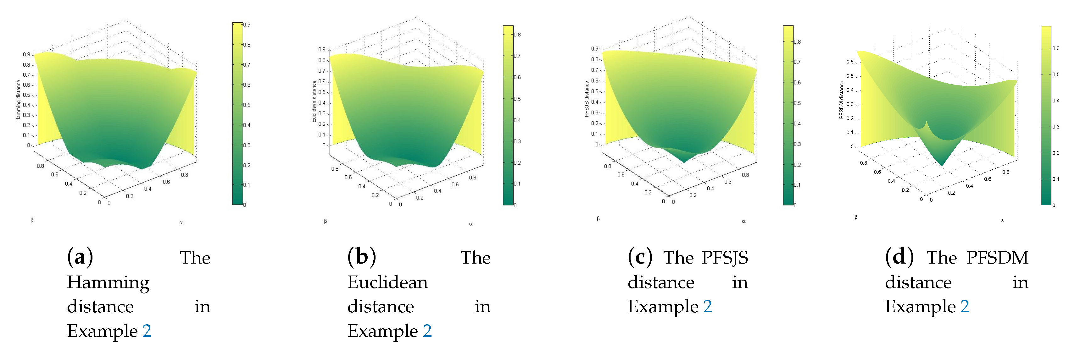
Example 2.

Assume two PFSs $M=\langle x,0.3,0.4\rangle$ and $N=\langle x,\alpha ,\beta \rangle$.

The Hamming distance [55] $D_{Hm}(M,N)$, Euclidean distance [55]$D_E(M,N)$, PFSJS distance [57]$D_{Xiao}(M,N)$, and PFSDM distance $D_{mp}(M,N)$ are displayed in Figure 2a–d.

We can know from the observation that Figure 2a–c have similar trends, but the PFSDM distance is different in Figure 2d. It resembles an inverted cone centered on the point $\langle \alpha =0.3,\beta =0.4\rangle$ because it has a more uniform trend as α and β change. Suppose four PFSs $A1$, $A2$, $B1$, $B2$ as follows:

• $A1=\langle x,A{1}_Y\left(x\right),A{1}_N\left(x\right)\rangle =\langle x,0.1200,0.1600\rangle$,
• $A2=\langle x,A{2}_Y\left(x\right),A{2}_N\left(x\right)\rangle =\langle x,0.1380,0.1840\rangle$,
• $B1=\langle x,B{1}_Y\left(x\right),B{1}_N\left(x\right)\rangle =\langle x,0.5220,0.6960\rangle$,
• $B2=\langle x,B{2}_Y\left(x\right),B{2}_N\left(x\right)\rangle =\langle x,0.5400,0.7200\rangle$.

After calculation, we know that

$$A{2}_Y\left(x\right)-A{1}_Y\left(x\right)=B{2}_Y\left(x\right)-B{1}_Y\left(x\right)=0.0180A{2}_N\left(x\right)-A{1}_N\left(x\right)=B{2}_N\left(x\right)-B{1}_N\left(x\right)=0.0240.$$

To verify that PFSDM distance changes more evenly, the Hamming distance [55] $D_{Hm}(A1,A2)$ and $D_{Hm}(B1,B2)$, Euclidean distance [55]$D_E(A1,A2)$ and $D_E(B1,B2)$, PFSJS distance [57]$D_{Xiao}(A1,A2)$ and $D_{Xiao}(B1,B2)$, PFSDM distance $D_{mp}(A1,A2)$, and $D_{mp}(B1,B2)$ are calculated and results are obtained as follows:

• $D_{Hm}(A1,A2)=0.0129$$D_{Hm}(B1,B2)=0.0531$${\alpha }_{Hm}=D_{Hm}(B1,B2)/D_{Hm}(A1,A2)=4.1163$,
• $D_E(A1,A2)=0.0113$$D_E(B1,B2)=0.0466$${\alpha }_E=D_E(B1,B2)/D_E(A1,A2)=4.1163$,
• $D_{Xiao}(A1,A2)=0.0287$$D_{Xiao}(B1,B2)=0.0256$${\alpha }_{Xiao}=D_{Xiao}(B1,B2)/D_{Xiao}(A1,A2)=2.1021$,
• $D_{mp}(A1,A2)=0.0261$$D_{mp}(B1,B2)=0.0548$${\alpha }_{mp}=D_{mp}(B1,B2)/D_{mp}(A1,A2)=0.8915$.

In the situation of membership degree and non-membership degree changing equally, we can clearly find that the ratio of distance changes α is different, and the PFSDM distance’s ${\alpha }_{mp}$ is closest to 1 among them, which demonstrate that its variation trend is more even than others when membership and non-membership change the same.

The previous examples demonstrate the feasibility of PFSDM distance through numerical analysis. It is well known that pattern recognition is one of the important applications of distance measure. Paul [84] modifies Zhang and Xu’s distance measure of PFSs and applies them to pattern recognition. In the next example, the proposed method is applied {to pattern recognition to prove its rationality.

Example 3.

Suppose a limited universe of discourse $X=\{x_1,x_2,\cdots ,x_{10}\}$, and $A_i(i=1,2,3,4)$ represent four materials of building respectively, and B is an unknown material. Their PFSs are given in

Table 3. The Pythagorean fuzzy sets of building materials in Example 3.

PFS	${\mathit{x}}_1$	${\mathit{x}}_2$	${\mathit{x}}_3$	${\mathit{x}}_4$	${\mathit{x}}_5$
$A_1\left(x\right)$	$\langle x,0.173,0.524\rangle$	$\langle x,0.102,0.818\rangle$	$\langle x,0.530,0.326\rangle$	$\langle x,0.965,0.008\rangle$	$\langle x,0.420,0.351\rangle$
$A_2\left(x\right)$	$\langle x,0.510,0.365\rangle$	$\langle x,0.627,0.125\rangle$	$\langle x,1.000,0.000\rangle$	$\langle x,0.125,0.648\rangle$	$\langle x,0.026,0.823\rangle$
$A_3\left(x\right)$	$\langle x,0.495,0.387\rangle$	$\langle x,0.603,0.298\rangle$	$\langle x,0.987,0.006\rangle$	$\langle x,0.073,0.849\rangle$	$\langle x,0.037,0.923\rangle$
$A_4\left(x\right)$	$\langle x,1.000,0.000\rangle$	$\langle x,1.000,0.000\rangle$	$\langle x,0.857,0.123\rangle$	$\langle x,0.734,0.158\rangle$	$\langle x,0.021,0.896\rangle$
$B_1\left(x\right)$	$\langle x,0.978,0.003\rangle$	$\langle x,0.980,0.012\rangle$	$\langle x,0.798,0.132\rangle$	$\langle x,0.693,0.213\rangle$	$\langle x,0.051,0.876\rangle$
PFS	${\mathit{x}}_{\mathbf{6}}$	${\mathit{x}}_{\mathbf{7}}$	${\mathit{x}}_{\mathbf{8}}$	${\mathit{x}}_{\mathbf{9}}$	${\mathit{x}}_{\mathbf{10}}$
$A_1\left(x\right)$	$\langle x,0.008,0.956\rangle$	$\langle x,0.331,0.512\rangle$	$\langle x,1.000,0.000\rangle$	$\langle x,0.215,0.625\rangle$	$\langle x,0.432,0.534\rangle$
$A_2\left(x\right)$	$\langle x,0.732,0.153\rangle$	$\langle x,0.556,0.303\rangle$	$\langle x,0.650,0.267\rangle$	$\langle x,1.000,0.000\rangle$	$\langle x,0.145,0.762\rangle$
$A_3\left(x\right)$	$\langle x,0.690,0.268\rangle$	$\langle x,0.147,0.812\rangle$	$\langle x,0.213,0.653\rangle$	$\langle x,0.501,0.284\rangle$	$\langle x,1.000,0.000\rangle$
$A_4\left(x\right)$	$\langle x,0.076,0.912\rangle$	$\langle x,0.152,0.712\rangle$	$\langle x,0.113,0.756\rangle$	$\langle x,0.489,0.389\rangle$	$\langle x,1.000,0.000\rangle$
$B_1\left(x\right)$	$\langle x,0.123,0.756\rangle$	$\langle x,0.152,0.721\rangle$	$\langle x,0.113,0.732\rangle$	$\langle x,0.494,0.368\rangle$	$\langle x,0.987,0.000\rangle$

, and we need to recognize the type of B in A by finding the smallest distance $D_{(}{A}_i,B)$ from them. The results of Paul’s method and proposed method, PFSDM distance, are given in

Table 4. The results generated by two methods in Example 3.

$\mathit{Distance}$	$\mathit{D}({\mathit{A}}_1,\mathit{B})$	$\mathit{D}({\mathit{A}}_2,\mathit{B})$	$\mathit{D}({\mathit{A}}_3,\mathit{B})$	$\mathit{D}({\mathit{A}}_4,\mathit{B})$
$Pau{l}^{\prime }smethod$	$0.5970$	$0.5340$	$0.3240$	$\mathbf{0.0740}$
$Proposedmethod$	$0.5296$	$0.5169$	$0.2927$	$\mathbf{0.0486}$

:

In the process of calculation, we use a negligible number such as ${10}^{-8}$ to replace the zero, which is a good method to avoid having a zero denominator. The smallest PFSDM distance of them is $D_{mp}(A_4,B)$, so the material B belongs to $A_4$, which is identical to the result of Paul’s modified method. Hence, PFSDM distance is capable of achieving the desired effect when applied to real-life problems.

In this section, the PFSDM distance for measuring the divergence of PFSs is proposed. Some numerical examples are used to prove its properties and compared with other existing methods. The PFSDM distance has been proven that it not only is rational and practical but has more powerful resolution and a more uniform trend as well, which is because the proposed method combines the properties of BPA handling uncertainty and divergence’s character distinguishing similar data.

4. Application in Medical Diagnosis

In this section, a modified algorithm for medical diagnosis is designed, which is improved based on Xiao’s algorithm [57]. The new algorithm utilizes the PFSDM distance and obtains excellent results in application.

Problem statement: Suppose a limited universe of discourse $X=\{x_1,x_2,x_3,\cdots ,x_n\}$, and the $x_i$ represent the symptoms of diseases and patients. Assume existing m number of patients listed as $P=\{P_1,P_2,\cdots ,P_m\}$ and o number of diseases listed as $D=\{D_1,D_2,\cdots ,D_o\}$. The symptoms of diseases and patients represented by Pythagorean fuzzy sets are as follows:

$$D_i=\{\langle x_1,D_Y^i\left(x_1\right),D_N^i\left(x_1\right)\rangle ,\langle x_2,D_Y^i\left(x_2\right),D_N^i\left(x_2\right)\rangle ,\cdots ,\langle x_n,D_Y^i\left(x_n\right),D_N^i\left(x_n\right)\rangle \}(1\le i\le o),$$

$$P_j=\{\langle x_1,P_Y^j\left(x_1\right),P_N^j\left(x_1\right)\rangle ,\langle x_2,P_Y^j\left(x_2\right),P_N^j\left(x_2\right)\rangle ,\cdots ,\langle x_n,P_Y^j\left(x_n\right),P_N^j\left(x_n\right)\rangle \}(1\le j\le m).$$

We need to utilize the distance measure to recognize which diseases the patients contract.

Step1

For every symptom, calculate the PFSDM distance $D_{mpt}^i(D_t^i,P_t^j)$ in terms of Equation (20) between $D_t^i$ and $P_t^j$, where $(1\le t\ge n)$.

Step2

Calculate the weight of every symptom in medical diagnosis:

${\omega }_t=\frac{D_{mpt}^i(D_t^i,P_t^j)}{{\sum }_1^n{D}_{mpt}^i(D_t^i,P_t^j)}$.

Step3

Diagnose the symptoms of the patient and the symptoms of the disease.

Calculate the weighted average PFSDM distance ${\overline{D}}_{mp}(D_i,P_j)={\sum }_{t=1}^n{\omega }_t{D}_{mpt}^i(D_t^i,P_t^j)$.

Step4

For each weighted average PFSDM distance, the patients $P_j$ can be classified to diseases $D_i$, in which $\xi =mi{n}_{1\le i\le m}\left\{{\overline{D}}_{mp}(D_i,P_j)\right\}$, $P_j\to D_{\xi }$.

When the specific symptoms of the patient conflict with the symptoms of the disease, the proposed algorithm considers that the conflicted symptoms are paid more attention in the medical diagnosis. If all symptoms are diagnosed with the same weight, abnormal symptoms will be ignored when the symptom base is large. In the later examples, the applications of the proposed algorithm and its comparisons with other existing algorithm are shown.

Example 4.

([85]) Assume there are four patients, $Ram$, $Mari$, $Sugu$, and $Somu$, denoted as $P=\{P_1,P_2,$$P_3,P_4\}$. Five symptoms, $Temperature$, $Headache$, $Stomachpain$, $Cough$, and $Chestpain$, are observed, denoted as $S=\{s_1,s_2,s_3,s_4,s_5\}$. Additionally, five diagnoses, $Viralfever$, $Malaria$, $Typhoid$, $Stomachproblems$, and $Chestproblems$, are defined, represented as $D=\{D_1,D_2,D_3,D_4,D_5\}$. Then, the Pythagorean fuzzy relations $P\to S$ and $D\to S$ are displayed in

Table 5. The symptoms of the patients in Example 4.

$\mathit{Patient}$	${\mathit{s}}_1$	${\mathit{s}}_2$	${\mathit{s}}_3$	${\mathit{s}}_4$	${\mathit{s}}_5$
$P_1$	$\langle s_1,0.90,0.10\rangle$	$\langle s_2,0.70,0.20\rangle$	$\langle s_3,0.20,0.80\rangle$	$\langle s_4,0.70,0.20\rangle$	$\langle s_5,0.20,0.70\rangle$
$P_2$	$\langle s_1,0.00,0.70\rangle$	$\langle s_2,0.40,0.50\rangle$	$\langle s_3,0.60,0.20\rangle$	$\langle s_4,0.20,0.70\rangle$	$\langle s_5,0.10,0.20\rangle$
$P_3$	$\langle s_1,0.70,0.10\rangle$	$\langle s_2,0.70,0.10\rangle$	$\langle s_3,0.00,0.50\rangle$	$\langle s_4,0.10,0.70\rangle$	$\langle s_5,0.00,0.60\rangle$
$P_4$	$\langle s_1,0.50,0.10\rangle$	$\langle s_2,0.40,0.30\rangle$	$\langle s_3,0.40,0.50\rangle$	$\langle s_4,0.80,0.20\rangle$	$\langle s_5,0.30,0.40\rangle$

and

Table 6. The symptoms of the diagnoses in Example 4.

$\mathit{Diagnose}$	${\mathit{s}}_1$	${\mathit{s}}_2$	${\mathit{s}}_3$	${\mathit{s}}_4$	${\mathit{s}}_5$
$D_1$	$\langle s_1,0.30,0.00\rangle$	$\langle s_2,0.30,0.50\rangle$	$\langle s_3,0.20,0.80\rangle$	$\langle s_4,0.70,0.30\rangle$	$\langle s_5,0.20,0.60\rangle$
$D_2$	$\langle s_1,0.00,0.60\rangle$	$\langle s_2,0.20,0.60\rangle$	$\langle s_3,0.00,0.80\rangle$	$\langle s_4,0.50,0.00\rangle$	$\langle s_5,0.10,0.80\rangle$
$D_3$	$\langle s_1,0.20,0.20\rangle$	$\langle s_2,0.50,0.20\rangle$	$\langle s_3,0.10,0.70\rangle$	$\langle s_4,0.20,0.60\rangle$	$\langle s_5,0.20,0.80\rangle$
$D_4$	$\langle s_1,0.20,0.80\rangle$	$\langle s_2,0.10,0.50\rangle$	$\langle s_3,0.70,0.00\rangle$	$\langle s_4,0.10,0.70\rangle$	$\langle s_5,0.20,0.70\rangle$
$D_5$	$\langle s_1,0.20,0.80\rangle$	$\langle s_2,0.00,0.70\rangle$	$\langle s_3,0.20,0.80\rangle$	$\langle s_4,0.10,0.80\rangle$	$\langle s_5,0.80,0.10\rangle$

.

The results diagnosis by the proposed algorithm and Xiao’s method [57] are displayed in

Table 7. The results generated by the Xiao method in Example 4.

$\mathit{Patient}$	${\mathit{D}}_1$	${\mathit{D}}_2$	${\mathit{D}}_3$	${\mathit{D}}_4$	${\mathit{D}}_5$	$\mathit{Classification}$
$P_1$	$\mathbf{0.2583}$	$0.3799$	$0.3512$	$0.5295$	$0.5528$	$D_1:Viralfever$
$P_2$	$0.4348$	$0.4217$	$0.4034$	$\mathbf{0.2394}$	3842	$D_4:Stomachproblems$
$P_3$	$0.3925$	$0.4787$	$\mathbf{0.2681}$	$0.4140$	$0.5166$	$D_3:Typhoid$
$P_4$	$\mathbf{0.2166}$	$0.4133$	$0.3454$	$0.4716$	$0.5382$	$D_1:Viralfever$

and

Table 8. The results generated by the proposed method in Example 4.

$\mathit{Patient}$	${\mathit{D}}_1$	${\mathit{D}}_2$	${\mathit{D}}_3$	${\mathit{D}}_4$	${\mathit{D}}_5$	$\mathit{Classification}$
$P_1$	$\mathbf{0.4064}$	$0.6139$	$0.4984$	$0.7587$	$0.7776$	$D_1:Viralfever$
$P_2$	$0.6001$	$0.5971$	$0.5031$	$\mathbf{0.2703}$	5281	$D_4:Stomachproblems$
$P_3$	$0.4807$	$0.6617$	$\mathbf{0.2890}$	$0.7109$	$0.7285$	$D_3:Typhoid$
$P_4$	$\mathbf{0.2407}$	$0.4824$	$0.4475$	$0.5996$	$0.6271$	$D_1:Viralfever$

. By observing the experimental results of proposed method, it is obvious that the $P_1$ has the least ${\overline{D}}_{mp}$$0.4064$ for $D_1$, $P_2$ has the least ${\overline{D}}_{mp}$$0.2703$ for $D_4$, $P_3$ has the least ${\overline{D}}_{mp}$$0.2890$ for $D_3$, and $P_4$ has the least ${\overline{D}}_{mp}$$0.2470$ for $D_1$; Hence, the conclusions are obvious in Table 8.

As shown in

Table 9. The results generated by other methods in Example 4.

$\mathit{Method}$	${\mathit{P}}_1$	${\mathit{P}}_2$	${\mathit{P}}_3$	${\mathit{P}}_4$
$Xiao.$ [57]	$Viralfever$	$Stomachproblems$	$Typhoid$	$Viralfever$
$SamuelandRajakumar$ [86]	$Viralfever$	$Stomachproblems$	$Typhoid$	$Viralfever$
$Proposedmethod$	$Viralfever$	$Stomachproblems$	$Typhoid$	$Viralfever$

, obviously the proposed method generates the same results as Samuel’s method and Xiao’s method, which can demonstrate that the proposed algorithm is capable of finishing medical diagnosis problems. In addition to doing this, we can find that the proposed method has better resolution than Xiao’s method by observing Table 7 and Table 8.

Example 5.

([2,11,57,87,88,89,90]) Assume four patients exist, namely, $David$, $Tom$, $Kim$, and $Bob$, denoted as $P=\{P_1,P_2,P_3,P_4\}$. Five symptoms are observed, in which they are $Temperature$, $Headache$, $Stomachpain$, $Cough$, and $Chestpain$, denoted as $S=\{s_1,s_2,s_3,s_4,s_5\}$. Additionally, five diagnoses, namely, $ViralFever$, $Malaria$, $Typhoid$, $Stomachproblems$, and $Chestproblems$, are defined, represented as $D=\{D_1,D_2,D_3,D_4,D_5\}$. The numerical values respectively represented the membership and non-membership grade of the Pythagorean fuzzy set. Then, through the evaluation of the proposed distance measurement, the Pythagorean fuzzy sets’ distance of $P\to S$ and the Pythagorean fuzzy sets’ distance of $D\to S$ are displayed in the following

Table 10. The symptoms of the patients in Example 5.

$\mathit{Patient}$	${\mathit{s}}_1$	${\mathit{s}}_2$	${\mathit{s}}_3$	${\mathit{s}}_4$	${\mathit{s}}_5$
$P_1$	$\langle s_1,0.80,0.10\rangle$	$\langle s_2,0.60,0.10\rangle$	$\langle s_3,0.20,0.80\rangle$	$\langle s_4,0.60,0.10\rangle$	$\langle s_5,0.10,0.60\rangle$
$P_2$	$\langle s_1,0.00,0.80\rangle$	$\langle s_2,0.40,0.40\rangle$	$\langle s_3,0.60,0.10\rangle$	$\langle s_4,0.10,0.70\rangle$	$\langle s_5,0.10,0.80\rangle$
$P_3$	$\langle s_1,0.80,0.10\rangle$	$\langle s_2,0.80,0.10\rangle$	$\langle s_3,0.00,0.60\rangle$	$\langle s_4,0.20,0.70\rangle$	$\langle s_5,0.00,0.50\rangle$
$P_4$	$\langle s_1,0.60,0.10\rangle$	$\langle s_2,0.50,0.40\rangle$	$\langle s_3,0.30,0.40\rangle$	$\langle s_4,0.70,0.20\rangle$	$\langle s_5,0.30,0.40\rangle$

and

Table 11. The symptoms of the diagnoses in Example 5.

$\mathit{Diagnose}$	${\mathit{s}}_1$	${\mathit{s}}_2$	${\mathit{s}}_3$	${\mathit{s}}_4$	${\mathit{s}}_5$
$D_1$	$\langle s_1,0.40,0.00\rangle$	$\langle s_2,0.40,0.40\rangle$	$\langle s_3,0.10,0.70\rangle$	$\langle s_4,0.40,0.00\rangle$	$\langle s_5,0.10,0.70\rangle$
$D_2$	$\langle s_1,0.70,0.00\rangle$	$\langle s_2,0.20,0.60\rangle$	$\langle s_3,0.00,0.90\rangle$	$\langle s_4,0.70,0.00\rangle$	$\langle s_5,0.10,0.80\rangle$
$D_3$	$\langle s_1,0.30,0.30\rangle$	$\langle s_2,0.60,0.10\rangle$	$\langle s_3,0.20,0.70\rangle$	$\langle s_4,0.20,0.60\rangle$	$\langle s_5,0.10,0.90\rangle$
$D_4$	$\langle s_1,0.10,0.70\rangle$	$\langle s_2,0.20,0.40\rangle$	$\langle s_3,0.80,0.00\rangle$	$\langle s_4,0.20,0.70\rangle$	$\langle s_5,0.20,0.70\rangle$
$D_5$	$\langle s_1,0.10,0.80\rangle$	$\langle s_2,0.00,0.80\rangle$	$\langle s_3,0.20,0.80\rangle$	$\langle s_4,0.20,0.80\rangle$	$\langle s_5,0.80,0.10\rangle$

.

After calculating the distance by the proposed method and Xiao’s method to measure the data, the results are generated in

Table 12. The results generated by proposed method in Example 5.

$\mathit{Patient}$	${\mathit{D}}_1$	${\mathit{D}}_2$	${\mathit{D}}_3$	${\mathit{D}}_4$	${\mathit{D}}_5$	$\mathit{Classification}$
$P_1$	$\mathbf{0.2895}$	$0.4163$	$0.4924$	$0.7125$	$0.7958$	$D_1:Viralfever$
$P_2$	$0.6809$	$0.7839$	$0.5058$	$\mathbf{0.1523}$	$0.6711$	$D_4:Stomachproblems$
$P_3$	$0.3604$	$0.5940$	$\mathbf{0.3197}$	$0.7264$	$0.7701$	$D_3:Typhoid$
$P_4$	$\mathbf{0.2867}$	$0.3699$	$0.4478$	$0.5839$	$0.3370$	$D_1:Viralfever$

and

Table 13. The results generated by Xiao’s method in Exmple 5.

$\mathit{Patient}$	${\mathit{D}}_1$	${\mathit{D}}_2$	${\mathit{D}}_3$	${\mathit{D}}_4$	${\mathit{D}}_5$	$\mathit{Classification}$
$P_1$	$0.2511$	$\mathbf{0.2457}$	$0.3110$	$0.5191$	$0.5606$	$D_2:Malaria$
$P_2$	$0.3712$	$0.4955$	$0.3389$	$\mathbf{0.1589}$	$0.4264$	$D_4:Stomachproblems$
$P_3$	$0.3314$	$0.4348$	$\mathbf{0.3126}$	$0.4610$	$0.5310$	$D_3:Typhoid$
$P_4$	$\mathbf{0.2543}$	$0.3195$	$0.3953$	$0.4605$	$0.5564$	$D_1:Viralfever$

. The results of $David$ ($P1$) are different because of the data marked red in Table 10 and Table 11. Though the $D2$ is more similar to $P1$ in other data intuitively, it generates a conflicted data in $Headache$ ($s_2$). We use a weighted average to assign weights to symptoms. Hence, when the patient matches most of the symptoms of the disease, but one of the symptoms conflicts, the proposed algorithm will give greater weight to the effect of this symptom on the diagnosis of the disease, which will make the diagnosis of a complex disease with many symptoms more accurate.

By comparing other applied widely methods of medical diagnosis and their results in

Table 14. The results generated by other methods.

$\mathit{Method}$	${\mathit{P}}_1$	${\mathit{P}}_2$	${\mathit{P}}_3$	${\mathit{P}}_4$
$Szmidtetal.$ [88]	$Viralfever$	$Stomachproblems$	$Typhoid$	$Viralfever$
$Weietãl.$ [11]	$Malaria$	$Stomachproblems$	$Typhoid$	$Viralfever$
$Mondaletal.$ [9]	$Malaria$	$Stomachproblems$	$Typhoid$	$Viralfever$
$Ye$ [90]	$Viralfever$	$Stomachproblems$	$Typhoid$	$Viralfever$
$Vlachosetal.$ [89]	$Viralfever$	$Stomachproblems$	$Typhoid$	$Viralfever$
$Deetal.$ [2]	$Malaria$	$Stomachproblems$	$Typhoid$	$Viralfever$
$Xiaoetal.$ [57]	$Malaria$	$Stomachproblems$	$Typhoid$	$Viralfever$
$Proposedmethod$	$Viralfever$	$Stomachproblems$	$Typhoid$	$Viralfever$

, we can find that the diagnosis of $David$ ($P_1$) is controversial and its results in Table 13 are similar between $Viralfever$ ($D_1$) and $Malaria$ ($D_2$). On the contrary, $Viralfever$ ($D_1$) and $Malaria$ ($D_2$) have a bigger difference in Table 12, which means that the new method is quite certain of the result.

From the above two examples, the magnified method’s feasibility and merits have been demonstrated. The feasibility of the new algorithm is illustrated by comparing the results of three methods in Example 4, and it can be intuitively found from Table 7 and Table 8 that the new algorithm has higher resolution. In the second Example 5, more methods were compared in Table 14. The new algorithm uses weighted summation to make the previously disputed results more certain, which proves that it considers that the higher conflicted symptoms play a more important role in the diagnostic process.

5. Conclusions

In this paper, we propose a new divergence measure, called PFSDM distance, based on belief function, and modify the algorithm based on Xiao’s method. The proposed method can produce intuitive results and its feasibility is proven by comparing with the existing method. In addition to this, the new method has more even change trend and better performance when the PFSs have larger hesitancy. In addition, we then apply the new algorithm to medical diagnosis and get the desired effect. The new algorithm has better resolution, which is helpful to ruling thresholds in practical applications. Consequently, the main contributions of this article are as follows:

• A method to express the PFS in the form of BPA is proposed, which is the first time to establish a link between them.
• A new distance measure between PFSs, called the PFSDM distance, based on Jensen–Shannon divergence and belief function, is proposed. Combining the characters of divergence and BPA contributes to more powerful resolution and even more of a change trend than existing methods.
• A modified medical diagnosis algorithm is proposed based on Xiao’s method, which utilized the weighted summation to magnify the resolution of algorithm and increase the influence of conflicted data.
• The new divergence measure and the modified algorithm both have satisfying performance in the applications of pattern recognition and medical diagnosis.

It is well known that medical diagnosis is not a $100\%$ accurate procedure and uncertainty is always present in cases. Though we get a definite result in Example 5 by the proposed algorithm, more cases are supposed to be examined in further research to get a safer result. In future research, we will try to explore more PFSs’ properties by using the belief function in evidence theory further and apply them to more situations such as the multi-criteria decision-making and pattern recognition.

References

- Cao, Z.; Ding, W.; Wang, Y.K.; Hussain, F.K.; Al-Jumaily, A.; Lin, C.T. Effects of Repetitive SSVEPs on EEG Complexity using Multiscale Inherent Fuzzy Entropy. Neurocomputing 2019. [Google Scholar] [CrossRef] [Green Version]
- De, S.K.; Biswas, R.; Roy, A.R. An application of intuitionistic fuzzy sets in medical diagnosis. Fuzzy Sets Syst. 2001, 117, 209–213. [Google Scholar] [CrossRef]
- Cao, Z.; Lin, C.T.; Lai, K.L.; Ko, L.W.; King, J.T.; Liao, K.K.; Fuh, J.L.; Wang, S.J. Extraction of SSVEPs-based Inherent fuzzy entropy using a wearable headband EEG in migraine patients. IEEE Trans. Fuzzy Syst. 2019. [Google Scholar] [CrossRef] [Green Version]
- Ding, W.; Lin, C.T.; Cao, Z. Deep neuro-cognitive co-evolution for fuzzy attribute reduction by quantum leaping PSO with nearest-neighbor memeplexes. IEEE Trans. Cybern. 2018, 49, 2744–2757. [Google Scholar] [CrossRef]
- Xiao, F. EFMCDM: Evidential fuzzy multicriteria decision-making based on belief entropy. IEEE Trans. Fuzzy Syst. 2019. [Google Scholar] [CrossRef]
- Tripathy, B.; Arun, K. A new approach to soft sets, soft multisets and their properties. Int. J. Reason.-Based Intell. Syst. 2015, 7, 244–253. [Google Scholar] [CrossRef]
- Song, Y.; Fu, Q.; Wang, Y.F.; Wang, X. Divergence-based cross entropy and uncertainty measures of Atanassov’s intuitionistic fuzzy sets with their application in decision making. Appl. Soft Comput. 2019, 84, 105703. [Google Scholar] [CrossRef]
- Feng, F.; Liang, M.; Fujita, H.; Yager, R.R.; Liu, X. Lexicographic Orders of Intuitionistic Fuzzy Values and Their Relationships. Mathematics 2019, 7, 166. [Google Scholar] [CrossRef] [Green Version]
- Mondal, K.; Pramanik, S. Intuitionistic fuzzy similarity measure based on tangent function and its application to multi-attribute decision-making. Glob. J. Adv. Res. 2015, 2, 464–471. [Google Scholar]
- Song, Y.; Wang, X.; Zhu, J.; Lei, L. Sensor dynamic reliability evaluation based on evidence theory and intuitionistic fuzzy sets. Appl. Intell. 2018, 48, 3950–3962. [Google Scholar] [CrossRef]
- Wei, C.P.; Wang, P.; Zhang, Y.Z. Entropy, similarity measure of interval-valued intuitionistic fuzzy sets and their applications. Inf. Sci. 2011, 181, 4273–4286. [Google Scholar] [CrossRef]
- Dahooie, J.H.; Zavadskas, E.K.; Abolhasani, M.; Vanaki, A.; Turskis, Z. A Novel Approach for Evaluation of Projects Using an Interval–Valued Fuzzy Additive Ratio Assessment ARAS Method: A Case Study of Oil and Gas Well Drilling Projects. Symmetry 2018, 10, 45. [Google Scholar] [CrossRef] [Green Version]
- Pan, Y.; Zhang, L.; Li, Z.; Ding, L. Improved Fuzzy Bayesian Network-Based Risk Analysis With Interval-Valued Fuzzy Sets and D-S Evidence Theory. IEEE Trans. Fuzzy Syst. 2019. [Google Scholar] [CrossRef]
- Ding, W.; Lin, C.T.; Prasad, M.; Cao, Z.; Wang, J. A layered-coevolution-based attribute-boosted reduction using adaptive quantum-behavior PSO and its consistent segmentation for neonates brain tissue. IEEE Trans. Fuzzy Syst. 2017, 26, 1177–1191. [Google Scholar] [CrossRef] [Green Version]
- Gao, X.; Deng, Y. Quantum Model of Mass Function. Int. J. Intell. Syst. 2020, 35, 267–282. [Google Scholar] [CrossRef]
- Chatterjee, K.; Zavadskas, E.K.; Tamoaitien, J.; Adhikary, K.; Kar, S. A Hybrid MCDM Technique for Risk Management in Construction Projects. Symmetry 2018, 10, 46. [Google Scholar] [CrossRef] [Green Version]
- Cao, Z.; Chuang, C.H.; King, J.K.; Lin, C.T. Multi-channel EEG recordings during a sustained-attention driving task. Sci. Data 2019, 6. [Google Scholar] [CrossRef] [Green Version]
- Palash, D.; Hazarika, G.C. Construction of families of probability boxes and corresponding membership functions at different fractiles. Expert Syst. 2017, 34, e12202. [Google Scholar]
- Talhofer, V.; Hošková-Mayerová, Š.; Hofmann, A. Multi-criteria Analysis. In Quality of Spatial Data in Command and Control System; Springer: Cham, Switzerland, 2019; pp. 39–48. [Google Scholar]
- Su, X.; Li, L.; Qian, H.; Sankaran, M.; Deng, Y. A new rule to combine dependent bodies of evidence. Soft Comput. 2019, 23, 9793–9799. [Google Scholar] [CrossRef]
- Jiang, W. A correlation coefficient for belief functions. Int. J. Approx. Reason. 2018, 103, 94–106. [Google Scholar] [CrossRef] [Green Version]
- Dutta, P. An uncertainty measure and fusion rule for conflict evidences of big data via Dempster–Shafer theory. Int. J. Image Data Fusion 2018, 9, 152–169. [Google Scholar] [CrossRef]
- Fu, C.; Chang, W.; Xue, M.; Yang, S. Multiple criteria group decision-making with belief distributions and distributed preference relations. Eur. J. Oper. Res. 2019, 273, 623–633. [Google Scholar] [CrossRef]
- Tripathy, B.; Mittal, D. Hadoop based uncertain possibilistic kernelized c-means algorithms for image segmentation and a comparative analysis. Appl. Soft Comput. 2016, 46, 886–923. [Google Scholar] [CrossRef]
- Seiti, H.; Hafezalkotob, A.; Najaf, S.E. Developing a novel risk-based MCDM approach based on D numbers and fuzzy information axiom and its applications in preventive maintenance planning. Appl. Soft Comput. 2019. [Google Scholar] [CrossRef]
- Seiti, H.; Hafezalkotob, A.; Martinez, L. R-sets, Comprehensive Fuzzy Sets Risk Modeling for Risk-based Information Fusion and Decision-making. IEEE Trans. Fuzzy Syst. 2019. [Google Scholar] [CrossRef]
- Seiti, H.; Hafezalkotob, A. Developing the R-TOPSIS methodology for risk-based preventive maintenance planning: A case study in rolling mill company. Comput. Ind. Eng. 2019, 128, 622–636. [Google Scholar] [CrossRef]
- Jiang, W.; Cao, Y.; Deng, X. A novel Z-network model based on Bayesian network and Z-number. IEEE Trans. Fuzzy Syst. 2019. [Google Scholar] [CrossRef]
- Kang, B.; Zhang, P.; Gao, Z.; Chhipi-Shrestha, G.; Hewage, K.; Sadiq, R. Environmental assessment under uncertainty using Dempster–Shafer theory and Z-numbers. J. Ambient Intell. Humaniz. Comput. 2019, 1–20. [Google Scholar] [CrossRef]
- Seiti, H.; Hafezalkotob, A.; Fattahi, R. Extending a pessimistic–optimistic fuzzy information axiom based approach considering acceptable risk: Application in the selection of maintenance strategy. Appl. Soft Comput. 2018, 67, 895–909. [Google Scholar] [CrossRef]
- Deng, X.; Jiang, W. Evaluating green supply chain management practices under fuzzy environment: A novel method based on D number theory. Int. J. Fuzzy Syst. 2019, 21, 1389–1402. [Google Scholar] [CrossRef]
- Xiao, F.; Zhang, Z.; Abawajy, J. Workflow scheduling in distributed systems under fuzzy environment. J. Intell. Fuzzy Syst. 2019, 37, 5323–5333. [Google Scholar] [CrossRef]
- Chakraborty, S.; Tripathy, B. Privacy preserving anonymization of social networks using eigenvector centrality approach. Intell. Data Anal. 2016, 20, 543–560. [Google Scholar] [CrossRef]
- Fang, R.; Liao, H.; Yang, J.B.; Xu, D.L. Generalised probabilistic linguistic evidential reasoning approach for multi-criteria decision-making under uncertainty. J. Oper. Res. Soc. 2019, in press. [Google Scholar] [CrossRef]
- Liao, H.; Wu, X. DNMA: A double normalization-based multiple aggregation method for multi-expert multi-criteria decision-making. Omega 2019. [Google Scholar] [CrossRef]
- Feng, F.; Fujita, H.; Ali, M.I.; Yager, R.R.; Liu, X. Another view on generalized intuitionistic fuzzy soft sets and related multiattribute decision-making methods. IEEE Trans. Fuzzy Syst. 2018, 27, 474–488. [Google Scholar] [CrossRef]
- Fei, L. On interval-valued fuzzy decision-making using soft likelihood functions. Int. J. Intell. Syst. 2019, 34, 1631–1652. [Google Scholar] [CrossRef]
- Liao, H.; Mi, X.; Xu, Z. A survey of decision-making methods with probabilistic linguistic information: Bibliometrics, preliminaries, methodologies, applications and future directions. Fuzzy Optim. Decis. Mak. 2019. [Google Scholar] [CrossRef]
- Mardani, A.; Nilashi, M.; Zavadskas, E.K.; Awang, S.R.; Zare, H.; Jamal, N.M. Decision Making Methods Based on Fuzzy Aggregation Operators: Three Decades Review from 1986 to 2017. Int. J. Inf. Technol. Decis. Mak. 2018, 17, 391–466. [Google Scholar] [CrossRef]
- Zhou, D.; Al-Durra, A.; Zhang, K.; Ravey, A.; Gao, F. A robust prognostic indicator for renewable energy technologies: A novel error correction grey prediction model. IEEE Trans. Ind. Electron. 2019, 66, 9312–9325. [Google Scholar] [CrossRef]
- Dutta, P. Modeling of variability and uncertainty in human health risk assessment. MethodsX 2017, 4, 76–85. [Google Scholar] [CrossRef]
- Wu, X.; Liao, H. A consensus-based probabilistic linguistic gained and lost dominance score method. Eur. J. Oper. Res. 2019, 272, 1017–1027. [Google Scholar] [CrossRef]
- Seiti, H.; Hafezalkotob, A.; Najafi, S.; Khalaj, M. A risk-based fuzzy evidential framework for FMEA analysis under uncertainty: An interval-valued DS approach. J. Intell. Fuzzy Syst. 2018, 5, 1–12. [Google Scholar] [CrossRef]
- Liu, B.; Deng, Y. Risk Evaluation in Failure Mode and Effects Analysis Based on D Numbers Theory. Int. J. Comput. Commun. Control 2019, 14, 672–691. [Google Scholar]
- Zadeh, L.A. Fuzzy sets. Inf. Control 1965, 8, 338–353. [Google Scholar] [CrossRef] [Green Version]
- Atanassov, K.T. Intuitionistic fuzzy sets. In Intuitionistic Fuzzy Sets; Springer: Heidelberg, Germany, 1999; pp. 1–137. [Google Scholar]
- Yager, R.R.; Abbasov, A.M. Pythagorean membership grades, complex numbers, and decision-making. Int. J. Intell. Syst. 2013, 28, 436–452. [Google Scholar] [CrossRef]
- Yager, R.R. Pythagorean membership grades in multicriteria decision-making. IEEE Trans. Fuzzy Syst. 2013, 22, 958–965. [Google Scholar] [CrossRef]
- Yager, R.R. Properties and applications of Pythagorean fuzzy sets. In Imprecision and Uncertainty in Information Representation and Processing; Springer: Cham, Switzerland, 2016; pp. 119–136. [Google Scholar]
- Xiao, F. A distance measure for intuitionistic fuzzy sets and its application to pattern classification problems. IEEE Trans. Syst. Man Cybern. Syst. 2019. [Google Scholar] [CrossRef]
- Song, Y.; Wang, X.; Quan, W.; Huang, W. A new approach to construct similarity measure for intuitionistic fuzzy sets. Soft Comput. 2019, 23, 1985–1998. [Google Scholar] [CrossRef]
- Tripathy, B.; Mohanty, R.; Sooraj, T. On intuitionistic fuzzy soft set and its application in group decision-making. In Proceedings of the 2016 International Conference on Emerging Trends in Engineering, Technology and Science (ICETETS), Pudukkottai, India, 24–26 February 2016; pp. 1–5. [Google Scholar]
- Szmidt, E.; Kacprzyk, J. Distances between intuitionistic fuzzy sets. Fuzzy Sets Syst. 2000, 114, 505–518. [Google Scholar] [CrossRef]
- Grzegorzewski, P. Distances between intuitionistic fuzzy sets and/or interval-valued fuzzy sets based on the Hausdorff metric. Fuzzy Sets Syst. 2004, 148, 319–328. [Google Scholar] [CrossRef]
- Chen, T.Y. Remoteness index-based Pythagorean fuzzy VIKOR methods with a generalized distance measure for multiple criteria decision analysis. Inf. Fusion 2018, 41, 129–150. [Google Scholar] [CrossRef]
- Wei, G.; Wei, Y. Similarity measures of Pythagorean fuzzy sets based on the cosine function and their applications. Int. J. Intell. Syst. 2018, 33, 634–652. [Google Scholar] [CrossRef]
- Xiao, F.; Ding, W. Divergence measure of Pythagorean fuzzy sets and its application in medical diagnosis. Appl. Soft Comput. 2019, 79, 254–267. [Google Scholar] [CrossRef]
- Shafer, G. A Mathematical Theory of Evidence; Princeton University Press: Princeton, NJ, USA, 1976; Volume 42. [Google Scholar]
- Dempster, A.P. Upper and lower probability inferences based on a sample from a finite univariate population. Biometrika 1967, 54, 515–528. [Google Scholar] [CrossRef]
- Song, Y.; Deng, Y. Divergence measure of belief function and its application in data fusion. IEEE Access 2019, 7, 107465–107472. [Google Scholar] [CrossRef]
- Kullback, S. Information Theory and Statistics; Courier Corporation: Chelmsford, MA, USA, 1997. [Google Scholar]
- Deng, Y. Deng entropy. Chaos Solitons Fractals 2016, 91, 549–553. [Google Scholar] [CrossRef]
- Zhou, M.; Liu, X.B.; Chen, Y.W.; Qian, X.F.; Yang, J.B.; Wu, J. Assignment of attribute weights with belief distributions for MADM under uncertainties. Knowl.-Based Syst. 2019. [Google Scholar] [CrossRef]
- Deng, X.; Jiang, W. A total uncertainty measure for D numbers based on belief intervals. Int. J. Intell. Syst. 2019, 34, 3302–3316. [Google Scholar] [CrossRef] [Green Version]
- Xiao, F. Generalization of Dempster–Shafer theory: A complex mass function. Appl. Intell. 2019, in press. [Google Scholar]
- Gao, X.; Liu, F.; Pan, L.; Deng, Y.; Tsai, S.B. Uncertainty measure based on Tsallis entropy in evidence theory. Int. J. Intell. Syst. 2019, 34, 3105–3120. [Google Scholar] [CrossRef]
- Wang, H.; Deng, X.; Zhang, Z.; Jiang, W. A New Failure Mode and Effects Analysis Method Based on Dempster–Shafer Theory by Integrating Evidential Network. IEEE Access 2019, 7, 79579–79591. [Google Scholar] [CrossRef]
- Jiang, W.; Zhang, Z.; Deng, X. A Novel Failure Mode and Effects Analysis Method Based on Fuzzy Evidential Reasoning Rules. IEEE Access 2019, 7, 113605–113615. [Google Scholar] [CrossRef]
- Zhang, H.; Deng, Y. Weighted belief function of sensor data fusion in engine fault diagnosis. Soft Comput. 2019. [Google Scholar] [CrossRef]
- Zhou, M.; Liu, X.B.; Chen, Y.W.; Yang, J.B. Evidential reasoning rule for MADM with both weights and reliabilities in group decision-making. Knowl.-Based Syst. 2018, 143, 142–161. [Google Scholar] [CrossRef]
- Liu, Z.; Liu, Y.; Dezert, J.; Cuzzolin, F. Evidence combination based on credal belief redistribution for pattern classification. IEEE Trans. Fuzzy Syst. 2019. [Google Scholar] [CrossRef] [Green Version]
- Zhou, M.; Liu, X.; Yang, J. Evidential reasoning approach for MADM based on incomplete interval value. J. Intell. Fuzzy Syst. 2017, 33, 3707–3721. [Google Scholar] [CrossRef] [Green Version]
- Gao, S.; Deng, Y. An evidential evaluation of nuclear safeguards. Int. J. Distrib. Sens. Netw. 2020, 16. [Google Scholar] [CrossRef] [Green Version]
- Pan, L.; Deng, Y. An association coefficient of belief function and its application in target recognition system. Int. J. Intell. Syst. 2020, 35, 85–104. [Google Scholar] [CrossRef]
- Xu, X.; Xu, H.; Wen, C.; Li, J.; Hou, P.; Zhang, J. A belief rule-based evidence updating method for industrial alarm system design. Control Eng. Pract. 2018, 81, 73–84. [Google Scholar] [CrossRef]
- Xu, X.; Li, S.; Song, X.; Wen, C.; Xu, D. The optimal design of industrial alarm systems based on evidence theory. Control Eng. Pract. 2016, 46, 142–156. [Google Scholar] [CrossRef]
- Li, Y.; Deng, Y. Intuitionistic Evidence Sets. IEEE Access 2019, 7, 106417–106426. [Google Scholar] [CrossRef]
- Luo, Z.; Deng, Y. A matrix method of basic belief assignment’s negation in Dempster–Shafer theory. IEEE Trans. Fuzzy Syst. 2019, 27. [Google Scholar] [CrossRef]
- Jiang, W.; Huang, C.; Deng, X. A new probability transformation method based on a correlation coefficient of belief functions. Int. J. Intell. Syst. 2019, 34, 1337–1347. [Google Scholar] [CrossRef]
- Zhang, W.; Deng, Y. Combining conflicting evidence using the DEMATEL method. Soft Comput. 2019, 23, 8207–8216. [Google Scholar] [CrossRef]
- Wang, Y.; Zhang, K.; Deng, Y. Base belief function: An efficient method of conflict management. J. Ambient Intell. Humaniz. Comput. 2019, 10, 3427–3437. [Google Scholar] [CrossRef]
- Lin, J. Divergence measures based on the Shannon entropy. IEEE Trans. Inf. Theory 1991, 37, 145–151. [Google Scholar] [CrossRef] [Green Version]
- Fei, L.; Deng, Y. Multi-criteria decision-making in Pythagorean fuzzy environment. Appl. Intell. 2019. [Google Scholar] [CrossRef]
- Ejegwa, P.A. Modified Zhang and Xu’s distance measure for Pythagorean fuzzy sets and its application to pattern recognition problems. Neural Comput. Appl. 2019. [Google Scholar] [CrossRef]
- Ngan, R.T.; Ali, M. δ-equality of intuitionistic fuzzy sets: A new proximity measure and applications in medical diagnosis. Appl. Intell. 2018, 48, 499–525. [Google Scholar]
- Samuel, A.E.; Rajakumar, S. Intuitionistic Fuzzy Set with Modal Operators in Medical Diagnosis. Adv. Fuzzy Math. 2017, 12, 167–175. [Google Scholar]
- Peng, X.; Yuan, H.; Yang, Y. Pythagorean fuzzy information measures and their applications. Int. J. Intell. Syst. 2017, 32, 991–1029. [Google Scholar] [CrossRef]
- Szmidt, E.; Kacprzyk, J. Intuitionistic fuzzy sets in intelligent data analysis for medical diagnosis. In International Conference on Computational Science; Springer: Berlin/Heidelberg, Germnay, 2001; pp. 263–271. [Google Scholar]
- Vlachos, I.K.; Sergiadis, G.D. Intuitionistic fuzzy information–applications to pattern recognition. Pattern Recognit. Lett. 2007, 28, 197–206. [Google Scholar] [CrossRef]
- Ye, J. Cosine similarity measures for intuitionistic fuzzy sets and their applications. Math. Comput. Model. 2011, 53, 91–97. [Google Scholar] [CrossRef]
Figure 1.
The results in the proof.
Figure 2.
The results in Example 2.