Fractional Derivatives for Economic Growth Modelling of the Group of Twenty: Application to Prediction


1
Industrial Engineering School, University of Extremadura, 06006 Badajoz, Spain
2
IDMEC, Instituto Superior Técnico, Universidade de Lisboa, 1049-001 Lisbon, Portugal
*
Author to whom correspondence should be addressed.
Mathematics 2020, 8(1), 50; https://0-doi-org.brum.beds.ac.uk/10.3390/math8010050
Submission received: 16 December 2019
/
Revised: 21 December 2019
/
Accepted: 24 December 2019
/
Published: 1 January 2020
(This article belongs to the Special Issue Mathematical Economics: Application of Fractional Calculus)
Abstract
:This paper studies the economic growth of the countries in the Group of Twenty (G20) in the period 1970–2018. It presents dynamic models for the world’s most important national economies, including for the first time several economies which are not highly developed. Additional care has been devoted to the number of years needed for an accurate short-term prediction of future outputs. Integer order and fractional order differential equation models were obtained from the data. Their output is the gross domestic product (GDP) of a G20 country. Models are multi-input; GDP is found from all or some of the following variables: country’s land area, arable land, population, school attendance, gross capital formation (GCF), exports of goods and services, general government final consumption expenditure (GGFCE), and broad money (M3). Results confirm the better performance of fractional models. This has been established employing several summary statistics. Fractional models do not require increasing the number of parameters, neither do they sacrifice the ability to predict GDP evolution in the short-term. It was found that data over 15 years allows building a model with a satisfactory prediction of the evolution of the GDP.
1. Introduction
In this paper, models of economic growth are developed. The economies considered are those of the countries members of the Group of Twenty (G20). The period under consideration consists of the years from 1970 until 2018. The gross domestic product (GDP) is obtained as the output of a dynamic system with eight input variables. The best models found employ derivatives of fractional order. These models are compared with alternative versions with integer order derivatives only. The comparison employs several statistical tools, commonly used to assess the quality of a model to predict future outputs. In this manner, the ability of predicting the evolution of the GDP in the short-term is demonstrated. This paper comes in the sequence of similar models obtained for Portugal, Spain [1], France, Italy [2], all the EU member-states [3], the Group of Seven [4], and China [5]. The success of fractional order models for this purpose has been justified as consistent with the mechanisms of economic growth, and is supported by the results.
Of the countries mentioned above, only China is not a highly developed country. Hence, this paper has, for the first time, long term fractional order economic growth models for several countries which are not highly developed, contributing to show that such models are suitable also for this particular case. It also includes a study of the best number of years included in each model to optimise results.
The remainder of this paper is organised in the following manner. Section 2 describes the G20 and presents a short state-of-the-art. Section 3 explains the methodology followed for economic growth modelling of the G20. Section 4 gives and discusses the results obtained. The main conclusions of this paper are drawn in Section 5.
2. Preliminaries
2.1. The G20
The G20 is a group of 19 countries and one international institution (the European Union), that together account for over of the world’s GDP. Membership comprises all the members of the G7, which are the seven wealthiest advanced countries in the world (the European Union being a permanent invitee, though not an eighth member). Other economies, which are not developed economies (according to the criteria either of the United Nations or of the World Bank), play an important role in the world economic and political scenes because of their size, or at least of their regional importance. For this reason, the G7 conceived an extended international forum comprising such countries, which became the G20. Membership was established by invitation upon foundation of the G20 in 1999. Several summits have taken place every year since then. The most visible get together the heads of state or of the heads of government of the members. Others take place at ministerial level, or further business and trade partnerships.
The G20 members are, in alphabetical order: Argentina (ARG), Australia (AUS), Brazil (BRA), Canada (CAN), China (CHI), the European Union (EUU), France (FRA), Germany (DEU), India (IND), Indonesia (IDN), Italy (ITA), Japan (JPN), Mexico (MEX), Russian Federation (RUS), Saudi Arabia (SAU), South Africa (ZAF), South Korea (KOR), Turkey (TUR), the United Kingdom (GBR), and the United States of America (USA). Notice that France, Germany, Italy and the United Kingdom are also member states of the European Union, and are thus represented both directly and indirectly at meetings. (As of writing, the United Kingdom is about to leave European Union membership, and thus to become only directly represented).
The final year for which data is available is 2018. While the G20 exists since 1999 only, it was decided to extend the analysis further back to 1970. There are two reasons for this. First, data for less than 20 years might suffice to establish some models, but not to validate them, verify their performance over some extended period of time, or test their prediction abilities. Second, the period since 1970 is one for which data is easily found for nearly all countries in the G20. Still, for four members, viz. China, Russia, Saudi Arabia and Turkey, it was impossible to find data for this entire period. (This is not surprising for Russia given that it was part of the Union of Soviet Socialist Republics until 1991. In the other cases poor statistics may be due precisely to the lack of economic development). Restricting the period so that there should be data for all countries would result in too short a period, as mentioned above. Thus, only the remaining sixteen members of the G20 will be considered below. Despite this fact, we will refer to those as the G20.
2.2. Fractional Calculus in Economic Modelling
Several financial and economic models of fractional order have been developed. A current review can be found in [6]. An economic interpretation of fractional derivatives is given in [7]. A review of methods for financial models is given in [4]. The particular case of economic growth was addressed using fractional state-spaces [8,9,10,11], variable order derivatives [12], and pseudo-phase plane and state space analysis [13,14]; the effect of memory obtained with fractional derivatives was studied in [15,16]; fractional diffusion models were used for economic crises [17] and financial markets [18,19].
3. Methodology
This section describes the methodology followed in this paper for economic growth modelling of the G20.
3.1. GDP Models
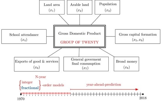
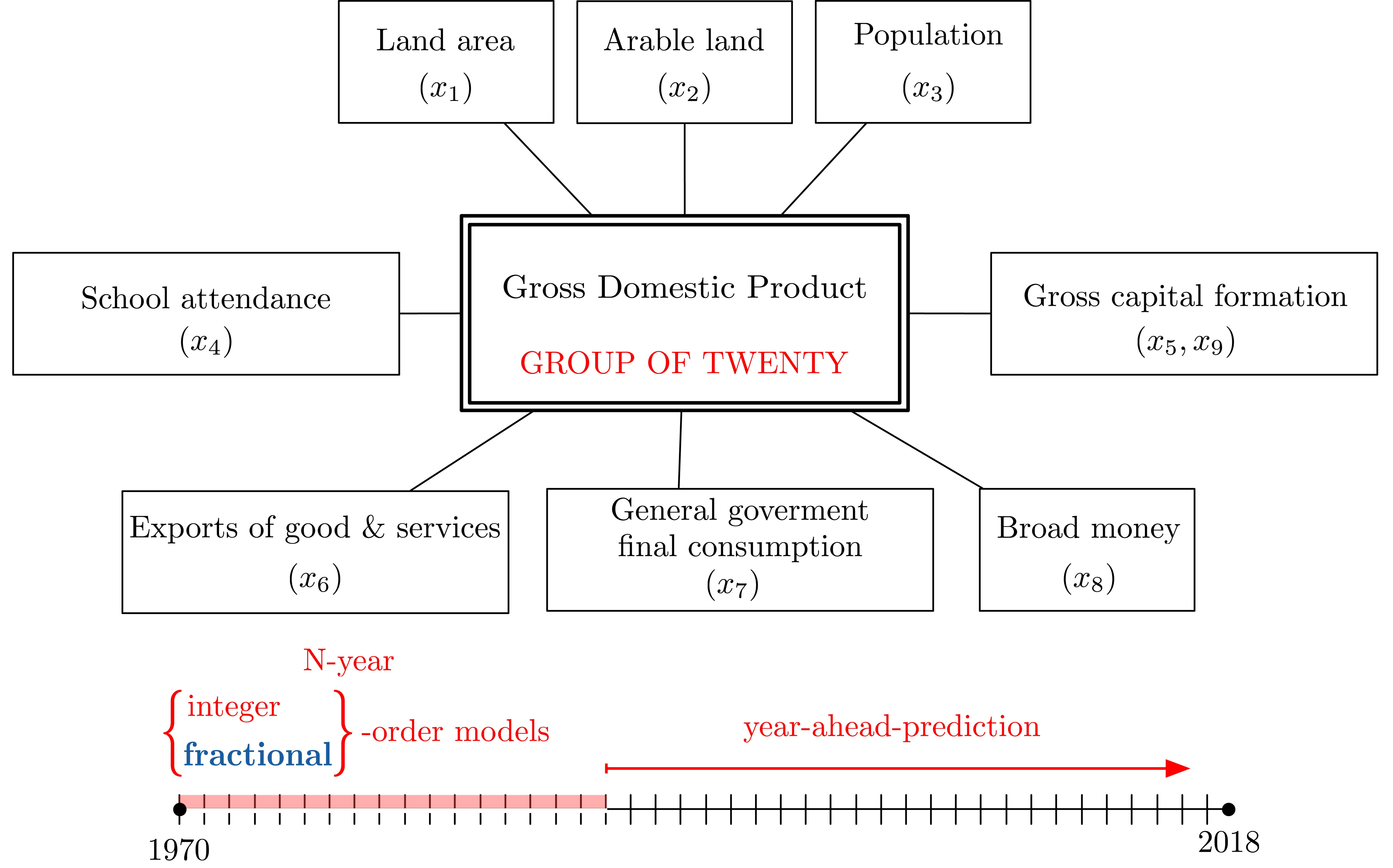
The models presented below rely on the following assumption: the evolution of the GDP is a result of variables of two types. Variables of the first type reflect available resources; variables of the second type reflect impacts on the economy. Consequently, the first model structure conceived for the GDP is a linear integer order differential equation, which is, for each country of the G20, given by:
Variables are as follows:
- : GDP, in 2010 US$;
- : weights, constant in time, for each of the input variables ;
- : first year considered—1970 in this case;
- : inputs of the model, viz.:
- : land area, in km2—measures the natural resources available;
- : arable land, in km2—measures of the quality of the natural resources;
- : population—measures the human resources available;
- : school attendance, in years—measures the quality of human resources;
- : gross capital formation (GCF), in 2010 US$—measures manufactured resources (the model considers the accumulated manufactured resources);
- : exports of goods and services, in 2010 US$—measures external impacts on the economy;
- : general government final consumption expenditure (GGFCE), in 2010 US$—measures budgetary impacts on the economy;
- : broad money (M3), in 2010 US$—measures monetary impacts on the economy (the model considers the variation of monetary impacts);
- : variation of , in 2010 US$—the variation of GCF measures the impact of investment on the economy.
Keynesian models for the dynamics of economies usually consider as inputs variables that have short-term impacts in the economy. Growth accounting usually favors a more long-term approach. (See examples in [20,21,22], and the discussion in [23] about the factors economic growth depends upon). The variables above combine both. Notice that, to make the role of GCF clearer, since it appears twice in the model with different roles, two different variables ( and ) are used to denote it.
As explained below in Section 4.1, not all variables in (1) have the same importance for the accuracy of the model. Their relative importance was found for each country for the whole time period. In this manner simpler models could be obtained. In particular, a second integer order model, with five variables only, was taken as an alternative:
Impacts on the economy have effects that are felt for an extended period of time. Of course, this effect wanes away. Such a behavior can be modelled with fractional derivatives, since fractional derivatives are operators with memory [15,24]. In other words, the fractional derivative of a function is not a local operator, but its value depends on past values of the function. Depending on the particular order employed, this memory of past values can correspond to weights of the said past values that vanish for older time instants. This is the reason fractional derivatives are used to model phenomena such as distributions corresponding to power laws, long tails in general, or chaotic systems [25].
Hence, a fractional generalization of model (2) was considered. Rather than using more variables, and thus recovering model (1), the variables of model (2) representing impacts, and only those, are affected with a fractional derivative. Such variables are , and , so the considered model was:
The sign of the differentiation orders , and can be positive or negative. This type of generalization has already been successfully used in our works [1,2,3,4].
Notice that the resulting fractional model has eight parameters. This is one parameter less than the number of variables of the original integer model (1). As the number of variables is similar, the comparison between the performance of the two is fair. The extra parameter of the integer model gives it a slight advantage; consequently, should the performance turn out to be the same, the fractional model will be considered better, since it achieves the same results with one parameter less.
The fractional differentiation operator was numerically implemented following the Caputo definition [24], as . Years are counted from 1970, which thus corresponds to the lower terminal 0. Terms for initial conditions were not included. Consequently, the effects of inputs are considered only from 1970 on. This approximation reduces statistical data needed to develop models and was used in previously published works, where it has provided acceptable results [4].
3.2. Optimizing and Assessing Performance
A fitting procedure implemented in MATLAB was used to find models (1)–(3) for each of the G20 countries. This procedure relies on Nelder-Mead’s simplex search method. MATLAB’s implementation from function fminsearch was used. The objective was the minimization of the mean square error (MSE):
where N is the number of years— in this case—and and are the GDP and the model’s GDP estimate, respectively. Several performance indexes other than the MSE were used from function regstats to further evaluate the quality of the resulting models, viz.:
- The mean absolute deviation (MAD):
- The coefficient of determination ():where is the mean of the GDP.
- The t-values and p-values for each variable.
In Section 4 it will be shown that not all nine variables , , …, and were necessary for every single model given by (1). This was already the case in models for other countries [1,2,3,4]. This result was established in three ways. First, from the t- and p-values for each variable. Second, from performance indexes MAD and , that should not be significantly worst when one or more variables are removed from the model, if they are indeed necessary. Third, from the Akaike information criterion (AIC):
where K is the number of model parameters. The value of the AIC itself does not give information about the quality of a model. But comparing the AIC values of different models does. With such a comparison, it is possible to find out which models have a higher probability be good models for the data. In fact, a lower value of the AIC denotes a higher probability of a model being the best. Assuming that there are M models, this probability of model i being the best can be normalized as the Akaike weight , by:
In this way, models given by (2) and (3) were developed.
3.3. Models Found from Data for Different Numbers of Years
For each of the expressions (1)–(3), four models were obtained. The first uses the data for the entire 1970–2018 period, so as to obtain a long term fit. This method, however, may lead to overfitting. This can be caused by an excessive influence in parameters of data of too many years into the past. Furthermore, it is impossible to assess the capability of this model of economic growth to predict the future evolution of the economy, because there are no additional years of data for testing the prediction ability.
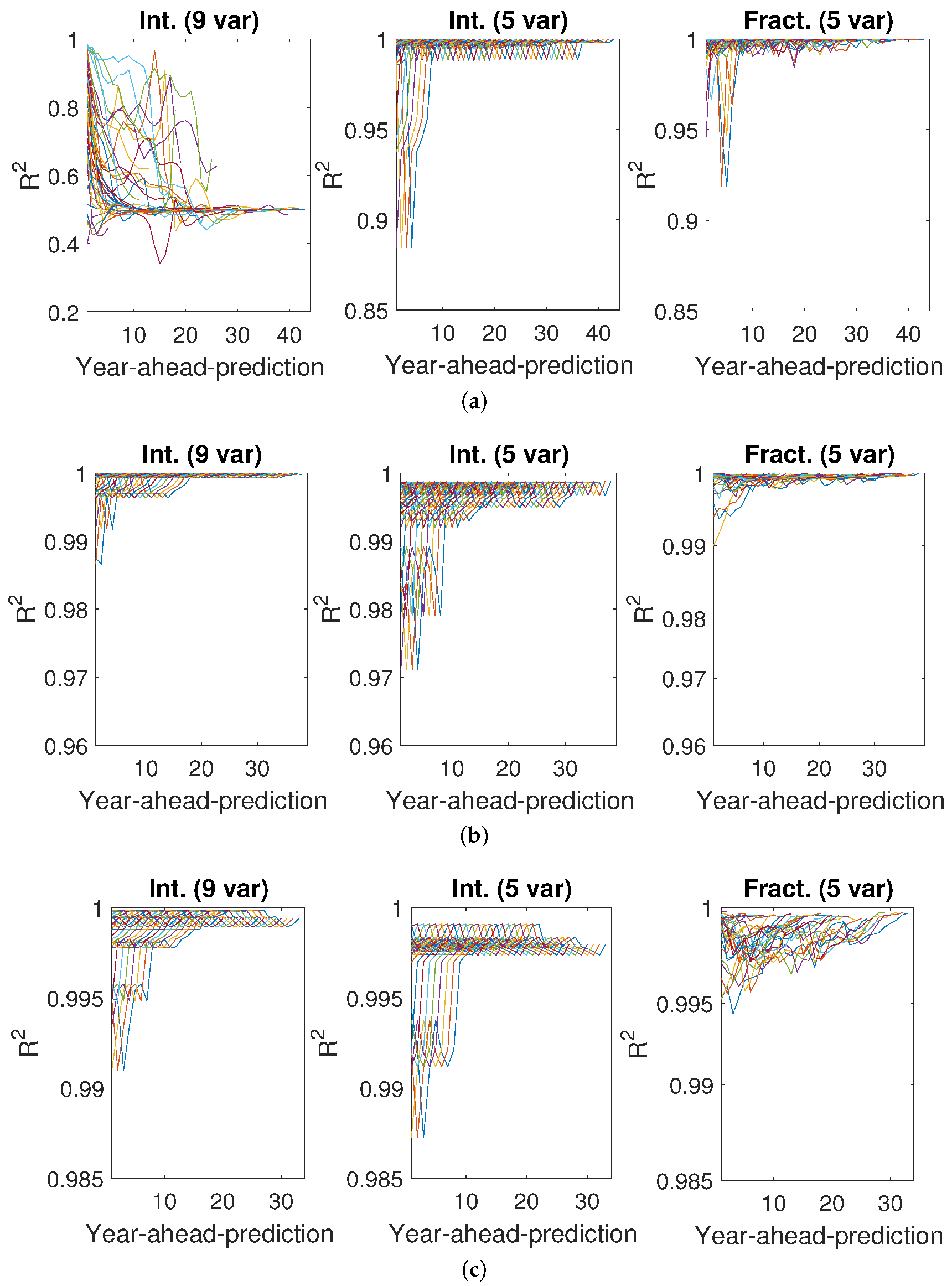
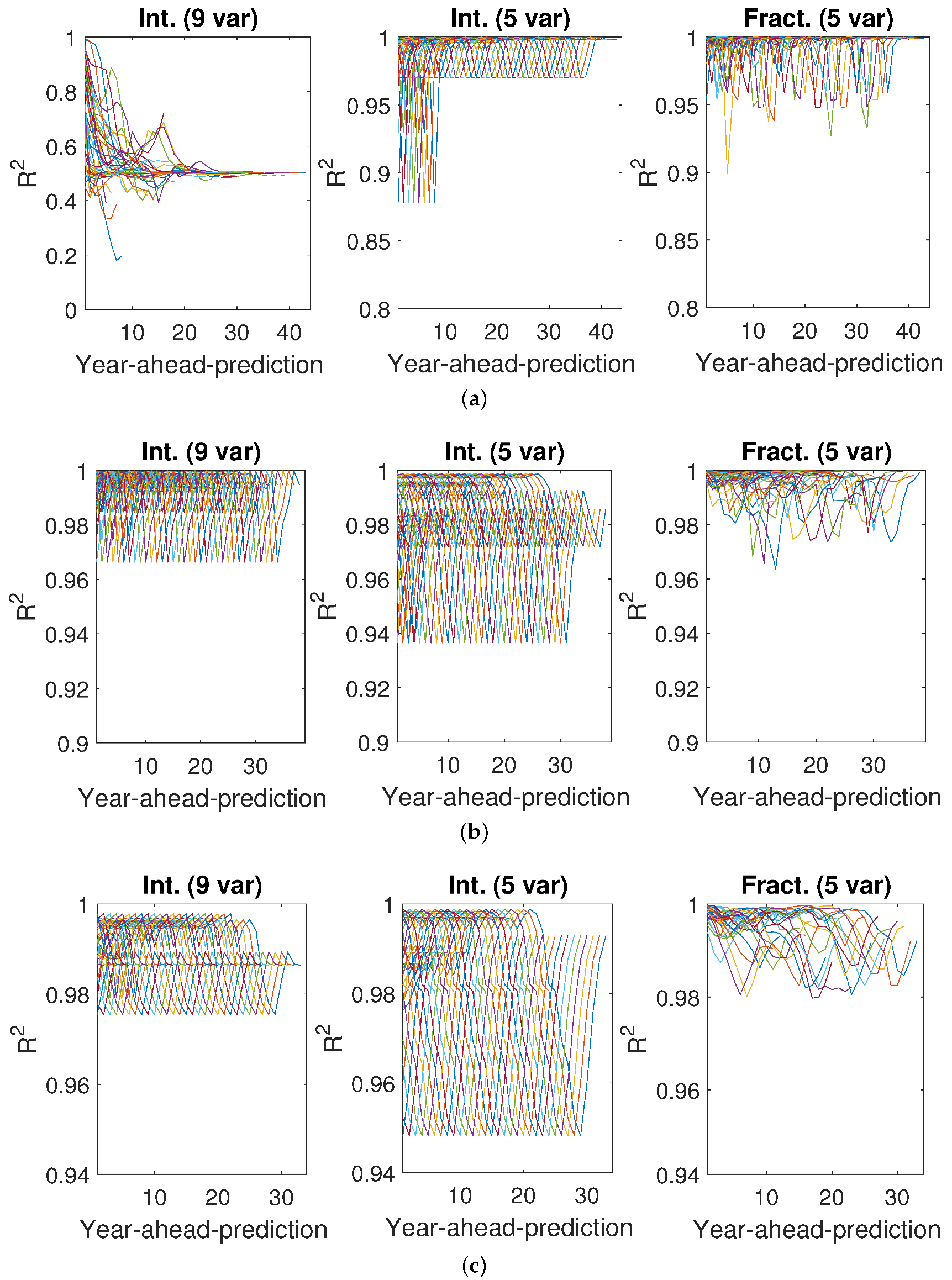
To improve on this, three models for shorter time ranges were obtained. To find out which numbers of years could be reasonable, trend lines were found for the GDP of each country. Both linear and exponential trend lines were obtained; the former provided a better fit for some countries, and the latter for others. Finally, a fast Fourier transform (FFT) was used to obtain, for the different tendencies, the spectral content of the oscillations . This was done in [4] to obtain the best time ranges of models. In the present case, Figure 1 shows the spectral content of these oscillations for all countries, normalized so that every curve peaks at 1. It can be seen that, in the G20, economies do not have similar periods of oscillations around the corresponding tendencies. Within the frequencies where most peaks take place, three reasonable values of time ranges were chosen: periods of 5, 10, and 15 years. In this way, for each country, using (4) as cost function, 34 models were found for , for the periods 1970–1985, 1971–1986, 1972–1987, and so on, such as a moving average; and similarly for (39 models) and (44 models). And this was done separately for models given by (1)–(3). Each of these models can be tested, using for this purpose the data of years in the future. In this manner, it is possible to check how good the model is predicting GDP values which were not used to adjust its parameters. The quality of the prediction was measured with performance indicators MSE, , MAD, AIC, and w for each country.
The GDP of different countries has different orders of magnitude. To make model performance comparison easier, the figures below present the performance index, to show the quality of predictions obtained with each N–year model. The is always in a normalized range, irrespective of the magnitude of the variable under study, which makes it particularly suited for this visual purpose. In this way, all the important characteristics of the different models in relation to the others can be studied.
4. Results
This section presents the models obtained, as well as their performance predicting the GDP of G20 countries. Due to its extension, a full tabulation of results is not included in the paper, but is available in [26]. Data sources are described in Appendix A.
4.1. Models for the 1970–2018 Period
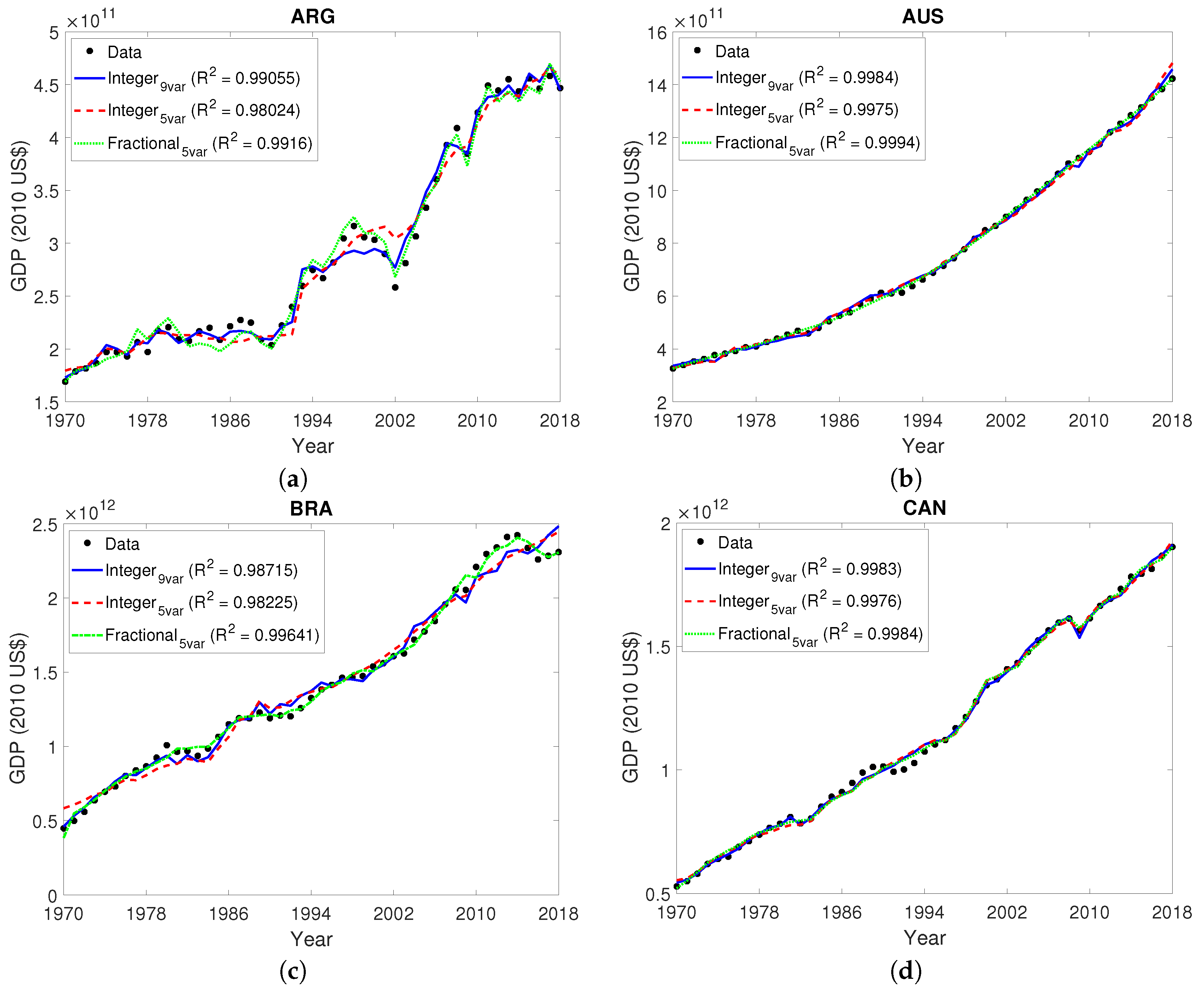
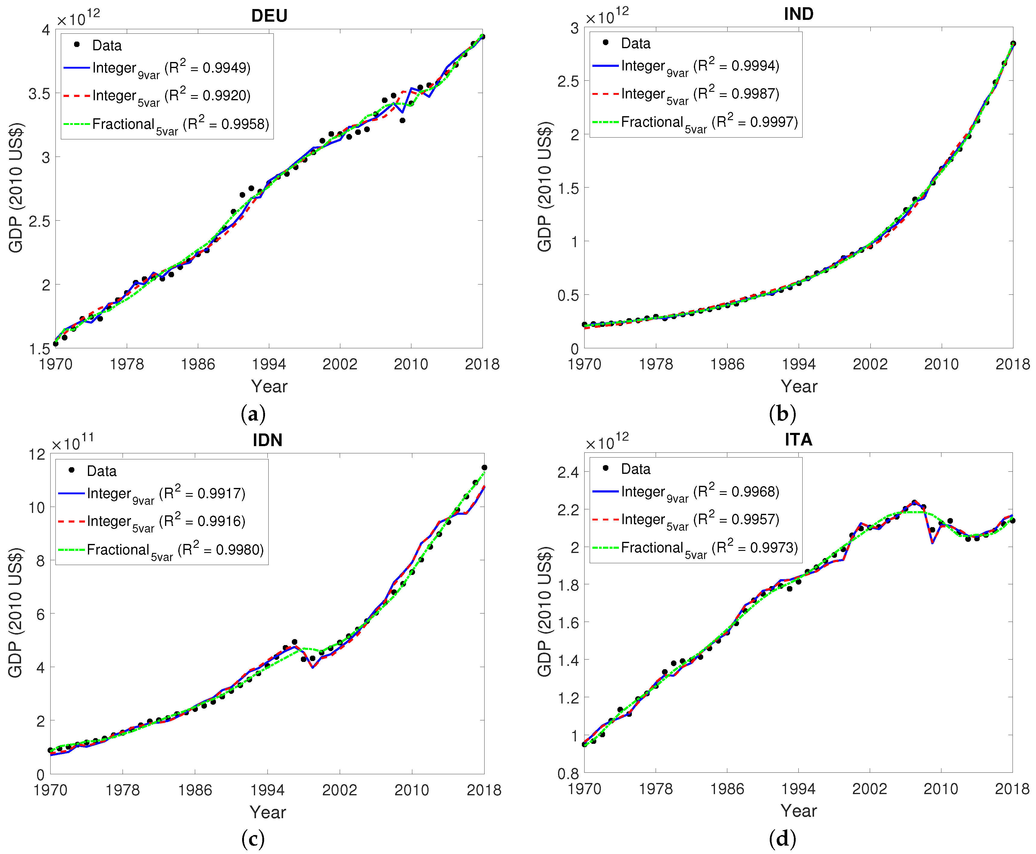
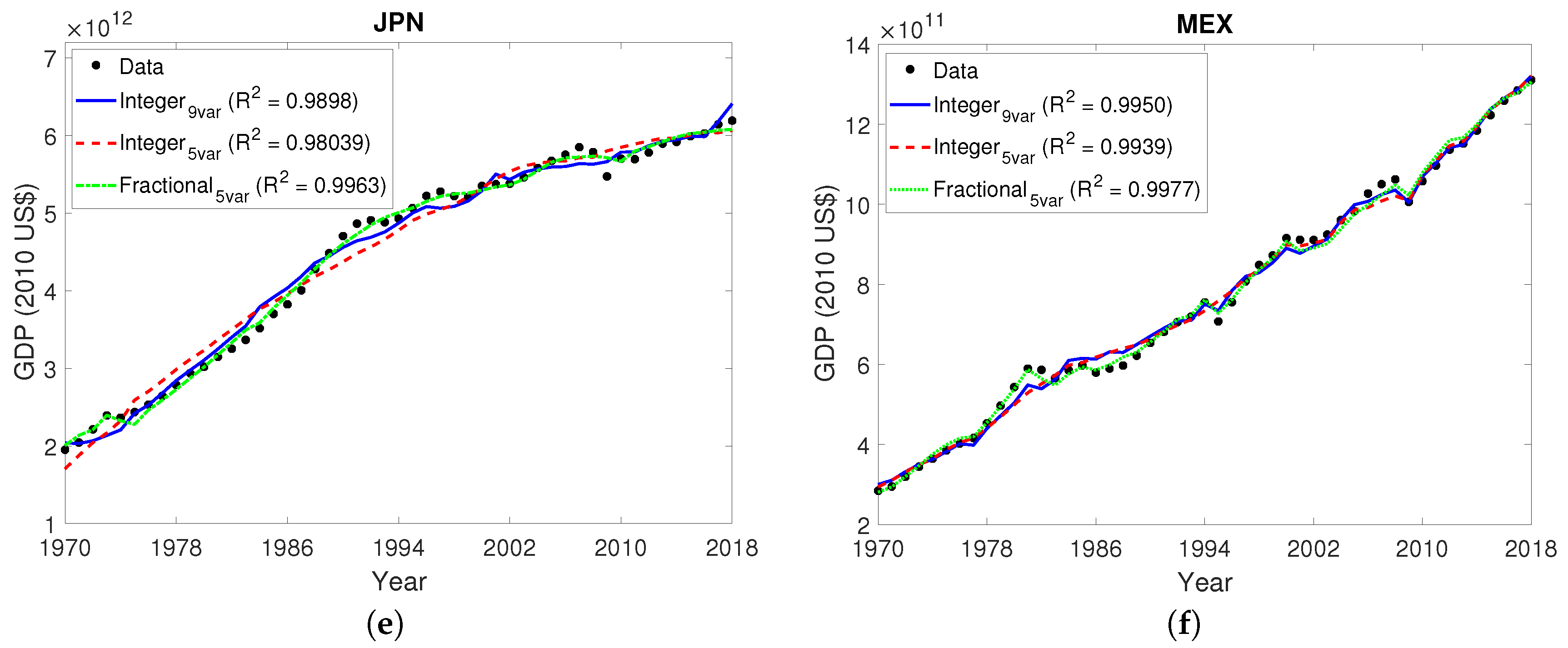
Figure 2, Figure 3 and Figure 4 show the results of the models obtained for each country from data for the entire 1970–2018 period. The performance indices are tabulated in Table 1, Table 2 and Table 3. In those tables, the t-values given in bold are those corresponding to variables which, assuming a 5% significance level, are necessary for the model. This information is also given in Table 4. It turns out that variables important for modelling six or more countries are , , , , and . That is why model (1) could be simplified into model (2), which is in its turn generalized to fractional orders by model (3), only considering , , and to have fractional influence.
As can be observed, the MSE, and MAD allow reaching the same conclusion: the performance of models given by (3) is clearly better than the performance of integer models, in what concerns the quality of the fit during the period used to build each model. This happens for all sixteen countries. The Akaike weight, summarized in the last row of every country, also supports that models (3) are the best of the three for this purpose.
4.2. Models for N–Year Period
Figure 5, Figure 6, Figure 7, Figure 8 and Figure 9 show the performance of integer and fractional models of a group of selected countries (one per continent), namely Australia, the European Union, India, South Africa, and the United States of America, for , 10 and 15 years, predicting the future evolution of the GDP. Showing results for all countries would take too much space; then, results obtained with all models and performance indices can be found in [26] for all countries.
Notice that models obtained with data from periods beginning in the 1970s can be used to predict the GDP for many years until 2018. On the other hand, models developed with data from periods ending in the 21st century can be used to predict the GDP for a few years only. Furthermore, predictions for many years into the future have, as can be expected, a lower performance than those for years close to the end of the data from which the model was got. In fact, the performances in Figure 5, Figure 6, Figure 7, Figure 8 and Figure 9 deteriorate over time, but are quite good at prediction for a short period, and here again fractional models show their better performance, as values do not decrease so significantly.
As far as the number of years for prediction is concerned, it was observed that the smaller the value of N, the better fitting—MSE obtained for every N–year period was really close to zero—but the lower the ability to predict GDP in future: the values of were the smallest of the three cases. This was especially clear for integer model (1). Conversely, the largest the value of N, the lower the value of MSE, but the better the prediction. Notice that the values of for were close to 1, especially for predictions with fractional model (3).
Hence, in order to predict the economic growth of a country of G20 with certainty, it is necessary to consider a relatively large period of years.
5. Conclusions
The models of economic growth, of both integer and fractional order, presented in this paper for countries of the Group of Twenty (G20), from 1970–2018, are satisfactory. The variables chosen to predict variations of gross domestic product (GDP) prove to be suitable to the desired purpose.
It is clear from the results obtained that the performance of fractional models is superior. This statement is qualitatively backed by several indexes. Fractional models do not require an additional number of parameters, neither do they sacrifice the ability to predict the evolution of the GDP in the short-term. As to the number of years needed to build acceptable models, results show that years lead to the best results.
The methodology followed in this paper can be further applied to more countries, and eventually generalised to more variables. Database [27], for instance, includes many time series, usually of good coherence, for all countries, that could be tested in the systematic manner described. The main difficulty is the disparity in the number of years for which time series are available; while for the G20 we could complete the missing values for eight variables, sixteen countries, and forty-nine years, this would likely be very difficult or even impossible if the number of variables, countries or years should be increased. So it would be necessary to improve this methodology in a manner that would cope with missing data and still be able to find, validate and compare models.
Author Contributions
This work involved all coauthors. I.T. wrote the original draft of this manuscript and contributed to the obtaining and the analysis of data and models. E.P. contributed to the obtaining of data and the coding in MATLAB. D.V. supervised all the work and contributed to frequency analysis of the data and the manuscript editing. All authors have read and agreed to the published version of the manuscript.
Funding
This research was supported in part by the Consejería de Economía, Ciencia y Agenda Digital (Junta de Extremadura) under the grant “Ayuda a Grupos de Investigación de Extremadura” (no. GR18159), in part by the European Regional Development Fund “A way to make Europe”, and in part by FCT, through IDMEC, under LAETA, project UID/EMS/50022/2019.
Acknowledgments
The authors would like to thank José Emilio Traver for its help in editing the graphical abstract.
Conflicts of Interest
The authors declare no conflict of interest.
Appendix A. Data Sources
This appendix lists the sources of data used in this paper, which is not tabulated in this paper because of its size. It is available in [28].
- As in [4], variables for the EUU were the sum of the figures for its member states in each year. The only exception was , addressed below.
- The source for the GDP, , , , , , and was [27].
- Variable was available until 2016 only. It was assumed that . For Belgium and Luxemburg, which are member-states of the EUU, there is no data until 2000. Thus, was assumed constant until that year. This approximation corresponds, in the worst case, to an error in of 1.9% for the EUU during those years.
- The source for and for DEU until 1990 was [29]. In the same period, figures for were reduced in the same proportion.
- The source for was [30] until 2010. Figures are available with a 5-year period only, and were interpolated with a third-order spline. The figure for 2010 was extended into the future, using the increase rate of the figures in [31], also interpolated with a third-order spline. However, Figures for the following member-states of the EUU are not found in [30]: Croatia, Estonia, Latvia, Lithuania, Slovenia, Slovak Republic. The source for for these states was [27]. The EUU figure for is a weighted average of the figures for the member states in each year. The weight is the share of each state in .
- Figures for , , and for JPN and USA for 2018 are those of 2017, updated with the yearly growth rate of the index in [32].
- The source for for ARG, AUS, BRA, IDN, IDN, JPN, MEX, ZAF, GBR, and USA was [27].
- The source for for DEU, FRA, ITA and other states of the EUU until 2015 was [33]. Figures were converted to 2010 US$ using the price index in [27]. In the 2016–2018 period, the figure for 2015 was updated with the growth rate in [34,35,36] for DEU, FRA, and ITA, respectively. However, figures for for Luxembourg and Romania in [33] are only available until 2011 and 2013, respectively. The figure for the last year was updated with the growth rate of [27].
References
- Tejado, I.; Valério, D.; Pérez, E.; Valério, N. Fractional calculus in economic growth modelling. The Spanish and Portuguese cases. Int. J. Dyn. Control 2017, 5, 208–222. [Google Scholar] [CrossRef]
- Tejado, I.; Valério, D.; Pérez, E.; Valério, N. Fractional calculus in economic growth modelling: The economies of France and Italy. In Proceedings of the International Conference on Fractional Differentiation and Its Applications, Novi Sad, Serbia, 18–20 July 2016. [Google Scholar]
- Tejado, I.; Pérez, E.; Valério, D. Economic growth in the European Union modelled with fractional derivatives: First results. Bull. Pol. Acad. Sci.-Tech. Sci. 2018, 66, 455–465. [Google Scholar]
- Tejado, I.; Pérez, E.; Valério, D. Fractional calculus in economic growth modelling of the Group of Seven. Fract. Calc. Appl. Anal. 2019, 22, 139–157. [Google Scholar] [CrossRef]
- Ming, H.; Wang, J.R.; Feckan, M. The Application of Fractional Calculus in Chinese Economic Growth Models. Mathematics 2019, 7, 665. [Google Scholar] [CrossRef] [Green Version]
- Tarasov, V.E. On history of mathematical economics: Application of fractional calculus. Mathematics 2019, 7, 509. [Google Scholar] [CrossRef] [Green Version]
- Tarasova, V.V.; Tarasov, V.E. Economic interpretation of fractional derivatives. Progr. Fract. Differ. Appl. 2017, 3, 1–6. [Google Scholar] [CrossRef]
- Hu, Z.; Tu, X. A new discrete economic model involving generalized fractal derivative. Adv. Differ. Equ. 2015, 65. [Google Scholar] [CrossRef]
- Petrás, I.; Podlubny, I. State space description of national economies: The V4 countries. Comput. Stat. Data Anal. 2007, 52, 1223–1233. [Google Scholar] [CrossRef] [Green Version]
- Skovranek, T.; Podlubny, I.; Petrás, I. Modeling of the national economies in state-space: A fractional calculus approach. Econ. Model. 2012, 29, 1322–1327. [Google Scholar] [CrossRef]
- Yue, Y.; He, L.; Liu, G. Modeling and application of a new nonlinear fractional financial model. J. Appl. Math. 2013, 325050. [Google Scholar] [CrossRef]
- Xu, Y.; He, Z. Synchronization of variable-order fractional financial system via active control method. Cent. Eur. J. Phys. 2013, 11, 824–835. [Google Scholar] [CrossRef] [Green Version]
- Tenreiro Machado, J.A.; Mata, M.E. Pseudo phase plane and fractional calculus modeling of western global economic downturn. Commun. Nonlinear Sci. Numer. Simul. 2015, 22, 396–406. [Google Scholar] [CrossRef] [Green Version]
- Tenreiro Machado, J.A.; Mata, M.E.; Lopes, A.M. Fractional state space analysis of economic systems. Entropy 2015, 17, 5402–5421. [Google Scholar] [CrossRef] [Green Version]
- Tarasov, V.E. Long and short memory in economics: Fractional-order difference and differentiation. IRA-Int. J. Manag. Soc. Sci. 2016, 5, 327–334. [Google Scholar] [CrossRef] [Green Version]
- Tarasova, V.V.; Tarasov, V.E. Exact discretization of an economic accelerator and multiplier with memory. Fractal Fract. 2017, 1, 6. [Google Scholar] [CrossRef]
- Caputo, M.; Carcione, J.M.; Botelho, M.A.B. Modeling extreme-event precursors with the fractional diffusion equation. Fract. Calc. Appl. Anal. 2015, 18, 208–222. [Google Scholar] [CrossRef]
- Scalas, E.; Gorenflo, R.; Mainardi, F. Fractional calculus and continuous-time finance. Physica A 2000, 284, 376–384. [Google Scholar] [CrossRef] [Green Version]
- Aguilar, J.-P.; Korbel, J.; Luchko, Y. Applications of the fractional diffusion equation to option pricing and risk calculations. Mathematics 2019, 7, 796. [Google Scholar] [CrossRef] [Green Version]
- Denison, E.F. Why Growth Rates Differ: Postwar Experience in Nine Western Countries; Brookings Institution: Washington, DC, USA, 1967; ISBN 9780815718055. [Google Scholar]
- Lucas, R.E. On the mechanics of economic development. J. Monet. Econ. 1988, 22, 3–42. [Google Scholar] [CrossRef]
- Maddison, A. Explaining the economic performance of nations, 1820–1989. In Convergence of Productivity: Cross-National Studies and Historical Evidence; Baumol, W.J., Nelson, R.R., Wolff, E.N., Eds.; Oxford University Press, Inc.: Oxford, UK, 1994; pp. 20–61. [Google Scholar]
- Van den Berg, H. Economic Growth and Development; World Scientific Publishing Co. Pte. Ltd.: Singapore, 2017; ISBN 978-981-4733-33-5. [Google Scholar]
- Valério, D.; Sá da Costa, J. Introduction to single-input, single-output fractional control. IET Control Theory Appl. 2011, 5, 1033–1057. [Google Scholar] [CrossRef]
- Wang, S.; He, S.; Yousefpour, A.; Jahanshahi, H.; Repnik, R.; Perc, M. Chaos and complexity in a fractional-order financial system with time delays. Chaos Solitons Fractals 2019, 109521. [Google Scholar] [CrossRef]
- Tejado, I.; Pérez, E.; Valério, D. Results for Predictions of the Future Evolution of the GDP for the G20 Group. 2019. Available online: https://github.com/UExtremadura/Economic/blob/master/G20Results_Tejado_et_al2019.rar (accessed on 16 December 2019).
- The World Bank. World Bank Database. 2019. Available online: https://databank.worldbank.org/source/world-development-indicators (accessed on 19 August 2019).
- Tejado, I.; Pérez, E.; Valério, D. Economic Data for the G20 Group. 2019. Available online: https://github.com/UExtremadura/Economic/blob/master/G20Data_Tejado_et_al_Mathematics19.xls (accessed on 16 December 2019).
- West Germany. 2018. Available online: https://en.wikipedia.org/wiki/West_Germany (accessed on 29 August 2018).
- Lee, J.W.; Lee, H. Lee and Lee Long-run Education Dataset, Lee–Lee Database Version 2.2. 2018. Available online: http://www.barrolee.com/Lee_Lee_LRdata_dn.htm (accessed on 29 August 2019).
- Wittgenstein Centre for Demography and Global Human Capital. Wittgenstein Centre Data Explorer Version 2.0. 2018. Available online: http://dataexplorer.wittgensteincentre.org/wcde-v2/ (accessed on 19 August 2019).
- OECD. OECDiLibrary. 2019. Available online: http://0-dx-doi-org.brum.beds.ac.uk/10.1787/1036a2cf-en (accessed on 10 September 2019).
- Federal Reserve Bank of St. Louis. Federal Reserve Economic Data. 2019. Available online: https://fred.stlouisfed.org/ (accessed on 10 September 2019).
- The Global Economy. Economic Indicators for Over 200 Countries: Germany. 2019. Available online: https://www.theglobaleconomy.com/Germany/money_supply/ (accessed on 12 September 2019).
- The Global Economy. Economic Indicators for Over 200 Countries: France. 2019. Available online: https://www.theglobaleconomy.com/France/money_supply/ (accessed on 12 September 2019).
- The Global Economy. Economic Indicators for Over 200 Countries: Italy. 2019. Available online: https://www.theglobaleconomy.com/Italy/money_supply/ (accessed on 12 September 2019).
Figure 1.
Spectral content of the oscillations for all countries, normalized so that every curve has a peak with amplitude 1, where is the GDP, and is a trend line: (a) Linear tendency (b) Exponential tendency (c) The best of the previous two.
Figure 1.
Spectral content of the oscillations for all countries, normalized so that every curve has a peak with amplitude 1, where is the GDP, and is a trend line: (a) Linear tendency (b) Exponential tendency (c) The best of the previous two.

Figure 2.
Results obtained with integer and fractional models for the following members of the G20: (a) Argentina (b) Australia (c) Brazil (d) Canada (e) European Union (f) France. GDP estimations were obtained with integer models (1) and (2) and with fractional model (3). values are given to show the quality of the results of each model. As GDPs have different orders of magnitude, different scales were used in the y-axis for different countries.


Figure 3.
Results obtained with integer and fractional models for the following members of the G20: (a) Germany (b) India (c) Indonesia (d) Italy (e) Japan (f) Mexico. GDP estimations were obtained with integer models (1) and (2) and with fractional model (3). values are given to show the quality of the results of each model. As GDPs have different orders of magnitude, different scales were used in the y-axis for different countries.


Figure 4.
Results obtained with integer and fractional models for the following members of the G20: (a) South Africa (b) Korea (c) United Kingdom (d) United States of America. GDP estimations were obtained with integer models (1) and (2) and with fractional model (3). values are given to show the quality of the results of each model. As GDPs have different orders of magnitude, different scales were used in the y-axis for different countries.

Figure 5.
values of GDP estimates for Australia. Estimates were obtained with models (1) (left), (2) (middle), and (3) (right). The models were obtained with data for different numbers of years: (a) (top) (b) (center) (c) (bottom). The models were used to estimate the GDP for as many years as possible after the period for which they were built. The scale of the y-axis is not the same for all models and all values of N.

Figure 6.
values of GDP estimates for the European Union. Estimates were obtained with models (1) (left), (2) (middle), and (3) (right). The models were obtained with data for different numbers of years: (a) (top) (b) (center) (c) (bottom). The models were used to estimate the GDP for as many years as possible after the period for which they were built. The scale of the y-axis is not the same for all models and all values of N.

Figure 7.
values of GDP estimates for India. Estimates were obtained with models (1) (left), (2) (middle), and (3) (right). The models were obtained with data for different numbers of years: (a) (top) (b) (center) (c) (bottom). The models were used to estimate the GDP for as many years as possible after the period for which they were built. The scale of the y-axis is not the same for all models and all values of N.

Figure 8.
values of GDP estimates for South Africa. Estimates were obtained with models (1) (left), (2) (middle), and (3) (right). The models were obtained with data for different numbers of years: (a) (top) (b) (center) (c) (bottom). The models were used to estimate the GDP for as many years as possible after the period for which they were built. The scale of the y-axis is not the same for all models and all values of N.

Figure 9.
values of GDP estimates for the United States of America. Estimates were obtained with models (1) (left), (2) (middle), and (3) (right). The models were obtained with data for different numbers of years: (a) (top) (b) (center) (c) (bottom). The models were used to estimate the GDP for as many years as possible after the period for which they were built. The scale of the y-axis is not the same for all models and all values of N.


Table 1.
Performance indices of the different models obtained for the G20 members in Figure 2; for an explanation of performance assessment see Section 3.2.
Table 1.
Performance indices of the different models obtained for the G20 members in Figure 2; for an explanation of performance assessment see Section 3.2.
| Argentina | Australia | ||||||
| Index/Statistic | Variable | Integer | Integer | Fractional | Integer | Integer | Fractional |
| (1) | (2) | (3) | (1) | (2) | (3) | ||
| MSE () | 8.355 | 17.475 | 7.423 | 17.608 | 27.232 | 6.235 | |
| 0.9906 | 0.9802 | 0.9916 | 0.9984 | 0.9975 | 0.9994 | ||
| MAD () | 7.761 | 10.101 | 7.614 | 10.208 | 11.986 | 5.467 | |
| t-values | |||||||
| 2.154 | − | − | 1.124 | − | − | ||
| 2.065 | − | − | − | − | |||
| 2.193 | 1.316 | ||||||
| 1.694 | |||||||
| − | − | − | − | ||||
| − | − | − | − | ||||
| AIC () | |||||||
| w (%) | 0 | 0 | 0 | ||||
| Brazil | Canada | ||||||
| Index/Statistic | Variable | Integer | Integer | Fractional | Integer | Integer | Fractional |
| (1) | (2) | (3) | (1) | (2) | (3) | ||
| MSE () | |||||||
| MAD () | |||||||
| t-values | |||||||
| − | − | − | − | ||||
| − | − | − | − | ||||
| − | − | − | − | ||||
| − | − | − | − | ||||
| AIC () | |||||||
| w (%) | 0 | 0 | 0 | ||||
| European Union | France | ||||||
| Index/Statistic | Variable | Integer | Integer | Fractional | Integer | Integer | Fractional |
| (1) | (2) | (3) | (1) | (2) | (3) | ||
| MSE () | |||||||
| MAD () | |||||||
| t-values | |||||||
| − | − | − | − | ||||
| − | − | − | − | ||||
| − | − | − | − | ||||
| − | − | − | − | ||||
| AIC () | |||||||
| w (%) | 0 | 0 | |||||
Table 2.
Performance indices of the different models obtained for the G20 members in Figure 3; for an explanation of performance assessment see Section 3.2.
Table 2.
Performance indices of the different models obtained for the G20 members in Figure 3; for an explanation of performance assessment see Section 3.2.
| Germany | India | ||||||
| Index/Statistic | Variable | Integer | Integer | Fractional | Integer | Integer | Fractional |
| (1) | (2) | (3) | (1) | (2) | (3) | ||
| MSE () | |||||||
| MAD () | |||||||
| t-values | |||||||
| − | − | − | − | ||||
| − | − | − | − | ||||
| − | − | − | − | ||||
| − | − | − | − | ||||
| AIC () | |||||||
| w (%) | 0 | 0 | 0 | 0 | |||
| Indonesia | Italy | ||||||
| Index/Statistic | Variable | Integer | Integer | Fractional | Integer | Integer | Fractional |
| (1) | (2) | (3) | (1) | (2) | (3) | ||
| MSE () | |||||||
| MAD () | |||||||
| t-values | |||||||
| − | − | − | − | ||||
| − | − | − | − | ||||
| − | − | − | − | ||||
| − | − | − | − | ||||
| AIC () | |||||||
| w (%) | 0 | 0 | 0 | ||||
| Japan | Mexico | ||||||
| Index/Statistic | Variable | Integer | Integer | Fractional | Integer | Integer | Fractional |
| (1) | (2) | (3) | (1) | (2) | (3) | ||
| MSE () | |||||||
| MAD () | |||||||
| t-values | |||||||
| − | − | − | − | ||||
| − | − | − | − | ||||
| − | − | − | − | ||||
| − | − | − | − | ||||
| AIC () | |||||||
| w (%) | 0 | 0 | 0 | 0 | |||
Table 3.
Performance indices of the different models obtained for the G20 members in Figure 4; for an explanation of performance assessment see Section 3.2.
Table 3.
Performance indices of the different models obtained for the G20 members in Figure 4; for an explanation of performance assessment see Section 3.2.
| South Africa | Korea | ||||||
| Index/Statistic | Variable | Integer | Integer | Fractional | Integer | Integer | Fractional |
| (1) | (2) | (3) | (1) | (2) | (3) | ||
| MSE () | |||||||
| MAD () | |||||||
| t-values | |||||||
| − | − | − | − | ||||
| − | − | − | − | ||||
| − | − | − | − | ||||
| − | − | − | − | ||||
| AIC () | |||||||
| w (%) | 0 | 0 | 0 | ||||
| United Kingdom | United States of America | ||||||
| Index/Statistic | Variable | Integer | Integer | Fractional | Integer | Integer | Fractional |
| (1) | (2) | (3) | (1) | (2) | (3) | ||
| MSE () | |||||||
| MAD () | |||||||
| t-values | |||||||
| − | − | − | − | ||||
| − | − | − | − | ||||
| − | − | − | − | ||||
| − | − | − | − | ||||
| AIC () | |||||||
| w (%) | 0 | 0 | |||||
Table 4.
Relevance of the independent variables of model (1), from which the GDP depends, for each country; for an explanation of how variable relevance was determined, see Section 4.1.
Table 4.
Relevance of the independent variables of model (1), from which the GDP depends, for each country; for an explanation of how variable relevance was determined, see Section 4.1.
| Argentina | ✓ | ||||||||
| Australia | ✓ | ✓ | ✓ | ||||||
| Brazil | ✓ | ✓ | |||||||
| Canada | ✓ | ✓ | ✓ | ✓ | ✓ | ✓ | |||
| European Union | ✓ | ✓ | ✓ | ||||||
| France | ✓ | ✓ | ✓ | ✓ | ✓ | ✓ | |||
| Germany | ✓ | ✓ | ✓ | ✓ | |||||
| India | ✓ | ✓ | ✓ | ||||||
| Indonesia | ✓ | ✓ | |||||||
| Italy | ✓ | ✓ | ✓ | ✓ | ✓ | ||||
| Japan | ✓ | ✓ | |||||||
| Mexico | ✓ | ✓ | |||||||
| South Africa | ✓ | ✓ | ✓ | ✓ | |||||
| Korea | ✓ | ✓ | |||||||
| United Kingdom | ✓ | ✓ | ✓ | ✓ | |||||
| United States of America | ✓ | ✓ | ✓ | ✓ |
© 2020 by the authors. Licensee MDPI, Basel, Switzerland. This article is an open access article distributed under the terms and conditions of the Creative Commons Attribution (CC BY) license (http://creativecommons.org/licenses/by/4.0/).
Share and Cite
MDPI and ACS Style
Tejado, I.; Pérez, E.; Valério, D. Fractional Derivatives for Economic Growth Modelling of the Group of Twenty: Application to Prediction. Mathematics 2020, 8, 50. https://0-doi-org.brum.beds.ac.uk/10.3390/math8010050
AMA Style
Tejado I, Pérez E, Valério D. Fractional Derivatives for Economic Growth Modelling of the Group of Twenty: Application to Prediction. Mathematics. 2020; 8(1):50. https://0-doi-org.brum.beds.ac.uk/10.3390/math8010050
Chicago/Turabian StyleTejado, Inés, Emiliano Pérez, and Duarte Valério. 2020. "Fractional Derivatives for Economic Growth Modelling of the Group of Twenty: Application to Prediction" Mathematics 8, no. 1: 50. https://0-doi-org.brum.beds.ac.uk/10.3390/math8010050
Note that from the first issue of 2016, this journal uses article numbers instead of page numbers. See further details here.