Asymptotically Normal Estimators of the Gerber-Shiu Function in Classical Insurance Risk Model


School of Insurance, Shandong University of Finance and Economics, Jinan 250014, China
*
Author to whom correspondence should be addressed.
Mathematics 2020, 8(10), 1638; https://0-doi-org.brum.beds.ac.uk/10.3390/math8101638
Submission received: 8 July 2020
/
Revised: 1 August 2020
/
Accepted: 10 August 2020
/
Published: 23 September 2020
(This article belongs to the Special Issue Stochastic Statistics and Modeling)
Abstract
:Nonparametric estimation of the Gerber-Shiu function is a popular topic in insurance risk theory. Zhang and Su (2018) proposed a novel method for estimating the Gerber-Shiu function in classical insurance risk model by Laguerre series expansion based on the claim number and claim sizes of sample. However, whether the estimators are asymptotically normal or not is unknown. In this paper, we give the details to verify the asymptotic normality of these estimators and present some simulation examples to support our result.
1. Introduction
In this paper, we consider the classical risk model
where denotes the initial surplus level and denotes the premium rate. The claim number follows a Poisson process with intensity . denote the claim sizes which are independent and identically distributed random variables with density f and mean . Meanwhile, suppose that and are mutually independent. Let denote ruin time and we set when for all .
Gerber and Shiu [1] considered the expected discounted penalty function about the ruin time , the surplus before ruin time and the deficit at ruin time which is defined
where is a measurable penalty function of and , is the indicator function, is the interest force. In this paper, we verify asymptotically normal estimators of the Gerber-Shiu function when . Many researchers have made remarkable contributions to this model and its generalizations have been made in various risk model. Asmussen and Albercher [2] considered the classical risk model; Gerber and Landry [3], Tsai [4,5] considered the compound Poisson risk model perturbed by diffusion; Yu [6] and Yu et al. [7] investigated the absolute ruin risk model. Zhao and Yin [8] studied the Gerber-Shiu function in Lévy risk model; Xie and Zou [9] and Zhu et al. [10] studied the compound Poisson with delayed claims. The Gerber-Shiu function has also been studied by Yin and Wang [11], Shen et al. [12], Yin and Yuen [13], Cai et al. [14], Deng et al. [15], Dong et al. [16], Wang and Zhang [17], Yu et al. [18], Peng et al. [19] among others.
In all of these mentioned papers, they assumed that the parameter and the claim size density f are known. However, the probability characteristics of the surplus process are usually unknown. Recently, statistical estimation of risk measures based on the observed data information of claim number and claim sizes has become a popular topic, see e.g., Shimizu [20] applied regularized Laplace transform to estimate the Gerber-Shiu function in Lévy risk model; Zhang and Yang [21,22] estimated the ruin probability based on high-frequency observation and low-frequency observation, respectively; Zhang [23] construted an estimator of the Gerber-Shiu by Fourier-Sinc series expansion and Zhang [24] estimated the finite time ruin probability by double Fourier transform. Later, Zhang and Su [25] proposed a new method for estimating the Gerber-Shiu function by Laguerre basis and derived the convergence rate of the estimate. In this paper, we show that the above estimator for the Gerber-Shiu function is asymptotically normal. Asymptotic normality results allow us to establish confidence intervals. For more study on the statistical estimation of risk model, the interested readers are referred to the work of Shimizu and Zhang [26] Yu et al. [27], Peng and Wang [28], Yu et al. [29] and Zhang et al. [30].
The remainder of this paper is organized as follows. We present some preliminaries on Laguerre expansion of Gerber-Shiu function and the estimator of Gerber-Shiu function in Section 2. We give the details to verify the asymptotic normality of these estimators in Section 3. Finally, we present some numerical examples to verify the proposed estimator is asymptotically normal in Section 4.
2. Preliminaries
First, we introduce the following notation:
- , , .
- .
- denotes the Laplace transform of claim size density f,
- denotes the characteristic function of random vector , where t is a random vector in , .
- For , let be the scalar product and be -norm.
- For positive function , let be , where C is a positive constant.
- ⊤ means the transpose of matrix.
- is a zero vector.
- Let be convergence in probability and be convergence in distribution.
- means that for some constant C.
Meanwhile, we need the following conditions, which have also been considered in Zhang and Su [25]:
- Condition 1 The premium rate ;
- Condition 2 Suppose that
- Condition 3 For some , suppose that the penalty function
2.1. Laguerre Expansion of Gerber-Shiu Function
The Laguerre functions are defined by
where . It follows from Abramowitz and Stegun [31] that
- form a complete orthogonal basis over . Then, when , it can be expanded by the Laguerre function:
- are uniformly bounded, i.e.
- , , and for .
According to Gerber and Shiu [1], the Gerber-Shiu function satisfies
where Since by the condition 1, 2 of Zhang and Su [25], can be expressed by Laguerre basis as
where , , . It follows from Zhang and Su [25], we obtain the approximation of the Gerber-Shiu function
where denotes truncation parameter, and . can be expressed as , where and is a lower triangular invertible Toeplitz matrix, whose components are given by
2.2. Coefficient and
By changing the order of integrals, we have
and
where , . Meanwhile, by Condition 3 and are uniformly bounded, we have
and
2.3. Statistical Inference
For insurer, the parameter and the claim size density f are usually unknown. But, they can be obtained by the following data information,
where is the claim number over and are individual claim sizes. We can estimate and by
where is the estimator of . Furthermore, we can estimate the Gerber-Shiu function by
where are the estimators of . holds that , where and are given by
3. Asymptotically Normality
In this part, we show that the estimator is asymptotically normal. For this purpose, we introduce some lemmas for the asymptotic normality of Laguerre coefficients.
Lemma 1.
Suppose and , let
and .
Then
where , .
Proof of Lemma 1.
Since , which is independent of , follows Poisson distribution with intensity , we have and
Furthermore, since when and , we have
For convenience, we set
We can obtain and for every random vector ,
It follows from (VI 2.13) in Cinlar [32] that almost everywhere when . Furthermore, by dominated convergence theorem, we obtain
According to Theorem 2.13 in van der Vaart [33], we derive that This completes the proof. □
Next, we have a weak consistency for Laguerre coefficients .
Lemma 2.
If , then for all when
Proof of Lemma 2.
For ,
and
It implies that and . By Theorem 2.7 (vi) in van der Vaart [33], we have that □
Then, we prove that the Laguerre coefficients are asymptotically normal.
Lemma 3.
Suppose that . Then, for all we have
where , , , or R, or R.
Proof of Lemma 3.
According to Lemma 1, converges in distribution to a normal variable with mean . Then, we study its convariance matrix. For convenience, we set and with
where
The components of are
Following from Lemma 1, we have This completes the proof. □
Finally, we derive the asymptotic normality of Laguerre estimators.
Theorem 1.
Suppose that , and for , then
where , , and denotes Sobolev-Laguerre space (see Bongioanni and Torrea [34]). is given by , where
Proof of Theorem 1.
Then
and
For , by Cauchy-Schwarz inequality,
It means that . This completes the proof. □
4. Simulation
In this part, we provide numerical examples to verify the asymptotic normality of Laguerre estimators. We set the premium rate , the Poisson density and we consider three claim size densities:
- Exponential: ;
- Erlang(2): ;
- Combination-of-exponentials: .
Meanwhile, we estimate three special Gerber-Shiu functions:
- Ruin probability (RP);
- Expected claim size causing ruin (ECS);
- Expected deficit at ruin (ED).
By Asmussen and Albrecher [2] and Dickson [35], the explicit formulas for those function can be obtained by Laplace transform method. Note that under the above claim size densities and special Gerber-Shiu function assumptions, Conditions 1–3 hold true. We set and cut-off parameter , where means the integer part.
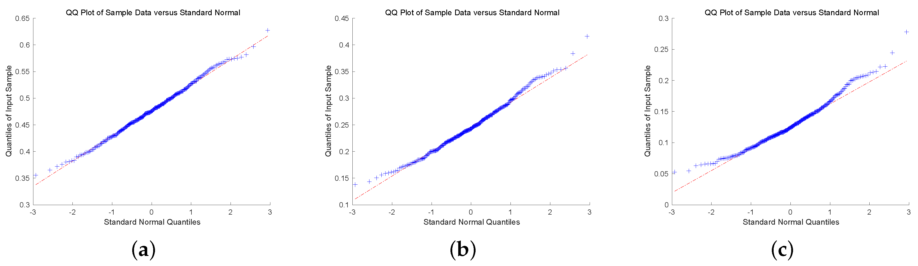
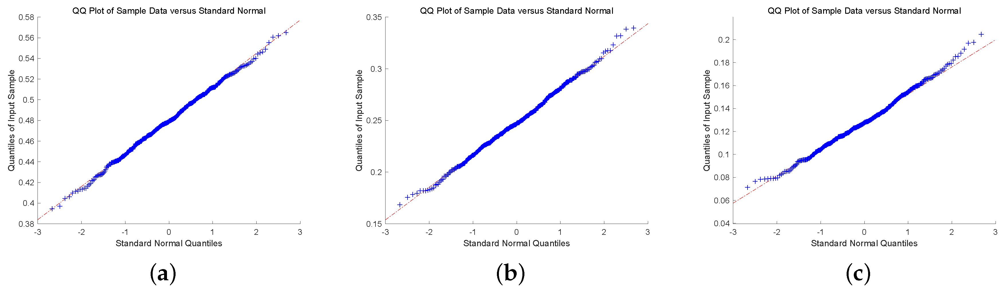
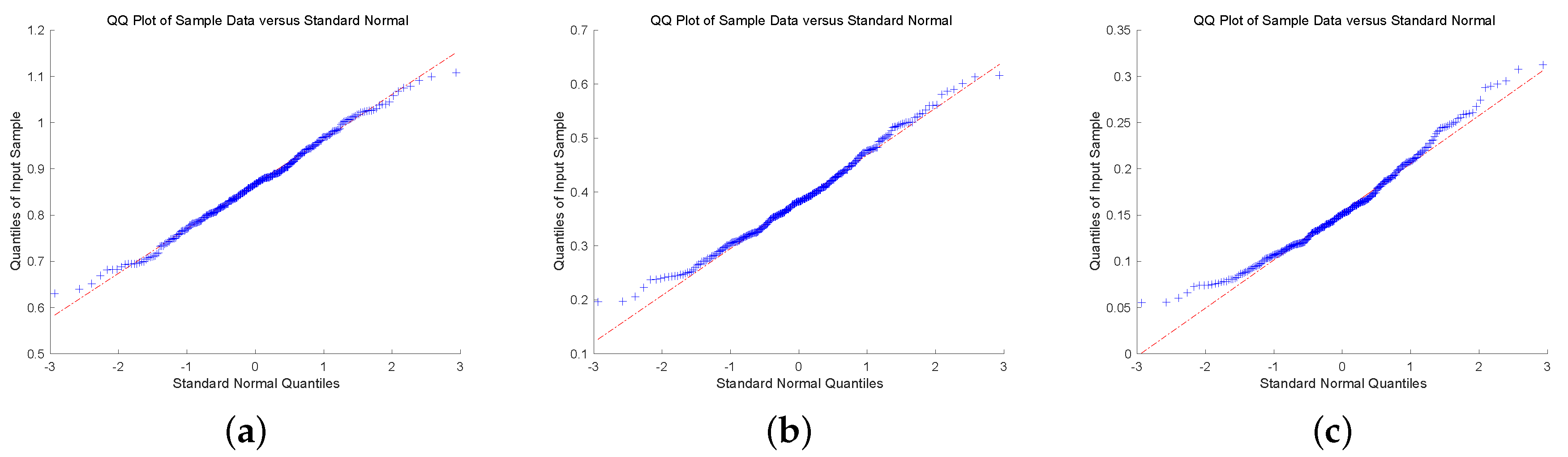
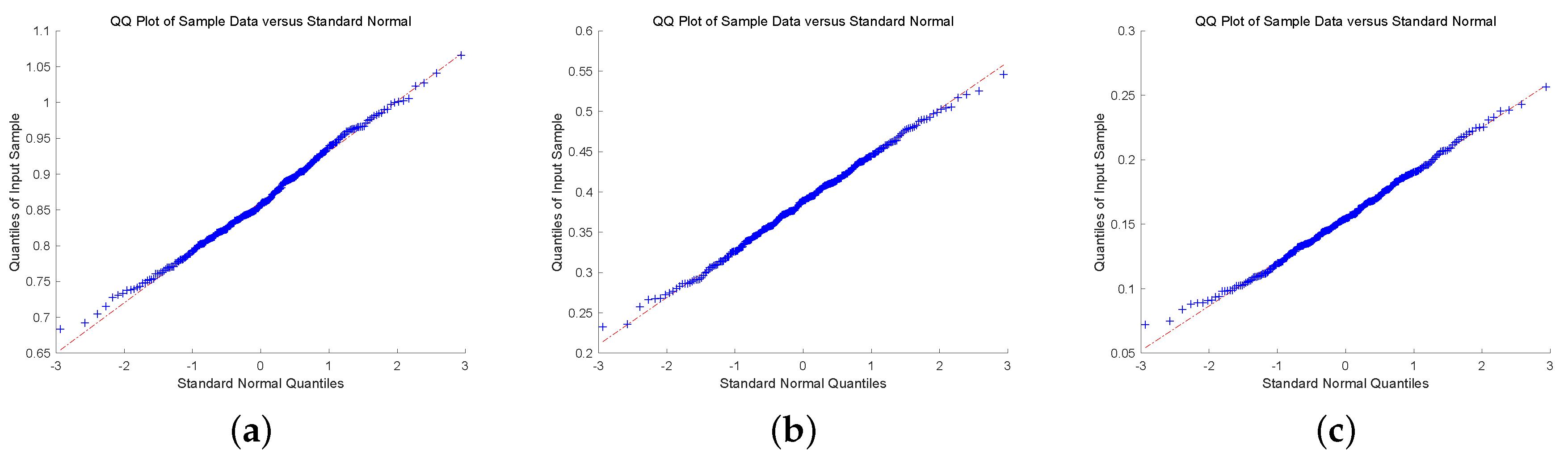
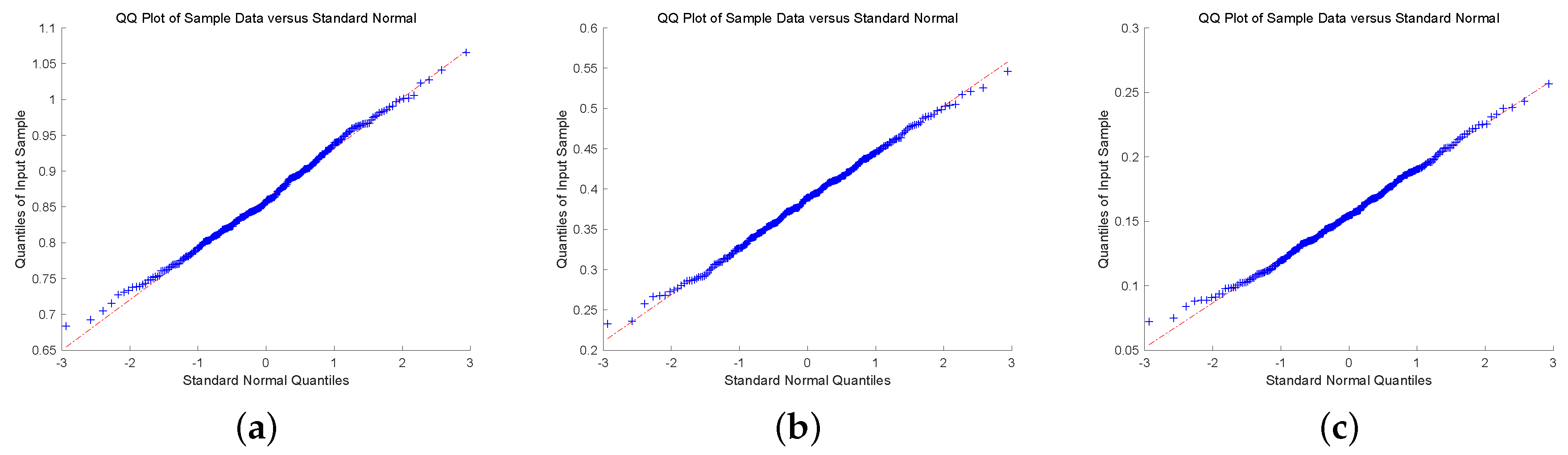
To check the asymptotic normality of the estimators, we present quantile-quantile plot (QQ-plot). QQ-plot displays each data point by marks, if the data points display a linear trend, then the distribution of the data is normal. To conclude this discussion, we show QQ-plot for different claim size densities and Gerber-Shiu functions with . In Figure 1 and Figure 2, we plot QQ-plot of Ruin probability for exponential claim size density with different u and T. The plot display an approximately straight line mean that the estimators are asymptotic normal. Then, we display the QQ-plot of ECS for Erlang(2) density in Figure 3 and Figure 4. The data point produces a straight line means that the estimators are asymptotically normal. In the end, we present QQ-plot of ED for combination-of-exponentials density in Figure 5 and Figure 6 with different u and T. The results manifest the Laguerre estimators are asymptotically normal. In addition, it can be observed from Figure 1, Figure 3 and Figure 5 with that the tails seem not converge to the normal distribution. Nevertheless, it is observed from Figure 2, Figure 4 and Figure 6 with that the results manifest asymptotic normality. In conclusion, we prove the asymptotic normality of our estimator as the value of T becomes large.
5. Conclusions
Recently, Zhang and Su [25] proposed a novel method for estimating the Gerber-Shiu function by Laguerre series expansion. Based on the observed information, we obtain the estimator of the Gerber-Shiu function. In this paper, we analyze the asymptotic normality of the Laguerre estimator mathematically and present some simulation experiments to support our result.
Author Contributions
Data curation, W.S.; formal analysis, W.S. and W.Y.; methodology, W.Y.; writing—original draft, W.S. All authors have read and agreed to the published version of the manuscript.
Funding
The research of Wenguang Yu was supported by the National Natural Science Foundation of China (No. 11301303), the National Social Science Foundation of China (No. 15BJY007), the Taishan Scholars Program of Shandong Province (No. tsqn20161041), the Humanities and Social Sciences Project of the Ministry Education of China (No. 19YJA910002), the Natural Science Foundation of Shandong Province (No. ZR2018MG002), the Fostering Project of Dominant Discipline and Talent Team of Shandong Province Higher Education Institutions (No. 1716009), Shandong Provincial Social Science Project Planning Research Project(No. 19CQXJ08), the Risk Management and Insurance Research Team of Shandong University of Finance and Economics, Excellent Talents Project of Shandong University of Finance and Economics, the Collaborative Innovation Center Project of the Transformation of New and old Kinetic Energy and Government Financial Allocation.
Conflicts of Interest
The authors declare no conflict of interest.
References
- Gerber, H.U.; Shiu, E.S.W. On the time value of ruin. N. Am. Actuar. J. 1998, 2, 48–78. [Google Scholar] [CrossRef]
- Asmussen, S.; Albrecher, H. Ruin Probabilities, 2nd ed.; World Scientific: Singapore, 2010. [Google Scholar]
- Gerber, H.U.; Landry, B. On the discounted penalty at ruin in a jump-diffusion and the perpetual put option. Insur. Math. Econ. 1998, 22, 263–276. [Google Scholar] [CrossRef]
- Tsai, C.C.L. On the discounted distribution functions of the surplus process perturbed by diffusion. Insur. Math. Econ. 2001, 28, 401–419. [Google Scholar] [CrossRef]
- Tsai, C.C.L. On the expectations of the present values of the time of ruin perturbed by diffusion. Insur. Math. Econ. 2003, 32, 413–429. [Google Scholar] [CrossRef]
- Yu, W.G. Some results on absolute ruin in the perturbed insurance risk model with investment and debit interests. Econ. Model. 2013, 31, 625–634. [Google Scholar] [CrossRef]
- Yu, W.G.; Huang, Y.J.; Cui, C.R. The absolute ruin insurance risk model with a threshold dividend strategy. Symmetry 2018, 10, 377. [Google Scholar] [CrossRef] [Green Version]
- Zhao, X.H.; Yin, C.C. The Gerber-Shiu expected discounted penalty function for Lévy insurance risk processes. Acta Math. Appl. Sin. 2010, 26, 575–586. [Google Scholar] [CrossRef]
- Xie, J.H.; Zou, W. On the expected discounted penalty function for the compound Poisson risk model with delayed claims. J. Comput. Appl. Math. 2011, 235, 2392–2404. [Google Scholar] [CrossRef]
- Zhu, H.M.; Huang, Y.; Yang, X.Q.; Zhou, J.M. On the expected discounted penalty function for the classical risk model with potentially delayed claims and random incomes. J. Appl. Math. 2014, 2014, 717269. [Google Scholar] [CrossRef] [Green Version]
- Yin, C.C.; Wang, C.W. The perturbed compound Poisson risk process with investment and debit Interest. Methodol. Comput. Appl. 2010, 12, 391–413. [Google Scholar] [CrossRef]
- Shen, Y.; Yin, C.C.; Yuen, K.C. Alternative approach to the optimality of the threshold strategy for spectrally negative Lévy processes. Acta Math. Appl. Sin. 2013, 29, 705–716. [Google Scholar] [CrossRef] [Green Version]
- Yin, C.C.; Yuen, K.C. Exact joint laws associated with spectrally negative Lévy processes and applications to insurance risk theory. Front. Math. China 2014, 9, 1453–1471. [Google Scholar] [CrossRef] [Green Version]
- Cai, C.; Chen, N.; You, H. Nonparametric estimation for a spectrally negative Lévy risk process based on low-frequency observation. J. Comput. Appl. Math. 2018, 328, 432–442. [Google Scholar] [CrossRef]
- Deng, Y.C.; Liu, J.; Huang, Y.; Li, M.; Zhou, J.M. On a discrete interaction risk model with delayed claims and stochastic incomes under random discount rates. Commun. Stat. Theory Methods 2018, 47, 5867–5883. [Google Scholar] [CrossRef]
- Dong, H.; Yin, C.C.; Dai, H.S. Spectrally negative Lévy risk model under Erlangized barrier strategy. J. Comput. Appl. Math. 2019, 351, 101–116. [Google Scholar] [CrossRef]
- Wang, W.Y.; Zhang, Z.M. Computing the Gerber-Shiu function by frame duality projection. Scand. Actuar. J. 2019, 2019, 291–307. [Google Scholar] [CrossRef]
- Yu, W.G.; Guo, P.; Wang, Q.; Guan, G.F.; Yang, Q.; Huang, Y.J.; Yu, X.L.; Jin, B.Y.; Cui, C.R. On a periodic capital injection and barrier dividend strategy in the compound Poisson risk model. Mathematics 2020, 8, 511. [Google Scholar] [CrossRef] [Green Version]
- Peng, X.H.; Su, W.; Zhang, Z.M. On a perturbed compound Poisson risk model under a periodic threshold-type dividend strategy. J. Ind. Manag. Optim. 2020, 16, 1967–1986. [Google Scholar] [CrossRef]
- Shimizu, Y. Nonparametric estimation of the Gerber-Shiu function for the Winer-Poisson risk model. Scand. Actuar. J. 2012, 1, 56–69. [Google Scholar] [CrossRef]
- Zhang, Z.M.; Yang, H.L. Nonparametric estimate of the ruin probability in a pure-jump Lévy risk model. Insur. Math. Econ. 2013, 53, 24–35. [Google Scholar] [CrossRef] [Green Version]
- Zhang, Z.M.; Yang, H.L. Nonparametric estimation for the ruin probability in a Lévy risk model under low-frequency observation. Insur. Math. Econ. 2014, 59, 168–177. [Google Scholar] [CrossRef] [Green Version]
- Zhang, Z.M. Estimating the Gerber-Shiu function by Fourier-Sinc series expansion. Scand. Actuar. J. 2017, 10, 898–919. [Google Scholar] [CrossRef]
- Zhang, Z.M. Nonparametric estimation of the finite time ruin probability in the classical risk model. Scand. Actuar. J. 2017, 5, 452–469. [Google Scholar] [CrossRef]
- Zhang, Z.M.; Su, W. A new efficient method for estimating the Gerber-Shiu function in the classical risk model. Scand. Actuar. J. 2018, 5, 426–449. [Google Scholar] [CrossRef]
- Shimizu, Y.; Zhang, Z.M. Asymptotically normal estimators of the ruin probability for Lévy insurance surplus from discrete samples. Risks 2019, 7, 37. [Google Scholar] [CrossRef] [Green Version]
- Yu, W.G.; Wang, F.; Huang, Y.J.; Liu, H.D. Social optimal mean field control problem for population growth model. Asian J. Control 2019, 1–8. [Google Scholar] [CrossRef]
- Peng, J.Y.; Wang, D.C. Uniform asymptotics for ruin probabilities in a dependent renewal risk model with stochastic return on investments. Stochastics 2018, 90, 432–471. [Google Scholar] [CrossRef]
- Yu, W.G.; Yong, Y.D.; Guan, G.F.; Huang, Y.J.; Su, W.; Cui, C.R. Valuing guaranteed minimum death benefits by cosine series expansion. Mathematics 2019, 7, 835. [Google Scholar] [CrossRef] [Green Version]
- Zhang, Z.M.; Yong, Y.D.; Yu, W.G. Valuing equity-linked death benefits in general exponential Lévy models. J. Comput. Appl. Math. 2020. [Google Scholar] [CrossRef]
- Abramowitz, M.; Stegun, I.A. Handbook of Mathematical Functions with Formulas, Graphs, and Mathematical Tables; National Bureau of Standards Applied Mathematics Series; US Government Printing Office: Washington, DC, USA, 1964.
- Cinlar, E. Probability and Stochastics; Springer: New York, NY, USA, 2015. [Google Scholar]
- Van Der Vaart, A.W. Asymptotic Statistics; Cambridge University Press: Cambridge, UK, 1998. [Google Scholar]
- Bongioanni, B.; Torrea, J.L. What is a Sobolev space for the Laguerre function system? Studia Math. 2009, 192, 147–172. [Google Scholar] [CrossRef] [Green Version]
- Dickson, D.C.M. Insurance Risk and Ruin; Cambridge University Press: Cambridge, UK, 2006. [Google Scholar]
Figure 1.
QQ-plot of RP for Exponential claim size density with : (a) ; (b) ; (c) .

Figure 2.
QQ-plot of RP for Exponential claim size density with : (a) ; (b) ; (c) .

Figure 3.
QQ-plot of ECS for Erlang(2) density with : (a) ; (b) ; (c) .

Figure 4.
QQ-plot of ECS for Erlang(2) density with : (a) ; (b) ; (c) .

Figure 5.
QQ-plot of ED for Combination-of-exponentials claim size density with : (a) ; (b) ; (c) .

Figure 6.
QQ-plot of ED for Combination-of-exponentials claim size density with : (a) ; (b) ; (c) .

© 2020 by the authors. Licensee MDPI, Basel, Switzerland. This article is an open access article distributed under the terms and conditions of the Creative Commons Attribution (CC BY) license (http://creativecommons.org/licenses/by/4.0/).
Share and Cite
MDPI and ACS Style
Su, W.; Yu, W. Asymptotically Normal Estimators of the Gerber-Shiu Function in Classical Insurance Risk Model. Mathematics 2020, 8, 1638. https://0-doi-org.brum.beds.ac.uk/10.3390/math8101638
AMA Style
Su W, Yu W. Asymptotically Normal Estimators of the Gerber-Shiu Function in Classical Insurance Risk Model. Mathematics. 2020; 8(10):1638. https://0-doi-org.brum.beds.ac.uk/10.3390/math8101638
Chicago/Turabian StyleSu, Wen, and Wenguang Yu. 2020. "Asymptotically Normal Estimators of the Gerber-Shiu Function in Classical Insurance Risk Model" Mathematics 8, no. 10: 1638. https://0-doi-org.brum.beds.ac.uk/10.3390/math8101638
Note that from the first issue of 2016, this journal uses article numbers instead of page numbers. See further details here.