Auto-Colorization of Historical Images Using Deep Convolutional Neural Networks

Abstract

Enhancement of Cultural Heritage such as historical images is very crucial to safeguard the diversity of cultures. Automated colorization of black and white images has been subject to extensive research through computer vision and machine learning techniques. Our research addresses the problem of generating a plausible colored photograph of ancient, historically black, and white images of Nepal using deep learning techniques without direct human intervention. Motivated by the recent success of deep learning techniques in image processing, a feed-forward, deep Convolutional Neural Network (CNN) in combination with Inception- ResnetV2 is being trained by sets of sample images using back-propagation to recognize the pattern in RGB and grayscale values. The trained neural network is then used to predict two a* and b* chroma channels given grayscale, L channel of test images. CNN vividly colorizes images with the help of the fusion layer accounting for local features as well as global features. Two objective functions, namely, Mean Squared Error (MSE) and Peak Signal-to-Noise Ratio (PSNR), are employed for objective quality assessment between the estimated color image and its ground truth. The model is trained on the dataset created by ourselves with 1.2 K historical images comprised of old and ancient photographs of Nepal, each having 256 × 256 resolution. The loss i.e., MSE, PSNR, and accuracy of the model are found to be 6.08%, 34.65 dB, and 75.23%, respectively. Other than presenting the training results, the public acceptance or subjective validation of the generated images is assessed by means of a user study where the model shows 41.71% of naturalness while evaluating colorization results.

1. Introduction

One of the recommended techniques to safeguard a culture is through the documentation, the dissemination, and enhancement of cultural heritage (CH) [1]. Tangible or intangible cultural heritage such as historical images reveal an undeniable expression, richness, and diversity of cultures [2,3]. Besides the ancient techniques which were used to protect the historical images, a new technological paradigm such as 3D modeling or auto-colorization provides a fascinating visual appearance [4,5].

In past when the photography was first invented, only black and white images were available due to technological limitations. However, nowadays color photography becomes the part of lifestyle. There are a lot of memories and connections between present and past with historical photography. It would be more interesting to convert them to colored ones for enhancing hidden meanings and visual appealing. The way people used for colorization was manual painting or using Photoshop and was time consuming. Nepalese Painting can be found in the form of wall paintings, cloth paintings, or manuscripts as traditional techniques from centuries. However, now, using artificial intelligence (AI) and deep learning, the process can be carried out automatically. Given a historical, heritage, or cultural gray-scale input image, as shown in Figure 1, the goal of this research is to produce an auto-colorized image using an algorithm based on deep convolutional neural network (CNN).

Colorization, which is the process of adding colors to grayscale images or monochrome videos, has been an active research field. Conventionally, optimization methods that optimize every pixel based on user inputs or reference images are used as the mainstream for colorization. However, with the rapid advance of deep learning in recent years [6,7], methods that use a CNN to automatically perform colorization have dominated the current trend. In such methods, deep networks are trained with a large number of images so they can output a colorized image given a grayscale image. This research builds a colorization deep neural network that can colorize cultural, heritage, and historical images of ancient Nepal that are black and white in just a few seconds without user-intervention. We propose a network model which integrates deep CNN with Inception ResNetV2, a most powerful network having highest accuracy among all other inception models. Inception ResNetV2 is used as a global feature extractor for better semantic understanding in the colorization process. CNN combines both local and global image features. Local features are based on small areas of pixels while a global feature resembles the whole content in the image so that the model can understand what is in the picture. For color conversion, International Commission on Illumination (CIE) L*a*b* color space is employed where model predicts chroma (a*, b*) values given Luminance value. More specifically, Red, Green, and Blue (RGB) image is first converted to CIE L*a*b* color space. This is because the luminance (L) channel acts as grayscale input to our model. The two channel outputs a* and b* represent colors for the grayscale images. A basic concatenation between input and output is required to obtain three-channel image. Finally, L*a*b* to RGB conversion is made to get an image in RGB color space.

Mean Squared Error (MSE) and Peak Signal-to-Noise Ratio (PSNR) are used as loss objective functions to update the model parameters. On the other hand, a subjective measure based on Mean Opinion Score (MOS) is used for model validation where percentage value is used to evaluate the naturalness of colorization. Our main contributions are as follows:

• We analyze the colorization process on the dataset using the CNN-integrated model with Inception ResNetV2.
• Several pieces of research have been reported in the literature on colorization for black and white images with varieties of datasets, including heritage images of Japan, Vietnam, France (Pablo Picasso’s), ImageNet dataset, SUN dataset (4.0.0, Princeton, USA), CIFAR-10 (3.0.2, Toronto, Canada), etc. Inspired by these, we try to apply recent trends of deep learning approaches on our own dataset.
• We perform an objective and subjective evaluation of the model using various metrics such as MSE and PSNR.
• The proposed framework can be considered a base-model for the colorization of ancient images.

The rest of the paper is organized as follows: the literature review is presented in Section 2. The used methodology and its underlying techniques are provided in Section 3. The results of the work are discussed in Section 4 while the concluding remarks followed by limitations and future directions are presented in Section 5.

2. Related Works

Colorization of images itself is an ambiguous task since it doesn’t have unique solution. Though various research that have been carried in the field of image colorization, approaches to such tasks can be categorized into three groups: scribble-based, example-based, and learning-based.

Scribble-based colorization approaches interpolate colors in the grayscale image based on color scribble produced by an artist where scribbles are propagated through the remaining pixels of the image. In [8], the authors applied this method to some stationary images and video sequences. However, it was found that the scribble based method had some problems such as a color blending effect at edges of an image and dependency of performance was based upon human skills which were improved in [9,10]. An example-based learning approach, where color transform between images was carried out by referencing one image’s color information to another by using the color correlation method [11], where pixel intensity values are calculated from different neighborhood values to match the pixels of the reference and grayscale target image [12,13]. Example-based colorization gives best results only when we were able to find proper color image, which is given as one of the inputs to the algorithm. Learning-based methods in [14,15,16,17] applied various machine learning models and algorithms to learn complex patterns and features present in the image by using a large dataset fed to the model [14,15,16,17]. Learning-based techniques are automatic and remove the drawbacks of manual color assignments.

In recent years, CNN based approaches are widely used for image colorization purposes. In [16,18], authors presented two-stream architecture to elaborate the simultaneous extraction of local and global features. Such extracted features were then fused together. These kinds of methods use CNN to extract features from a given grayscale image and colorize it based on the extracted features. However, qualitative evaluation of those algorithms requires human participants to determine the difference between real and colorized images. Colorization of grayscale images was defined as a classification problem using pre-trained models VGG with some modifications for grayscale images where hypercolumns were used to predict two distributions: hue and chroma for each pixel. Looking at the recent trends in deep learning, CNNs become a vital player to handle diversified tasks such as image colorization, classification, image-labeling, restoration and style transfer with top-5 errors below 5% on the ImageNet challenge [19,20].

The concept based on CNN for colorizing grayscale historical images was applied by Lizuka et al. [18], where colorization was performed along with classification. They fused both local and global features at the fusion layer where the global feature network is similar to classification tasks in order to understand semantic context present in the image. In [19], the authors also applied the classification based CNN model to analyze loss functions: regression loss (L2 loss) and cross-entropy (CE). Furthermore, they also analyze the better results using the conditional Generative Adversarial Network. However, they applied the CIFAR-10 dataset. In [21], the authors applied Vietnamese heritage repository for classification purposes using CNN and AlexNet (2012, New York, USA). An automatic cartoon colorization based CNN model was proposed by Varga et al. [22] using CNN where colorization is considered as multinomial classification instead of regression. Baldassarre et al. [23] also applied the concept of fusion layer where CNN extracts low and mid-level features and Inception ResNetV2 extracts global features with MSE as an objective function. However, they used 60K images as part of the ImageNet dataset. This method also applied qualitative evaluation using human participants asking them to differentiate colorized and real images. This study specially focuses on colorization of black and white historical, cultural, and heritage photographs of ancient Nepal.

3. Methodology

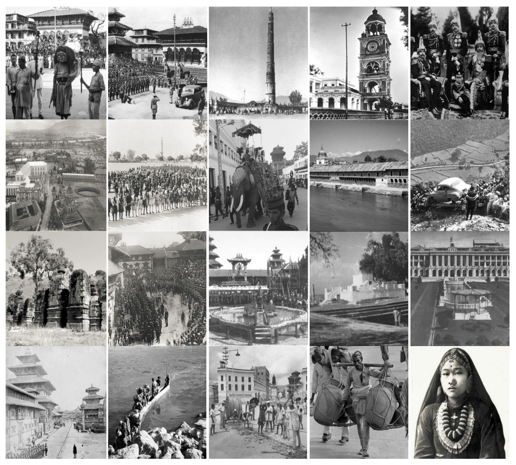
3.1. Dataset Construction

In order to train, test, and validate the colorization model, we create a dataset consisting of the heritage, historical, and cultural image repositories of Nepal. Most of the images were collected from the internet and are publicly available. Some such sources are Vintage Nepal, the Nepal picture library, the Department of Archaeology of the government of Nepal, cultural heritage blog spots, Getty images, etc. There are a wide variety of datasets for the colorization of grayscale images including the ImageNet dataset. To the best of our knowledge, no historical, cultural, and heritage image datasets in the context of ancient Nepal have been developed and used for colorization purposes. In Nepal, colorization of old historical, cultural heritage such as Thangka and Paubha (religious paintings that are made by the Newar people of Nepal) are still being colorized with manual painting or using Photoshop. Colorization of images can be seen in the form of painting the religious paintings of Hindu and Buddhist culture. Those traditional paintings can be found in the form of wall paintings, cloth paintings, or manuscripts. They used conservative technique, style, and iconography in their works for centuries. However, performance depends upon the skill of the artist. These images have enormous historical value and have recorded people’s lifestyles for more than a century. Most such images are black and white rather than color, and photographic technologies used a century ago are quite different from today. Thus, an automatic colorization technique is proposed that uses machine learning to create vibrant and realistic colors for those images. About 1.2 K images of size 256 × 256 including some validation images were collected with a variety of sources such as people and lifestyle, culture and religion, festivals, arts and architecture, museums and galleries, industries and economy, geography, history, paintings, statues, temples, monasteries, old squares, monuments, etc.

Table 1. Cultural, Heritage, and Historical Image Dataset.

Dataset	Culture	Heritage	History	Total
Test (Grayscale)	44	65	41	150
Train (RGB)	305	350	315	970

gives the summary of collected datasets. In addition, some sample images taken from the test dataset used for colorization are shown in Figure 2.

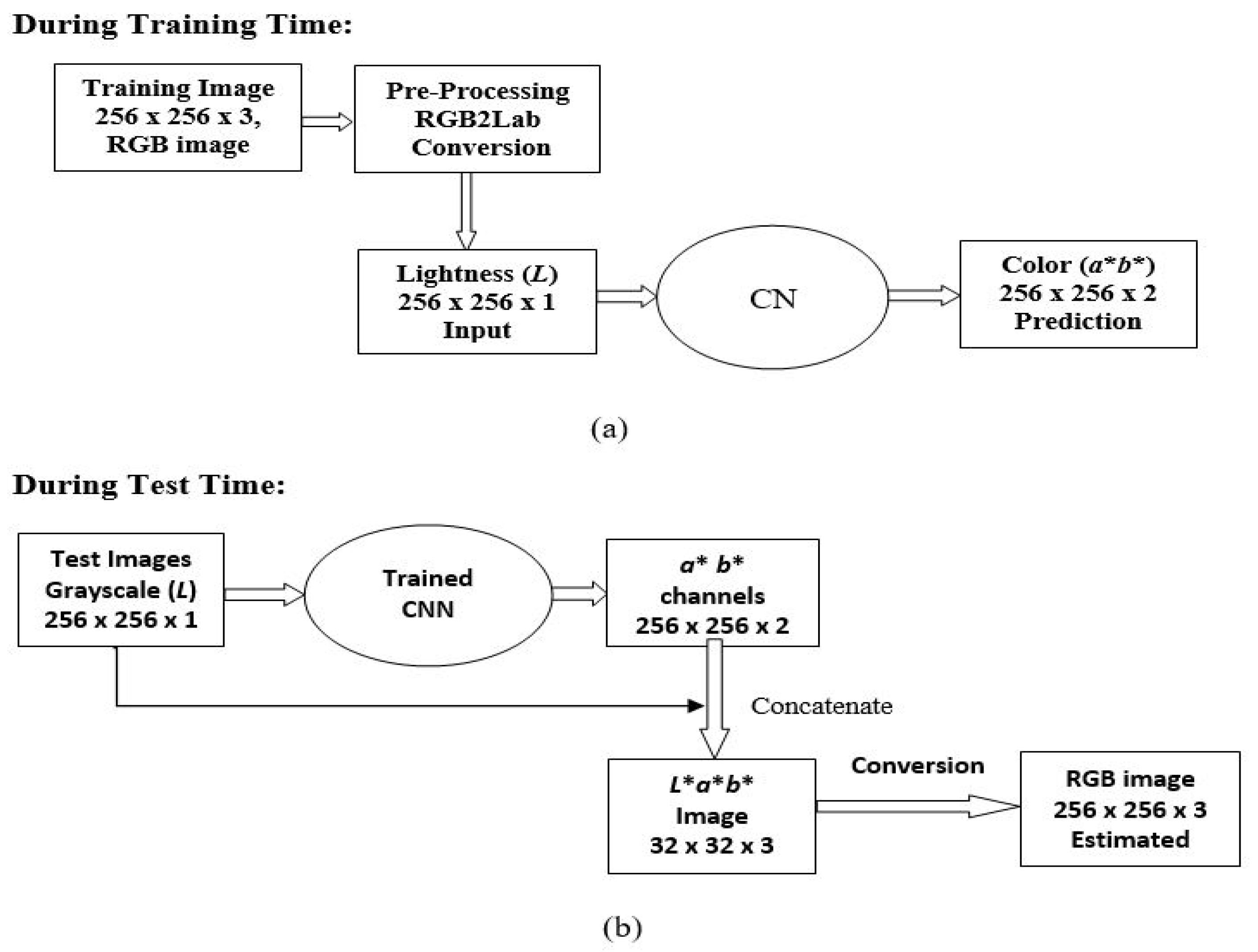
3.2. Pre-Processing Images

First of all, a random collection of both RGB and black and white images was made for train and test datasets, respectively. Images having unusual aspect ratios—low-resolution and high degradation—were removed in the first stage. Then, cropping and resizing are applied to fix the resolution to 256 × 256. Then, 256 × 256 × 3 images were converted to CIE L*a*b* color model because this model converts RGB images into the three corresponding color layers; two chroma components (a* and b*) and a luminance (L that contains image features) component. An image in L*a*b* color space has one layer for luminance, and packed three RGB layers into two chroma layers. This illustrates that the original luminance value present in the image can be used for final color prediction. Here, the model just needs to predict two chroma channels from a given grayscale value. After that, pixel values for L (Lightness/Luminance), a* (Green-red), and b* (Blue-yellow) components are scaled and centered such that obtained values are between −1 and 1.

The CNN model is implemented as a learning pipeline, which takes pre-processed grayscale images as input. During training time, the luminance (L channel) is fed to the model as input. The a* and b* channels are extracted as the target values. During testing time, the model accepts a 256 × 256 × 1 black and white image. It generates two arrays, each of dimension 256 × 256 × 1, corresponding to the a* and b* channels of the CIE L*a*b* color space. With the luminance component as an input, the chrominance (a*b*) is estimated through the model to restore fully colorized images, which is a mapping from luminance to chrominance. The three channels are then concatenated together to form the CIE L*a*b* representation of the predicted image. Finally, L*a*b* to RGB conversion is applied as the final output as shown in Figure 3.

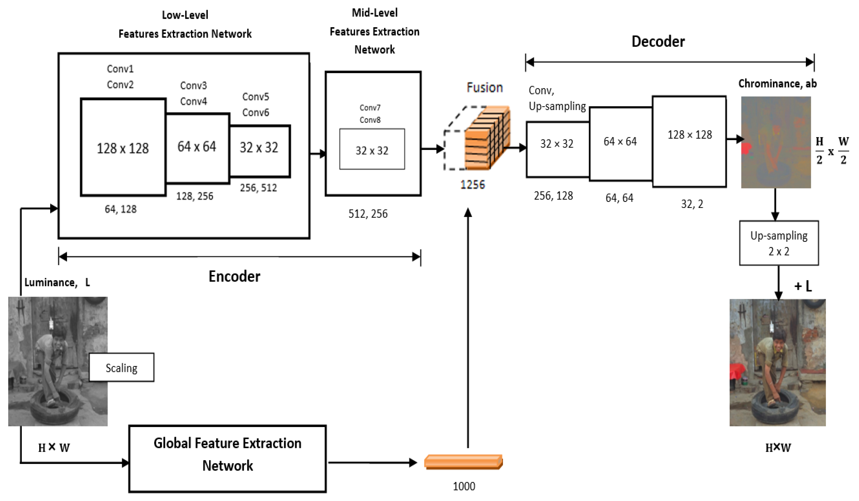
3.3. CNN Model Architecture

The proposed CNN model has four main parts: Encoder, Global features extractor, Fusion, and Decoder. The basic flow in the architecture is as follows: Initially, a set of low-level features are extracted from an image. Low-level features are then used to compute mid-level image features. Global image features are extracted from a global feature extractor network (Inception ResNetV2). The “fusion layer” fuses both “mid-level” and the “global features”. The decoder takes the output from the fusion layer, which acts as the “colorization network” that outputs the final chrominance map as depicted in Figure 4.

The network uses encoder–decoder architecture, and it consists of a series of convolution layers which are a set of small learnable filters that look for specific local patterns in input images and generate activation maps. As we reach deeper levels, higher-level features are extracted. CNN consists of layers realizing a function (f) of the form:

$$f=\tilde{\sigma }(b+W_g)$$

(1)

where $g\in R^q$ is an input and $f\in R^p$ is an output of every layer. W is a weight matrix of size $p\times q$, $b\in R^p$ is a bias vector, and $\tilde{\sigma }:R^p\to R^p$ is a transfer function which is nonlinear. The values of learnable parameters W and b are continuously updated through back-propagation. Here, loss indicates the difference between network prediction and the real image (from training data).

Table 2. Details of network architecture; Left: encoder network, mid: fusion network, right: decoder network.

Encoder				Fusion				Decoder
Layer	Kernel	Stride	Outputs	Layer	Kernel	Stride	Outputs	Layer	Kernel	Stride	Outputs
conv	3 × 3	2 × 2	64	fusion	-	-	256	conv	3 × 3	1 × 1	128
conv	3 × 3	1 × 1	128	conv	1 × 1	1 × 1	256	upsamp	-	-	128
conv	3 × 3	2 × 2	128					conv	3 × 3	1 × 1	64
conv	3 × 3	1 × 1	256					conv	3 × 3	1 × 1	64
conv	3 × 3	2 × 2	256					upsamp	-	-	64
conv	3 × 3	1 × 1	512					conv	3 × 3	1 × 1	32
conv	3 × 3	1 × 1	512					conv	3 × 3	1 × 1	2
conv	3 × 3	1 × 1	256

further details the network layers.

3.3.1. Encoder Unit

Both low and mid-level feature networks act as encoder units. Encoder uses 6-layered CNN to extract “low-level” features from the input image using 3 × 3 kernels. The input to encoder unit is H × W gray-scale images and results an H/8 × W/8 × 512 dimension feature map. To reduce the size of feature maps, we have used increased stride at each convolutional layers rather than max-pooling. To preserve the original image size, padding is used at each layer; this is because the output is reduced by 50% of the input size at each layer (if stride = 2). Convolutional kernels of size 3 × 3 are used exclusively throughout the network, and a padding of size 1 × 1 is used to make output and input sizes same. Every odd layer (1st, 3rd, and 5th) applies a stride of 2, so as to reduce dimension of their output by half. The ultimate result is a reduction in the number of computations required. An overview of the architecture of low and mid level feature extraction network is shown in Table 2.

The low-level features are further processed with two convolutional layers to obtain mid level features. Here, 256-channel mid-level features are extracted from 512-channel low-level features to produce the output volume of size H/8 × W/8 × 256, (i.e., 32 × 32 × 256) where H and W are the original image height and width respectively. Low level feature extraction is mainly concerned with extracting local texture, objects, and descriptions at a given location from images. There may be multiple, largely independent descriptions, such as edge fragments, spots, curves, line fragments, etc. As we move to a mid-level feature extraction network, the model can detect more complex patterns. The mid level feature extraction is mainly concerned with extracting descriptions of the scene extracted at a low level in a more symbolic form or describing a certain position and shape of the scene.

3.3.2. Global Feature Extractor

High-level features are used to understand the semantic context at an image level so that the network can get a sense of what is in the picture. At this level, the network is able to match each object with the appropriate color. To extract an image embedding, the inception model is used. We have applied the Inception-Resnet-V2 model, neglecting the last Softmax layer for global feature extraction. This model itself is a CNN that can classify 1000 object categories and is the most powerful network among all inception models [24]. Initially, the input image is scaled to 299 × 299. Then, the image (i.e., luminance component) is stacked on itself three times to obtain a three (RGB) channel image and hence matches the exact dimension for the Inception network. Next, the resulting image is fed to the network and the output of the last layer (1000 × 1 × 1) before the Softmax function is extracted.

3.3.3. Fusion Layer

At the fusion layer, the output of convolutional layers of the encoder is fused with the output of the Inception embedding. This allows for merging local information with global information present in the image. The fusion layer combines the global image features, a 1000-D vector, with the output of mid-level image features having size H/8 × W/8 × 256. A feature vector of 1000 dimension from Inception is initially fed to a fusion layer which replicates it H/8 × W/8 times and attaches it to the feature volume output by the encoder unit along the depth axis [18,23]. This allows us to obtain a single volume with the encoded image and the mid-level features of shape H/8 × W/8 × 1256 (i.e., 32 × 32 × 1256). Mirroring and concatenating the feature vector several times ensures that the semantic context present in the feature vector is uniformly distributed among all spatial regions of the image. Lastly, 256 convolutional kernels of size 1 × 1 are applied to generate a feature vector of size H/8 × W/8 × 256. The output of the fusion layer for mid-level coordinates ($x,y$) as:

$$y_{x,y}^{fusion}=\sigma \left(b+W\left[\begin{array}{c}{y}^{global}\\ y_{x,y}^{mid}\end{array}\right]\right)$$

(2)

where $y_{x,y}^{fusion}\in R^{1256}$ is the fused feature at ($x,y$), $y_{x,y}^{global}\in R^{1000}$ is the global feature vector, $y_{x,y}^{mid}\in R^{256}$ is the mid-level feature at ($x,y$), W is a weight matrix, and $b\in R^{1256}$ is a bias. Both W and b are learnable part of the network.

3.3.4. Decoder Unit

The decoder uses fused features in order to estimate the output i.e., chrominance components of the image. Fused features are then processed by a series of convolutions and up-sampling layers. The output of the fusion layer, a 32 × 32 × 256 volume, is fed to the decoder initially and then multiple convolutional and up-sampling layers are applied to obtain a final chrominance map with volume H × W × 2. Up-sampling is performed using the basic 2D-nearest neighborhood method to increase output volume by twice its initial volume. The architecture is shown in Figure 4. This chrominance map is concatenated with the luminance (L) component of the input image to produce an image in CIE L*a*b* color space, which is then converted to RGB color space to get full three channel color images as output.

3.4. Optimization and Learning

The main objective of optimization is to find optimal values to model parameters by minimizing cost (or loss) function. To measure the model loss quantitatively, there are two different attempts made, one is Mean Square Error (MSE) and another is Peak Signal-to-Noise Ratio (PSNR). MSE is calculated between the estimated pixel colors in a*b* space and their ground truth value. For an image P, the MSE [23] is given by Equation (3):

$$C(P,\beta )=\frac{1}{2HW}\sum _{k\in \{a,b\}}\sum _{i=1}^H\sum _{j=1}^W{(P_{k_{i,j}}-{\tilde{P}}_{k_{i,j}})}^2$$

(3)

where $C(P,\beta )$ is the loss function, $\beta$ represents model parameters, $P_{k_{i,j}}$ and ${\tilde{P}}_{k_{i,j}}$ denote the i, j: th pixel value of the k: th components of predicted and ground-truth image, respectively.

For each iteration, the loss is backpropagated to update the model parameters $\beta$ using the Adam Optimizer [25] with a global learning rate $\eta =0.001$. We have applied the rectified linear unit (ReLU) as an activation function at each of convolutional layers, except at the last layer that uses a hyperbolic tangent (tanh) function. ReLU introduces nonlinearity to the system. It helps to alleviate the vanishing gradient problem and doesn’t saturate.

Peak Signal-to-Noise Ratio (PSNR) is another objective quality assessment metric proposed in this paper to measure the quality of predicted color images. It is the approximate estimation to human perception of reconstruction quality. Because the human eye is most sensitive to luma information, we compute PSNR only on the luma channel, where luma represents a weighted average (L = 0.3 R + 0.59 G + 0.11B) of R, G, and B channels. The PSNR calculates the peak signal-to-noise ratio, between colorized image and corresponding ground truth image. We always desire higher value to the PSNR for better quality of the reconstructed image. PSNR (in dB) is expressed as [26]:

$$\begin{array}{cc}\hfill PSNR& =10lo{g}_{10}\left(\frac{peakva{l}^2}{MSE}\right)\hfill \\ \hfill & =20lo{g}_{10}\left(peakval\right)-10lo{g}_{10}\left(MSE\right)\hfill \end{array}$$

(4)

where peakval (Peak Value) is the maximum value to the pixel intensity of an image. Peak value to a pixel is 255 for 8-bits pixel representation. Generally, PSNR fits in the range of 30 to 50 dB [26] for image or video quality reconstruction or degradation, assuming a bit depth of 8 bits. PSNR uses MSE in the denominator. The lower the error, the higher the PSNR will be.

4. Results and Discussion

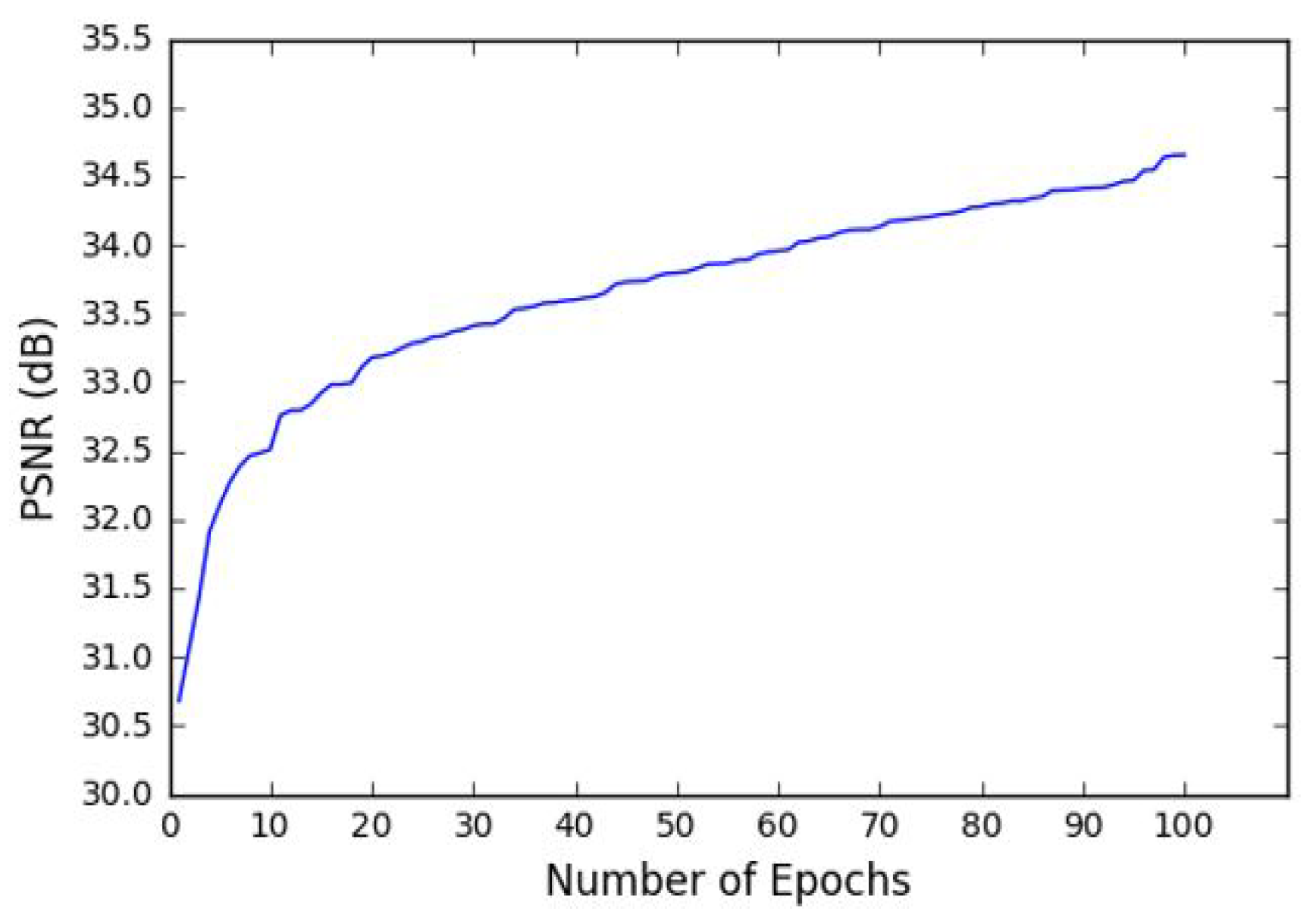
4.1. Training

Approximately 1.2 K images were used in the dataset, out of which 85% were used for training purposes while the remaining 15% were used for model testing. Basically, the split ratio depends on two aspects: the total number of samples in the dataset and the actual model we are training. As such, we have performed dozens of experiments with varying split ratios (80:20, 90:10, and 85:15), different batch sizes, and epochs. In addition, we tested colorization results with two optimizers Adam and Rmsprop. Increasing epochs beyond 200 results in memory overflow and exceeds the time limitation of 12 h provided by the Google Colab environment (NVIDIA Tesla K80, 12 GB RAM) (Kepler 2.0, Santa Clara, CA, USA). The best result was with an 85:15 split ratio, batch size of 20, 200 epochs, and with Adam optimizer. The results presented in this paper are taken from the test and the validation set. To reduce possible overfitting, some data augmentation techniques such as rotate, flip, shear, etc. were used. This way, each image will never be the same, thus improving the learning rate. The Adam optimizer was used during training. To speed up the computations, the network was trained and tested using the Google Colab environment, which is Google’s free cloud service for AI developers. With Colab, we can develop deep learning applications on the NVIDIA Tesla K80 Accelerator GPU for free. The higher value of batch size such as 50–100 resulted in GPU memory outage. The batch size of 20 gave proper results from the proposed model. The total number of learn-able parameters was about 6.5 M. Coding was carried out with Python 3.6. The Jupyter Notebook (Version 6.1.5), an open-source web application is used as an Integrated Development Environment (IDE). Some library packages such as Tensorflow, Keras, OpenCV, Matplotlib, Numpy, Skimage, Scipy, etc. were used extensively [16,27,28].

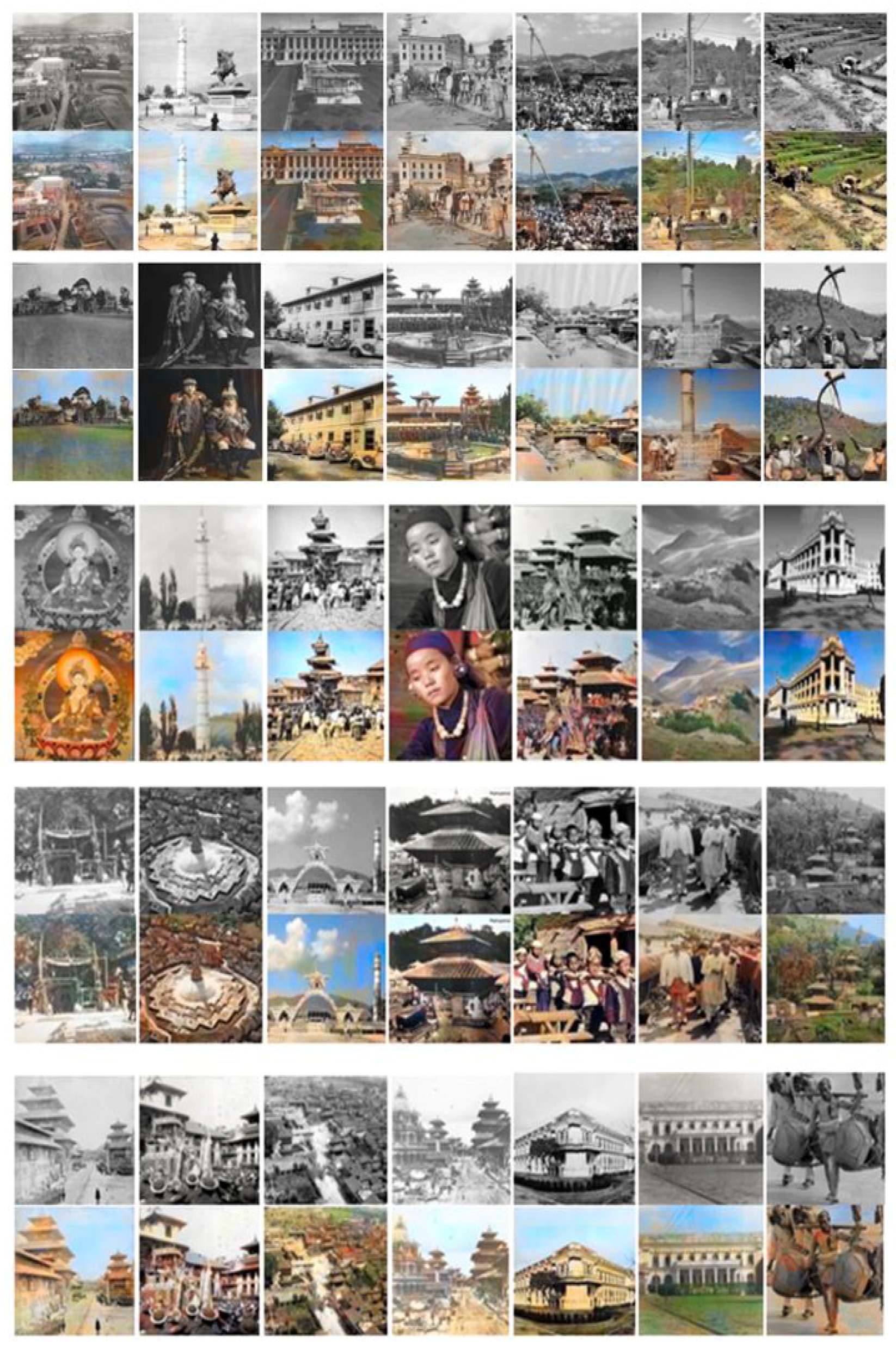
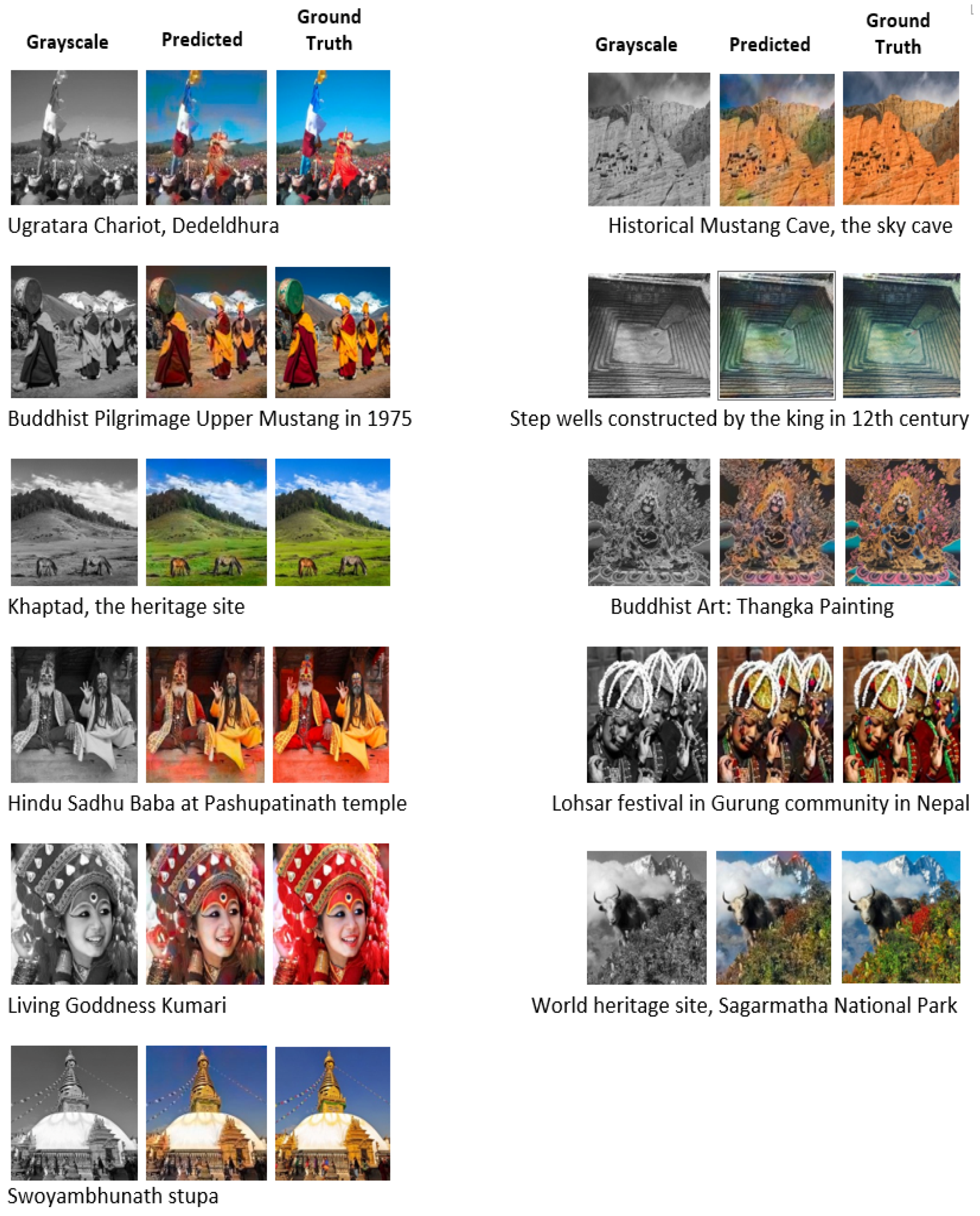
4.1.1. Colorization Results on Test Images

Once trained, images from the test dataset were fed to the model. The results seemed good for some images, generating near realistic pictures. However, poor performance for some images might be due to the small data size and variability of images in the training set. For example, the color of the dressing of the Rana dynasty was not recognized by the model. Thus, poor coloring results were obtained. The network performs better when certain image features appear. For instance, natural elements such as the sky, trees, and rivers seem to be well recognized. However, specific objects are not always well colored. A test dataset of 150 images was applied. Figure 5 illustrates results for some test examples where the network produced their colorized version.

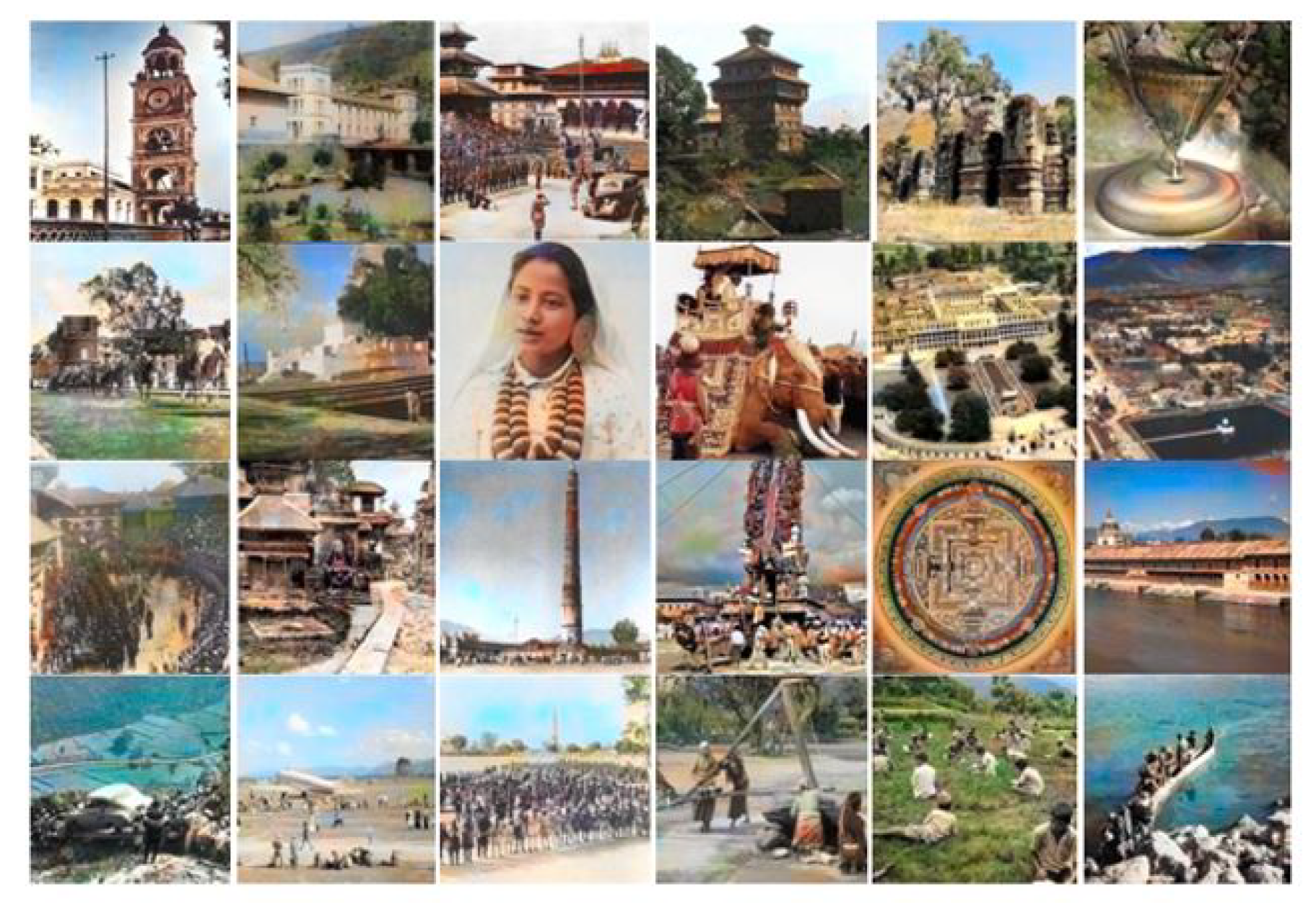
4.1.2. Colorization Results on Validation Images

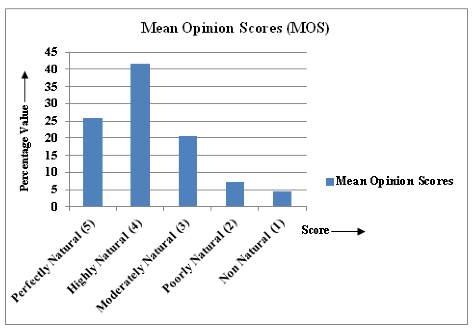
The validation set was used for tuning and unbiased evaluation of the performance of the model such that we can assess how well the network is currently performing. About 20 were used for validation purposes, and each such image has its ground truth version. Near realistic colorization, results were obtained on the validation dataset without overfitting e.g., an image of the Khaptad National Park. Each of the objects in the image such as sky, green-land, and the horse were clearly understood by the model. Figure 6 shows the comparison of the results obtained from our colorization network with original images.

The Mean Squared Error (MSE) was taken as a loss function during model training. Adam with an initial learning rate LR = 0.001 was used as an optimizer. Choosing a proper batch size was difficult. A large amount of training was conducted to find the proper value of batch size. Initially, training was performed with parameters having varying batch sizes and epochs. Later, it was found that a batch size of 20 gives proper results. Figure 7 shows the plot of loss and accuracy versus the number of epochs of the trained model. It was found that a loss of 19.11% and 67.10% of model accuracy (see

Table 3. Results of loss and model accuracy for a varying number of epochs with integrating the Inception model.

Model	MSE	Model Accuracy	Batch Size	Epoch	Training Time (hours)
CNN with Inception	6.08%	75.23%	20	200	6.25
CNN with Inception	19.11%	67.10%	20	100	2.61

). Before taking the batch size of 20, we have applied a decreasing batch size of 10 as well as increasing batch size 25, but the network could not converge on loss and accuracy.

Therefore, a batch size of 20 was applied. In addition, the number of epochs was further increased to 200. The plot of loss and accuracy with a batch size of 20 with 200 epochs is shown in Figure 8, where MSE loss of 6.08% and 75.23% model accuracy were obtained. It was found that, with an increased number of epochs, there was a gradual decrease and increase in loss and accuracy, respectively, giving more realistic and better colorization results. However, training with a higher number of epochs and with a higher size of the dataset in the cloud GPU environment also has high computational complexities such as insufficient memory space and higher training time. During experiments, it was also found that the model without inception integration gave worse results than the model with inception integration.

Furthermore, Peak Signal-to-Noise Ratio (PSNR) was used as another objective image quality metric for model validation. As shown in Figure 9, the PSNR of colorized results were calculated and found to be 34.65 dB. It can be seen that the PSNR of results in this research is comparable to other state-of-the-art methods such as presented by the authors in [16,17,27]. Cheng et al. [16] found PSNR up to 33 dB, Larsson et al. [17] found 35 dB, and Liu et al. [27] found PSNR in the range of 39 dB to 41.4 dB, which indicates that the employed model was good in terms of image color quality.

4.2. User Study

A quantitative measure of the performance of the model was obtained using MSE and PSNR, which is not sufficient to measure image color quality. A subjective quality assessment technique should be used which shows how the appearance of recolored images looks to the human eye. This evaluation was carried out by means of a user study [17,18,23] called Mean Opinion Score (MOS) [29]. Twenty-nine colorized images were shown to users one by one, and each user was asked how to make sense of “Natural or Un-natural”, “Original or Re-colored”. Indications were given to the users to use their gut feeling and not try to spend too much time looking at the details of the images. Twenty-one different users have participated in the poll. We have chosen some best-recolored results for human visual perception. The MOS has been used for subjective quality assessment i.e., to test the naturalness of colorized images (see Figure 10). Both male and female, professional, and non-professional viewers rated the visual quality of colorized images obtained from the model. The MOS is generated by averaging the result of a set of standard, subjective tests. MOS is an indicator of the perceived image color quality. MOS of 1 is the worst image quality which is indicated by non-natural and 5 is the best, which is indicated by being perfectly natural.

It was observed that an average of 25.94% of users rank colorized images as perfectly natural, 41.71% as highly natural, 20.51% as moderately natural, 7.38% as poorly natural, and 4.43% as non-natural. The plot of scores and their percentage value are shown in Figure 11 Some previous works on colorization such as described in [16,23] obtained 32% and 45.87%, respectively. They both used only two scores: natural and un-natural for subjective evaluation of colorized results. The authors in [16] used 10K and the authors in [23] used 60K images as part of the ImageNet dataset. In this regard, MOS used in this research gave valid results subjectively.

4.3. Comparative Study

As evident from the PSNR results, our framework offers image colorization with improved or comparable performances as compared to various existing approaches from enhanced signal energy perspectives. In [16], the authors train a CNN to map from a grayscale input to a distribution over quantized outputs. The approach basically translated the colorization uncertainty into a classification-only task, where the diversity of the colors was increased by class-rebalancing during the training phase, whereas the proposed framework deals with global features with the help of Inception ResNetV2 with a similar level of PSNR. The superiority of the color enhancement of our method is also apparent as it offers similar image color qualities with reduced PSNR as compared to the local semantic information-assisted global classifier approach [27]. Apart from the energy enhancement viewpoint, the proposed framework offers even higher user satisfaction than existing methods [16,23]. The CNN model introduced in this work performed precise coloring on various important image components including the sea, land, and trees. The results suggest that MOS-based subjective quality assessment carried in our work captures the users’ perceptions more precisely than the other methods. Since the images are specific to Nepal’s culture, heritage, lifestyle, and history, they have some specific patterns, and some images have a low resolution with unusual length to width ratio. Understanding the semantic information was challenging due to blurred edges and missing color values in the image pixels. Nevertheless, our method provides plausible coloring results.

5. Conclusions and Future Work

5.1. Concluding Remarks

Colorizing images is a deeply fascinating problem. In this research, the auto-colorization of black-and-white historical, cultural, and heritage images using CNN was studied. A CNN auto-colorization model was developed where local image features were fused with semantic (global) image features. The model was trained on a dataset of 1.2 K images of ancient Nepal created by us. It was found that the model with Inception ResNet v2 integration with basic CNN performed better than without integration. We used MSE and PSNR as objective measures and obtained MSE 6.08%, PSNR 34.65 bB, and 75.23% model accuracy. The model fuses the semantic information obtained from inception and hence no overfitting was found. Furthermore, various data augmentation techniques such as rotate, shear, flip, etc. were applied to reduce overfitting. Both quantitative and qualitative techniques were employed for model validation. Qualitative validation was based on the MOS-based subjective approach where the public acceptance of the generated color images was assessed by means of a user study. Most of the users ranked colorized images as highly natural giving a percentage value of 41.71%. The CNN model was able to successfully color the high-level image components such as the sky, the sea, green land, or trees.

5.2. Limitations and Future Directions

• Despite offering good results on user satisfaction, the performance of the proposed method for coloring small details can be further improved. In this research, only a 1.2 K image dataset was used due to computational complexities, but the performance on unseen images highly depends on the contents of the images used for the training. Therefore, increasing the size and variability of the training set with a more powerful GPU may obtain a better result.
• In this research, we used the simplest and the most widely used objective image quality matrices, such as MSE and PSNR that perform estimation based on only absolute errors. Thus, regression with cross-entropy might yield a better result. In addition, a better quantitative evaluation of colorized results is possible by using structural similarity index measure because it considers the structure of samples of interest in addition to luminance and contrast.
• Generative Adversarial Network (GAN)-based architectures [30,31,32] have the potential to produce natural color distribution. It can be considered as an alternative to the loss function where the generator model maps grayscale images to color image space, and the discriminator model is trained to predict the probability that a given colorization was sampled from data distribution rather than being generated by the generator model, conditioned on the grayscale image. The generator takes a grayscale image and outputs an RGB version of that image which is fed to the discriminator. The generator tries to produce synthetic data and the discriminator tries to distinguish between synthetic and real data. The ultimate objective is to produce a better result, which is visually appealing. With regard to this, the integration of GAN into the proposed image colorization framework is worthy of investigation with the aim of improved results.

References

1. Martínez, B.; Casas, S.; Vidal-González, M.; Vera, L.; García-Pereira, I. TinajAR: An edutainment augmented reality mirror for the dissemination and reinterpretation of cultural heritage. Multimodal Technol. Interact. 2018, 2, 33. [Google Scholar] [CrossRef] [Green Version]
2. Portalés, C.; Rodrigues, J.M.; Rodrigues Gonçalves, A.; Alba, E.; Sebastián, J. Digital Cultural Heritage. Available online: https://0-www-mdpi-com.brum.beds.ac.uk/2414-4088/2/3/58 (accessed on 20 December 2020).
3. Casas, S.; Gimeno, J.; Casanova-Salas, P.; Riera, J.V.; Portalés, C. Virtual and Augmented Reality for the Visualization of Summarized Information in Smart Cities: A Use Case for the City of Dubai. In Smart Systems Design, Applications, and Challenges; IGI Global: Pennsylvania, PA, USA, 2020; pp. 299–325. [Google Scholar]
4. Guidi, G.; Beraldin, J.A.; Atzeni, C. High-accuracy 3D modeling of cultural heritage: The digitizing of Donatello’s “Maddalena”. IEEE Trans. Image Process. 2004, 13, 370–380. [Google Scholar] [CrossRef] [PubMed]
5. Andreetto, M.; Brusco, N.; Cortelazzo, G.M. Automatic 3D modeling of textured cultural heritage objects. IEEE Trans. Image Process. 2004, 13, 354–369. [Google Scholar] [CrossRef] [PubMed]
6. Elazab, N.; Soliman, H.; El-Sappagh, S.; Islam, S.; Elmogy, M. Objective Diagnosis for Histopathological Images Based on Machine Learning Techniques: Classical Approaches and New Trends. Mathematics 2020, 8, 1863. [Google Scholar] [CrossRef]
7. Kim, H.I.; Yoo, S.B. Trends in Super-High-Definition Imaging Techniques Based on Deep Neural Networks. Mathematics 2020, 8, 1907. [Google Scholar] [CrossRef]
8. Levin, A.; Lischinski, D.; Weiss, Y. Colorization using optimization. In ACM SIGGRAPH 2004 Papers; ACM: Los Angeles, CA, USA, 2004; pp. 689–694. [Google Scholar]
9. Huang, Y.C.; Tung, Y.S.; Chen, J.C.; Wang, S.W.; Wu, J.L. An adaptive edge detection based colorization algorithm and its applications. In Proceedings of the 13th Annual ACM International Conference on Multimedia, Hilton, Singapore, 6–11 November 2005; pp. 351–354. [Google Scholar]
10. Yatziv, L.; Sapiro, G. Fast image and video colorization using chrominance blending. IEEE Trans. Image Process. 2006, 15, 1120–1129. [Google Scholar] [CrossRef] [PubMed] [Green Version]
11. Reinhard, E.; Adhikhmin, M.; Gooch, B.; Shirley, P. Color transfer between images. IEEE Comput. Graph. Appl. 2001, 21, 34–41. [Google Scholar] [CrossRef]
12. Welsh, T.; Ashikhmin, M.; Mueller, K. Transferring color to greyscale images. In Proceedings of the 29th Annual Conference on Computer Graphics and Interactive Techniques, San Antonio, TX, USA, 23–26 July 2002; pp. 277–280. [Google Scholar]
13. Ironi, R.; Cohen-Or, D.; Lischinski, D. Colorization by Example. Rendering Techniques. Available online: https://www.cs.tau.ac.il/~dcor/onlinepapers/papers/colorization05.pdf (accessed on 10 July 2020).
14. Bugeau, A.; Ta, V.T. Patch-based image colorization. In Proceedings of the 21st International Conference on Pattern Recognition (ICPR2012), Tsukuba Science City, Japan, 11–15 November 2012; pp. 3058–3061. [Google Scholar]
15. Zeng, D.; Dai, Y.; Li, F.; Wang, J.; Sangaiah, A.K. Aspect based sentiment analysis by a linguistically regularized CNN with gated mechanism. J. Intell. Fuzzy Syst. 2019, 36, 3971–3980. [Google Scholar] [CrossRef]
16. Zhang, R.; Isola, P.; Efros, A. Colorful image colorization. In Proceedings of the European Conference on Computer Vision, Amsterdam, The Netherlands, 16–18 October 2016; pp. 649–666. [Google Scholar]
17. Luo, Y.; Qin, J.; Xiang, X.; Tan, Y.; Liu, Q.; Xiang, L. Coverless real-time image information hiding based on image block matching and dense convolutional network. J. Real-Time Image Process. 2020, 17, 125–135. [Google Scholar] [CrossRef]
18. Iizuka, S.; Simo-Serra, E.; Ishikawa, H. Let there be color! Joint end-to-end learning of global and local image priors for automatic image colorization with simultaneous classification. Acm Trans. Graph. (ToG) 2016, 35, 1–11. [Google Scholar] [CrossRef]
19. Agrawal, M.; Sawhney, K. Exploring Convolutional Neural Networks for Automatic Image Colorization. Available online: http://cs231n.stanford.edu/reports/2017/pdfs/409.pdf (accessed on 10 July 2020).
20. Karpathy, A. Cs231n convolutional neural networks for visual recognition. Available online: http://cs231n.stanford.edu/2016/ (accessed on 1 August 2020).
21. Vu, M.T.; Beurton-Aimar, M.; Le, V.L. Heritage Image Classification by Convolution Neural Networks. In Proceedings of the 2018 1st International Conference on Multimedia Analysis and Pattern Recognition (MAPR), Ho Chi Minh City, Vietnam, 9–10 May 2018; pp. 1–6. [Google Scholar]
22. Varga, D.; Szabo, C.A.; Sziranyi, T. Automatic cartoon colorization based on convolutional neural network. In Proceedings of the 15th International Workshop on Content-Based Multimedia Indexing, Florence, Italy, 19–21 June 2017; pp. 1–6. [Google Scholar]
23. Baldassarre, F.; Morín, D.G.; Rodés-Guirao, L. Deep koalarization: Image Colorization Using Cnns and Inception-Resnet-v2. arXiv 2017, arXiv:1712.03400. [Google Scholar]
24. Szegedy, C.; Ioffe, S.; Vanhoucke, V.; Alemi, A. Inception-v4, Inception-Resnet and the Impact of Residual Connections on Learning. arXiv 2016, arXiv:1602.07261. [Google Scholar]
25. Kingma, D.P.; Ba, J. Adam: A method for stochastic optimization. arXiv 2014, arXiv:1412.6980. [Google Scholar]
26. Sara, U.; Akter, M.; Uddin, M.S. Image quality assessment through FSIM, SSIM, MSE and PSNR—A comparative study. J. Comput. Commun. 2019, 7, 8–18. [Google Scholar] [CrossRef] [Green Version]
27. Liu, D.; Jiang, Y.; Pei, M.; Liu, S. Emotional image color transfer via deep learning. Pattern Recognit. Lett. 2018, 110, 16–22. [Google Scholar] [CrossRef]
28. Gulli, A.; Pal, S. Deep Learning with Keras; Packt Publishing Ltd.: Birmingham, UK, 2017. [Google Scholar]
29. Isogawa, M.; Mikami, D.; Takahashi, K.; Kimata, H. Image quality assessment for inpainted images via learning to rank. Multimed. Tools Appl. 2019, 78, 1399–1418. [Google Scholar] [CrossRef] [Green Version]
30. Nazeri, K.; Ng, E.; Ebrahimi, M. Image colorization using generative adversarial networks. In Proceedings of the International Conference on Articulated Motion and Deformable Objects, Palma de Mallorca, Spain, 12–13 July 2018; pp. 85–94. [Google Scholar]
31. Kiani, L.; Saeed, M.; Nezamabadi-pour, H. Image Colorization Using Generative Adversarial Networks and Transfer Learning. In Proceedings of the 2020 International Conference on Machine Vision and Image Processing (MVIP), Tehran, Iran, 18–20 February 2020; pp. 1–6. [Google Scholar]
32. Blanch, M.G.; Mrak, M.; Smeaton, A.F.; O’Connor, N.E. End-to-End Conditional GAN-based Architectures for Image Colourisation. In Proceedings of the 2019 IEEE 21st International Workshop on Multimedia Signal Processing (MMSP), Kuala Lumpur, Malaysia, 27–29 September 2019; pp. 1–6. [Google Scholar]
Figure 1. A sample image to be colorized showing how cars first arrived in Kathmandu valley of Nepal in 1957 BS.
Mathematics 08 02258 g001
Figure 2. Some sample images from the test dataset.
Mathematics 08 02258 g002
Figure 3. System Flow Diagram for Auto-colorization Model; (a) during training and (b) during testing.
Mathematics 08 02258 g003
Figure 4. Overview of the model architecture for automatic colorization of black and white images.
Mathematics 08 02258 g004
Figure 5. Results obtained on test images. Each odd row is input; each even row is corresponding output from the model.
Mathematics 08 02258 g005
Figure 6. Results obtained from the model on some of the images from the validation set. The 1st and 4th columns represent input grayscale image, the 2nd and 5th columns are colorized outputs and the 3rd and 6th columns represent the original images.
Mathematics 08 02258 g006
Figure 7. Graph showing loss (MSE)/accuracy vs. number of epochs (Dataset: 1.2K, Batch size: 20, number of Epochs = 100, Optimizer: Adam, loss = 19.11%, model accuracy = 67.10%).
Mathematics 08 02258 g007
Figure 8. Graph showing loss (MSE)/accuracy vs. number of epochs (Dataset: 1.2 K, Batch Size: 20, number of Epochs = 200, Optimizer: Adam, loss = 6.08%, model accuracy = 75.23%).
Mathematics 08 02258 g008
Figure 9. Plot of PSNR vs. number of epochs (Dataset: 1.2K, Batch size: 20, number of epochs: 100, Optimizer: Adam).
Mathematics 08 02258 g009
Figure 10. Sample images taken for the MOS-driven user study.
Mathematics 08 02258 g010
Figure 11. Plot of MOS for subjective image color quality assessment.
Mathematics 08 02258 g011