An Alternative Approach to Measure Co-Movement between Two Time Series

Abstract

The study of the dependences between different assets is a classic topic in financial literature. To understand how the movements of one asset affect to others is critical for derivatives pricing, portfolio management, risk control, or trading strategies. Over time, different methodologies were proposed by researchers. ARCH, GARCH or EGARCH models, among others, are very popular to model volatility autocorrelation. In this paper, a new simple method called HP is introduced to measure the co-movement between two time series. This method, based on the Hurst exponent of the product series, is designed to detect correlation, even if the relationship is weak, but it also works fine with cointegration as well as non linear correlations or more complex relationships given by a copula. This method and different variations thereaof are tested in statistical arbitrage. Results show that HP is able to detect the relationship between assets better than the traditional correlation method.

1. Introduction

Correlation and co-movement are an important property of financial assets. Since Markowitz [1] and Roy [2] established the bases of portfolio selection, researchers have been interested in the correlation not only between different assets but across different markets [3,4,5,6,7,8] and countries [9,10,11,12,13,14,15].

Determining assets dependence is critical for risk management. Many financial products, such as derivatives or structured ones are linked to an underlying asset, so a proper estimation of future correlations and volatilities are critical for assets pricing [16].

Financial correlation seems to have some well-know properties. Correlations change at different intervals, but it is not clear that correlation depends on the dimension of market movements. It is accepted that it increases in bear markets [17] and in times of high volatility [15]. The existence of autocorrelation is also well documented across sample periods and different countries. Researchers has attributed it to different factor such as size, volume, volatility, market liquidity, price limits, information asymmetry or investors’ irrationality [18]. The financial literature has found that the autocorrelation function of the returns exhibit an exponential decay with different times of a few minutes and volatility shows long term autocorrelation with a clear persistence up to several months [19].

Finding a proper measure of correlation is a relevant topic in finance. Simple approach such as rolling historical correlations and exponential smoothing are very popular. On the other hand, several more complex models such as ARCH [20], GARCH [21], EGARCH [22], SWARCH [23,24] or FIARCH [25], was proposed to model volatility autocorrelation. Recently, Engle [16] introduced the DCC, which joins the flexibility of univariate GARCH without the complexity of conventional multivariate GARCH, to estimate large covariance matrices, and Hafner [26] developed the GDCC model which is able to capture the asset-specific heterogeneity in the correlation structure.

In this paper, an alternative way to look at correlations and co-movements is proposed by using the Hurst exponent. Along the paper, correlations, co-movements, etc. refer to cross-correlation, i.e., correlation between two different series (or assets).

2. Introducing the HP of Two Series

2.1. Hurst Exponent of a Time Series

Hurst exponent can be used to measure persistence as well as mean reversion properties in a time series. Introduced by H.E. Hurst in 1951 [27] to study the frequency of rain and drought in order to size the Nile River Dam, its application was extended not only to social sciences (see [28] for an interesting review) but also to meteorology [29], astrophysics [30], geography [31], medicine [32] or culturomics [33].

The first method to estimate the Hurst exponent was the R/S analysis [34]. However, as a consequence of a lack of accuracy of this methodology claimed by several authors [35,36,37,38] and its limited validity mainly for fractional Brownian motions [39], there has been an effort in the literature to provide new algorithms to improve the estimation. Some of these techniques are the Hudaks Semiparametric Method (GPH) [40], the Quasi Maximum Likelihood analysis (QML) [41], the Generalized Hurst Exponent (GHE) [42], Wavelets [43], the Centered Moving Average (CMA) [44], the Multifractal Detrended Fluctuation Analysis (MF-DFA) [45], the Lyapunov Exponent [46,47], Geometric Method-Based Procedures (GM) [48] and Fractal Dimension Algorithms (FD) [49].

Among all of them, in this paper we will use the GHE algorithm, because it does not require to calculate ranges, it is not biased when applied to short series [49,50] and the calculation is simple.

The GHE algorithm is based on the scaling properties of the following statistic [50]:

$$K_q\left(\tau \right)=\sum _{t=1}^{T-\tau }\frac{{|X(t+\tau )-X\left(t\right)|}^q}{T-\tau +1}$$

(1)

where T is the length of the series $X\left(t\right)$ and $\tau$ is the scale factor with values between 1 and a maximum value (usually $T/4$). GHE algorithm is used when the following scaling law is satisfied:

$$K_q\left(\tau \right)\propto {\tau }^{qH\left(q\right)}$$

(2)

where $H\left(q\right)$ is the Hurst exponent, so $H\left(q\right)$ is calculated by linear regression by taking logarithms in Equation (2).

Different values of the qth-order considered allow for a multifractal approach. In particular, for $q=2$, $K_q\left(\tau \right)$ is related with the autocorrelation function. However, for unifractal or self similar processes, $H\left(q\right)$ is constant, so any q-order can be used. In this paper, we will consider $q=1$, since for the GHE algorithm, $H\left(1\right)$ is valid for some self similar processes for which $H\left(2\right)$ is not valid [50], due to the unexistence of the second order moment.

2.2. HP

Next, one of the main contributions of the paper is introduced. It is a new way to measure the co-movement of two series through the Hurst exponent of the product.

The log-return of an asset is defined as $r_n=log\left(\frac{p_n}{p_{n-1}}\right)$, where $p_n$ is the price of the asset in period n and $p_{n-1}$ the price of the same asset in the previous period ($n-1$). If $r_n$ and $s_n$ are the log-return of two assets, the product series $r{s}_n$ of $r_n$ and $s_n$ is defined as the cumulative sum of the product of $r_n$ and $s_n$, i.e., $r{s}_n={\sum }_{i=1}^n{r}_i{s}_i$. Please note that if the two assets are uncorrelated then the product $r_i{s}_i$ will be positive roughly half of the times and the product series $r{s}_n$ will be close to a Brownian motion (or a process without memory), while if the two assets are correlated then the product $r_i{s}_i$ will tend to have the same sign, so the product series $r{s}_n$ will be increasing (with positive correlation) or decreasing (with negative correlation), so it will have long term memory. An alternative definition of the product series is the following: $r{s}_n={\sum }_{i=1}^n(r_i-\overline{r})(s_i-\overline{s})$, where $\overline{r}$ and $\overline{s}$ are the mean of the series $r_i$ and $s_i$ respectively. When we work with daily returns, there is not too much difference, since the means are very close to 0.

Based on the previous discussion, the degree of correlation of the two assets can be measured by calculating the Hurst exponent H of the product series $r{s}_n$: when H is close to $0.5$ the assets will have low correlation, while an H close to 1 will mean that the assets have high correlation. The Hurst exponent of the product series will be referred as HP.

Next, it will be shown that the HP of two series is able to measure the existence of a relationship between them. In particular, it will be shown that HP is significantly greater than $0.5$ for correlated series, cointegrated series, as well as series with a non-linear relationship or a more complex one given by a copula, while it is close to $0.5$ for uncorrelated series. The HP of the series will be compared with the correlation of the series and the correlation of the integrated series. For each case, a thousand pairs of series of length 10,000 are simulated and the histogram for each of the three methods are shown.

2.2.1. Correlated Series

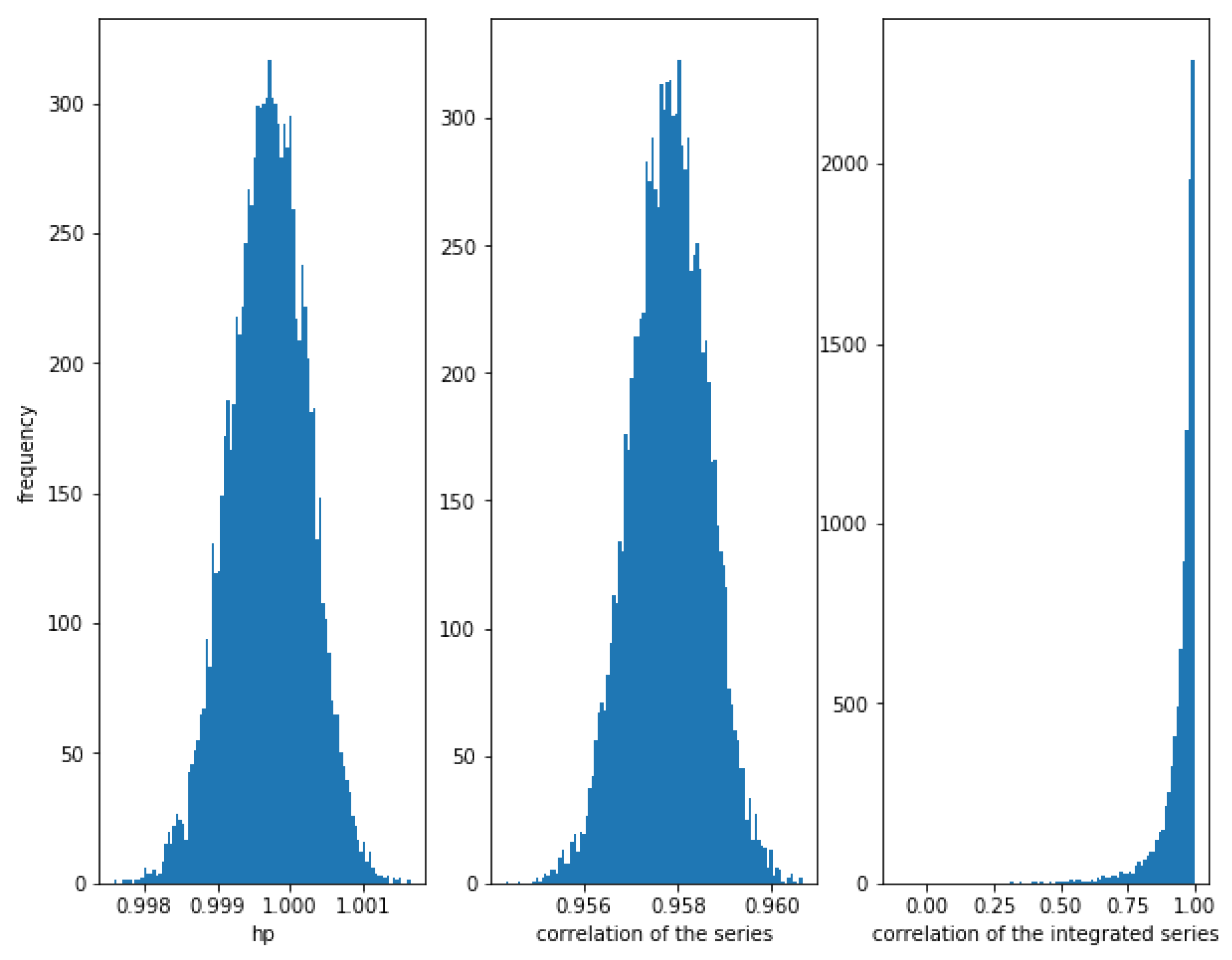
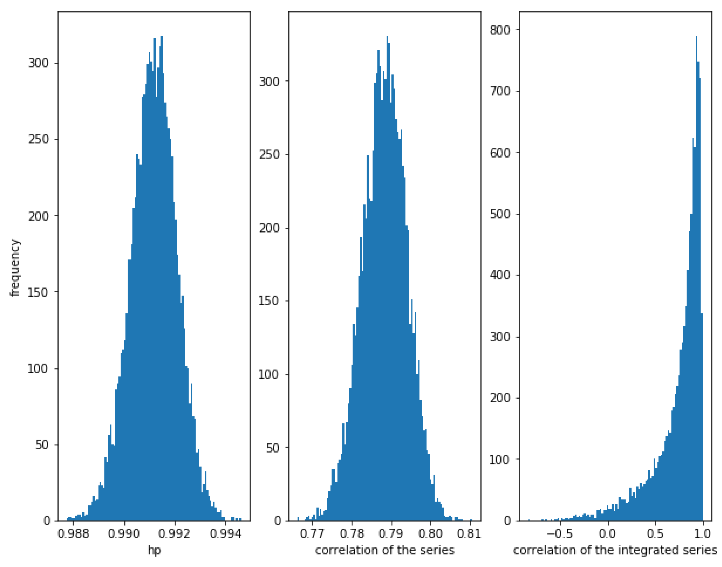
Consider two correlated series $x_t$ and $y_t=x_t+e_t$, where $x_t$ follows a Normal distribution $N(0,1)$ and $e_t$ follows an independent Normal distribution $N(0,\sigma )$. The smaller the value of $\sigma$, the greater the correlation. For example for $\sigma =0.3$ we can see in Figure 1, that the correlation between the series is high (close to 1), the correlation between the integrated series is also high (close to 1), and the HP of the series is also high (close to 1). Please note that the theoretical value of the correlation of the series and the correlation of the integrated series is $\frac{1}{\sqrt{1+{\sigma }^2}}\approx 0.96$.

Figure 1 shows the histogram of the correlation between the series, the integrated series as well as the HP of the series for 10,000 simulations of correlated series $x_t$ and $y_t$ as described previously, with a length of 10,000. Please note that the correlation of the integrated series shows a wider dispersion than the correlation of the series itself.

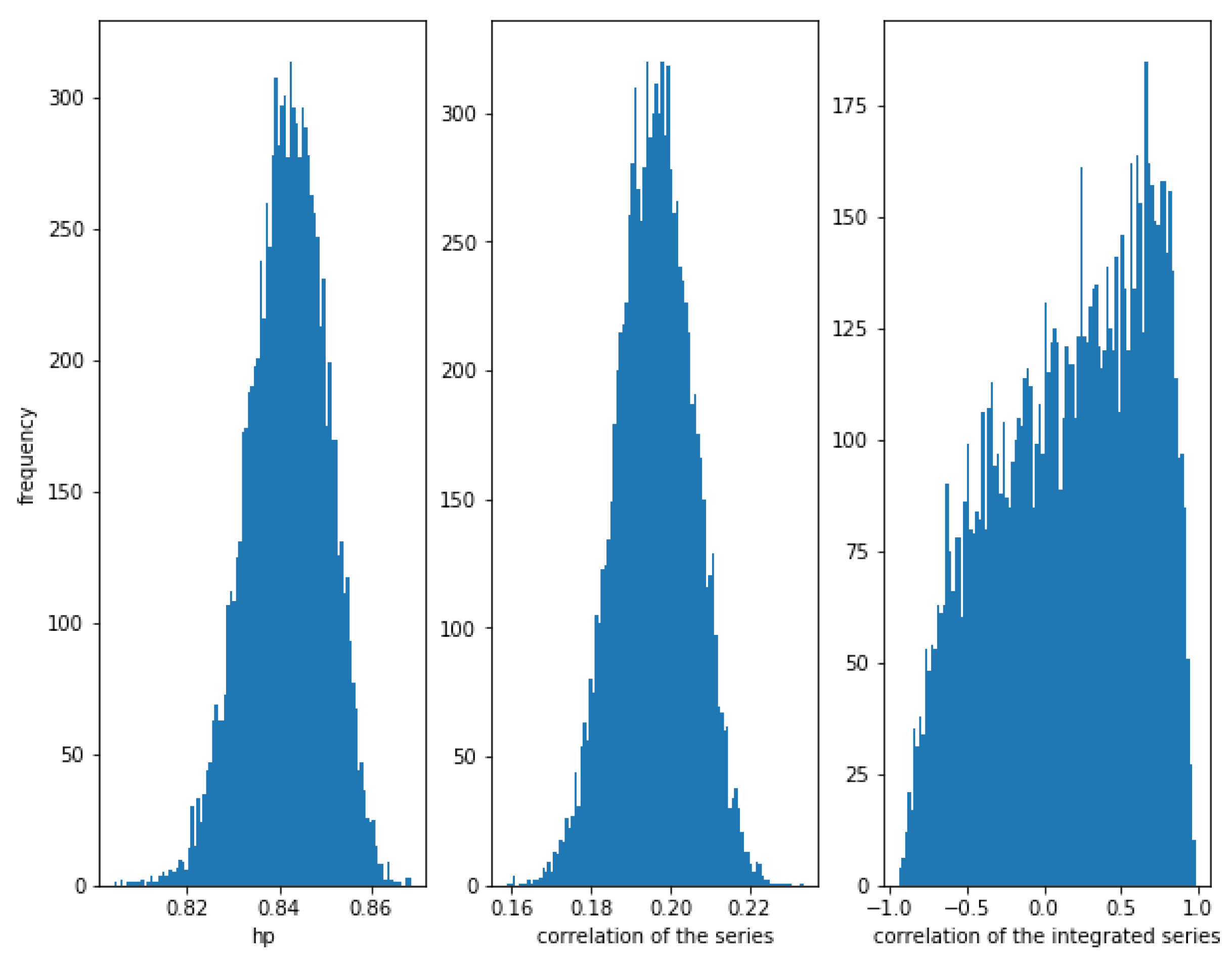
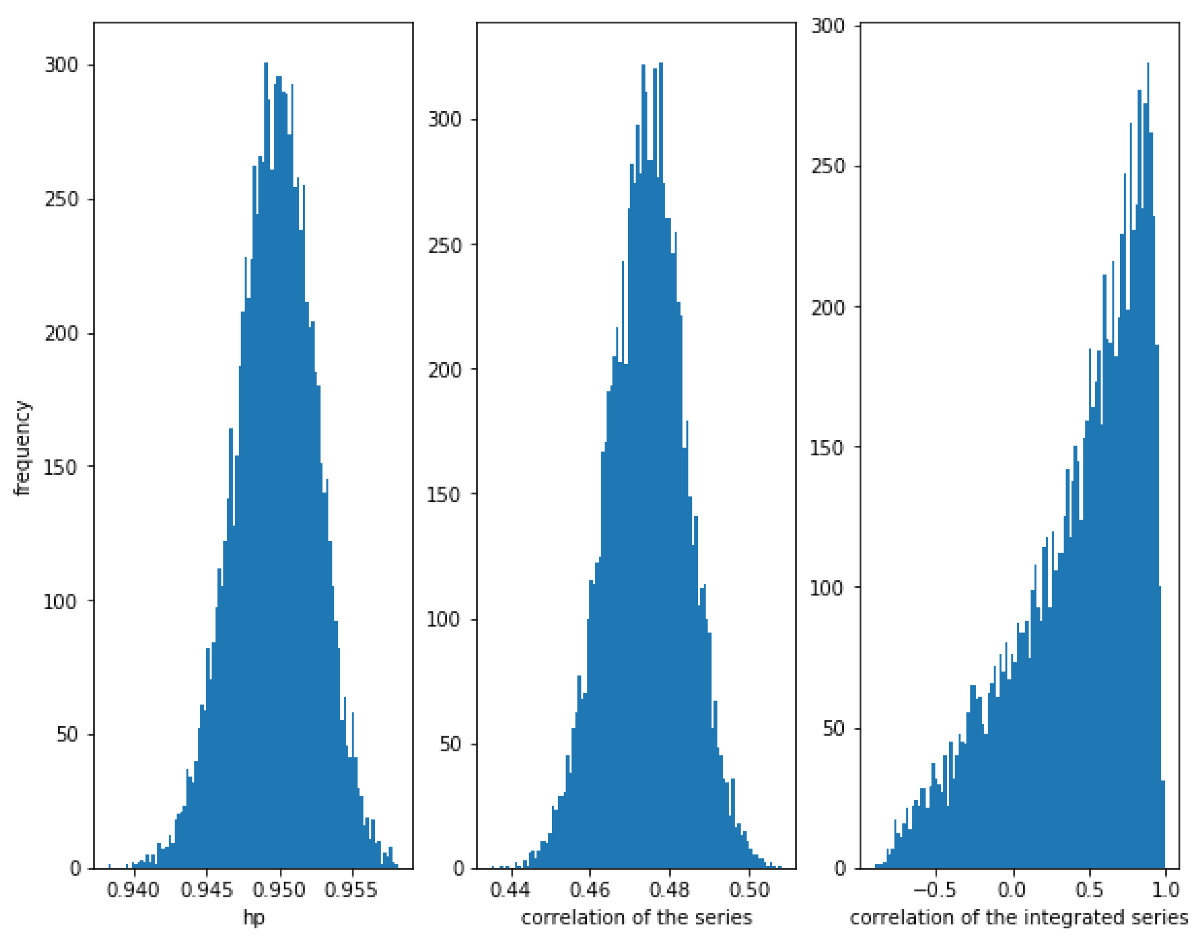
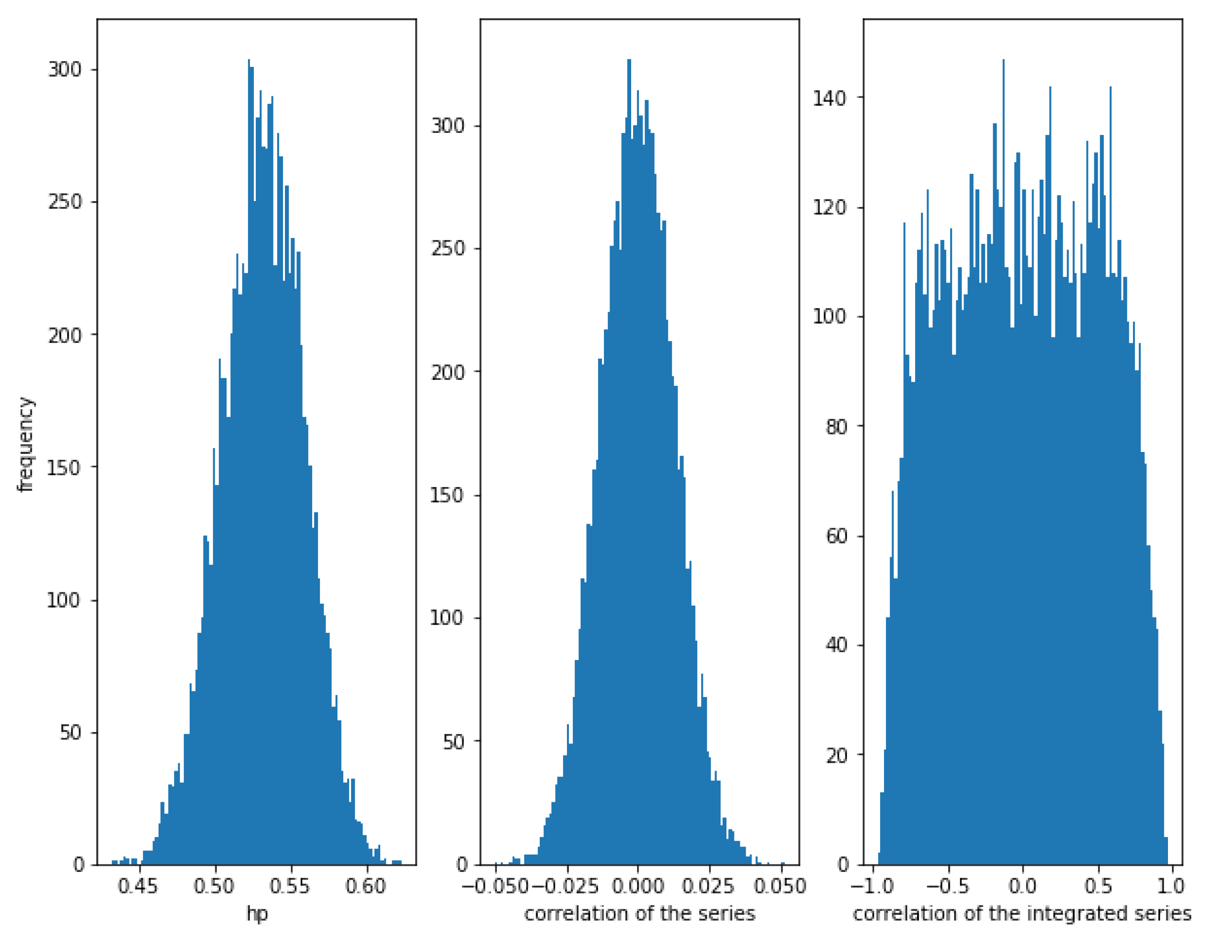
For $\sigma =5$, the correlation between the series is weaker (≈0.19), though there is a relationship between them. The correlations of the series and the integrated series are quite low (around the theoretical value), while the HP of the series is high (around $0.84$).

In Figure 2 can be observed again that the dispersion of the correlation of the integrated series is huge.

2.2.2. Cointegrated Series

Let $x_t$ follows a Normal distribution $N(0,1)$ and consider the series $z_n={\sum }_{i=0}^n{x}_t+e_t$, where $e_t$ follows a Normal distribution $N(0,\sigma )$. Let $y_t=z_{t+1}-z_t$. Then the integrated series of $x_t$ and $y_t$ are cointegrated. The lower the value of $\sigma$ the greater the relationship between the two series.

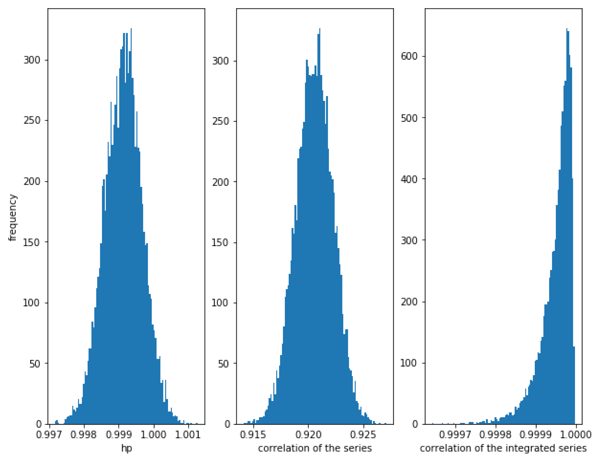
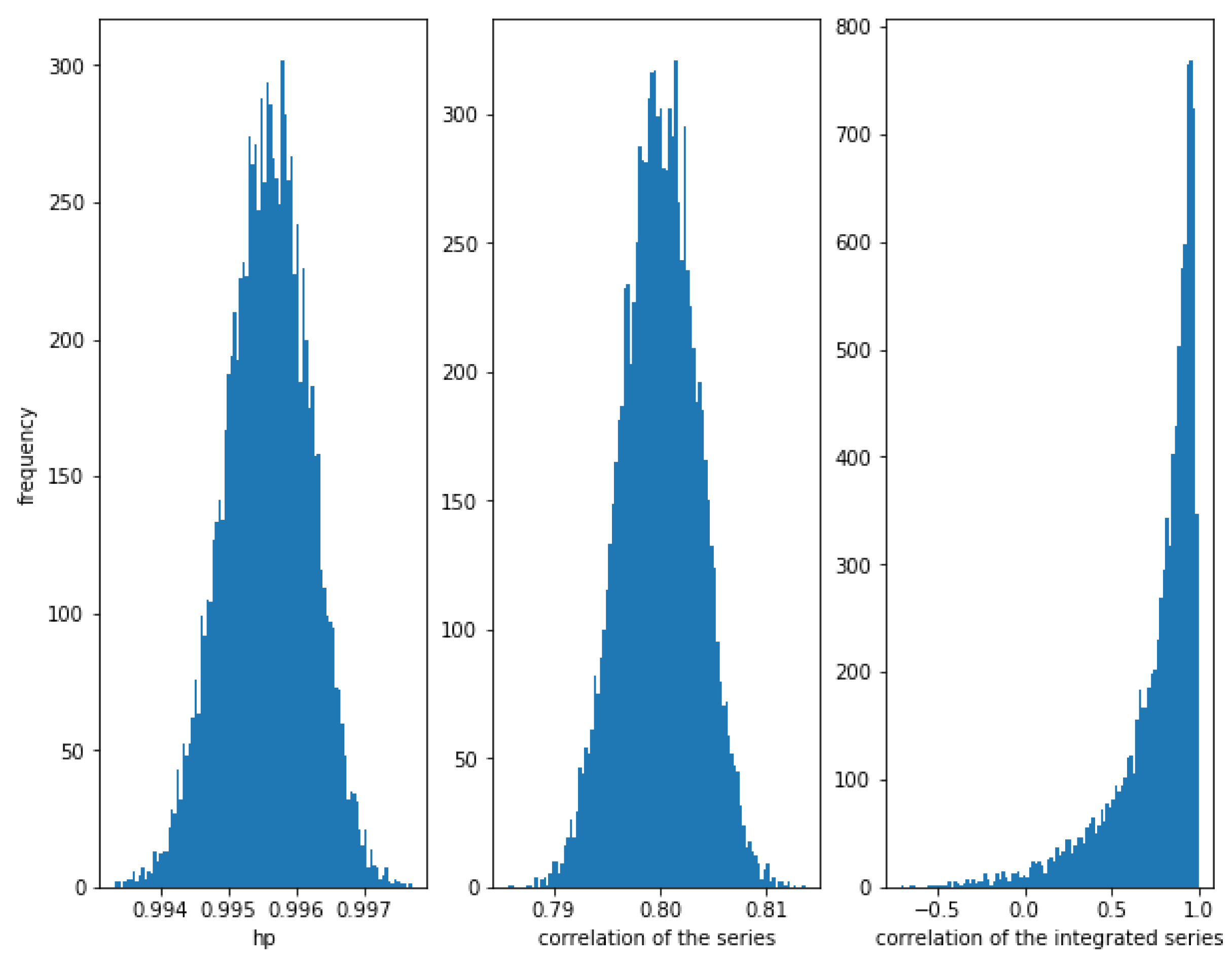
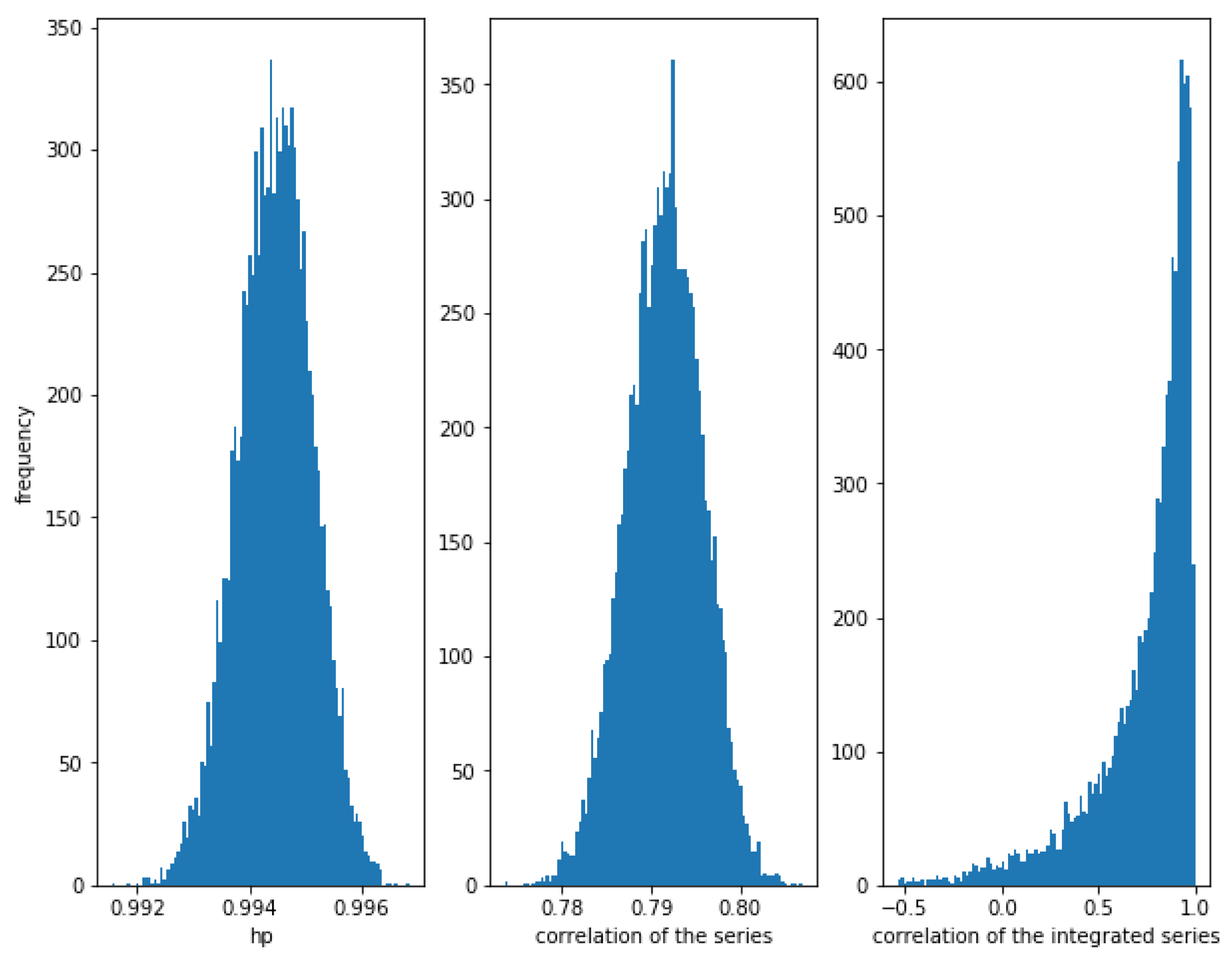
Figure 3 shows how for small values of $\sigma$ (in this case, $\sigma =0.3$), the correlation of the series and the integrated series as well as the HP of the series is very high.

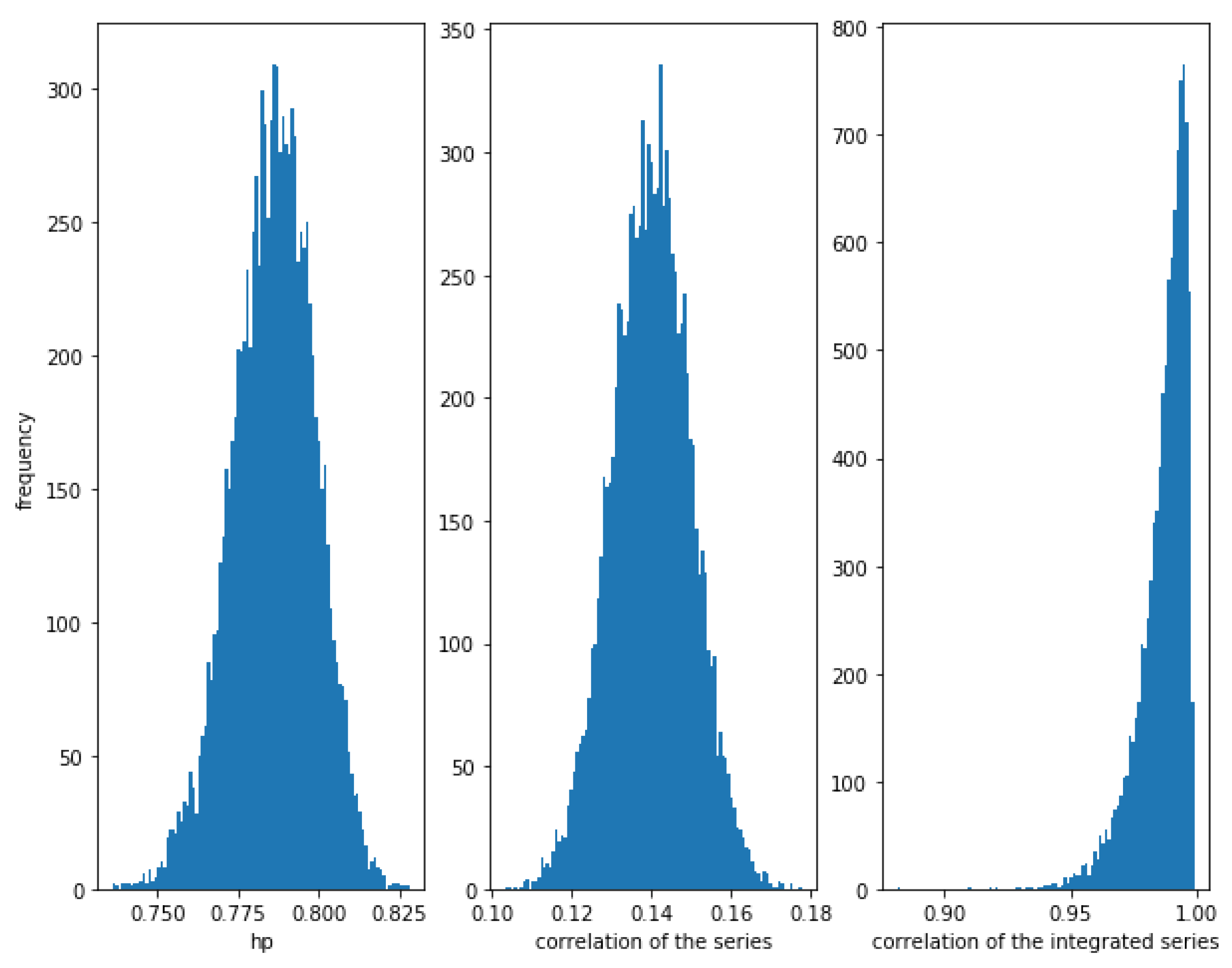
On the other hand, Figure 4 shows that when the noise is greater, i.e., for a greater value of $\sigma$ (in this case $\sigma =5$), the correlation between the series is weaker (≈0.14), though there is a relationship between them. The correlation of the integrated series is, as expected, very high with a narrow dispersion, in this case. The HP of the series is high (around $0.79$). Therefore, again, the HP is able to detect a relationship in the series.

2.2.3. Uncorrelated Series

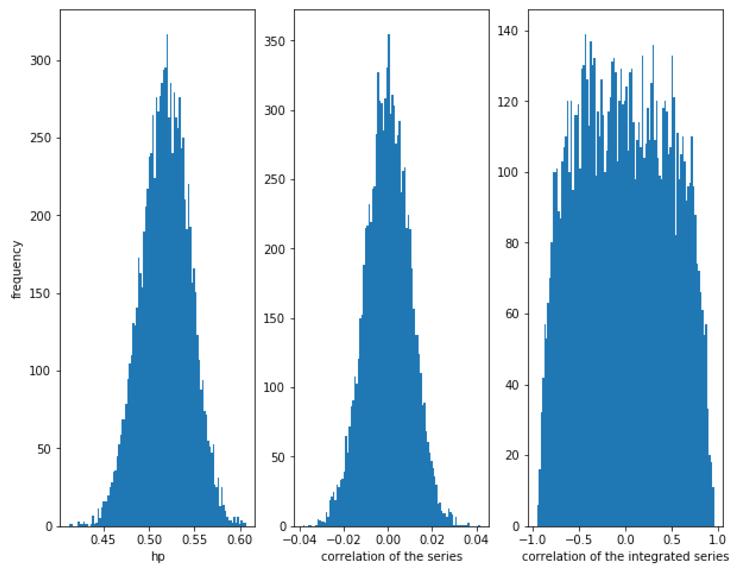
In the case of two independent series, Figure 5 shows how the HP is close to $0.5$, while the correlation of the series and the integrated series is close to 0, though the dispersion of the correlation of the integrated series is very high.

2.2.4. Nonlinear Relationship

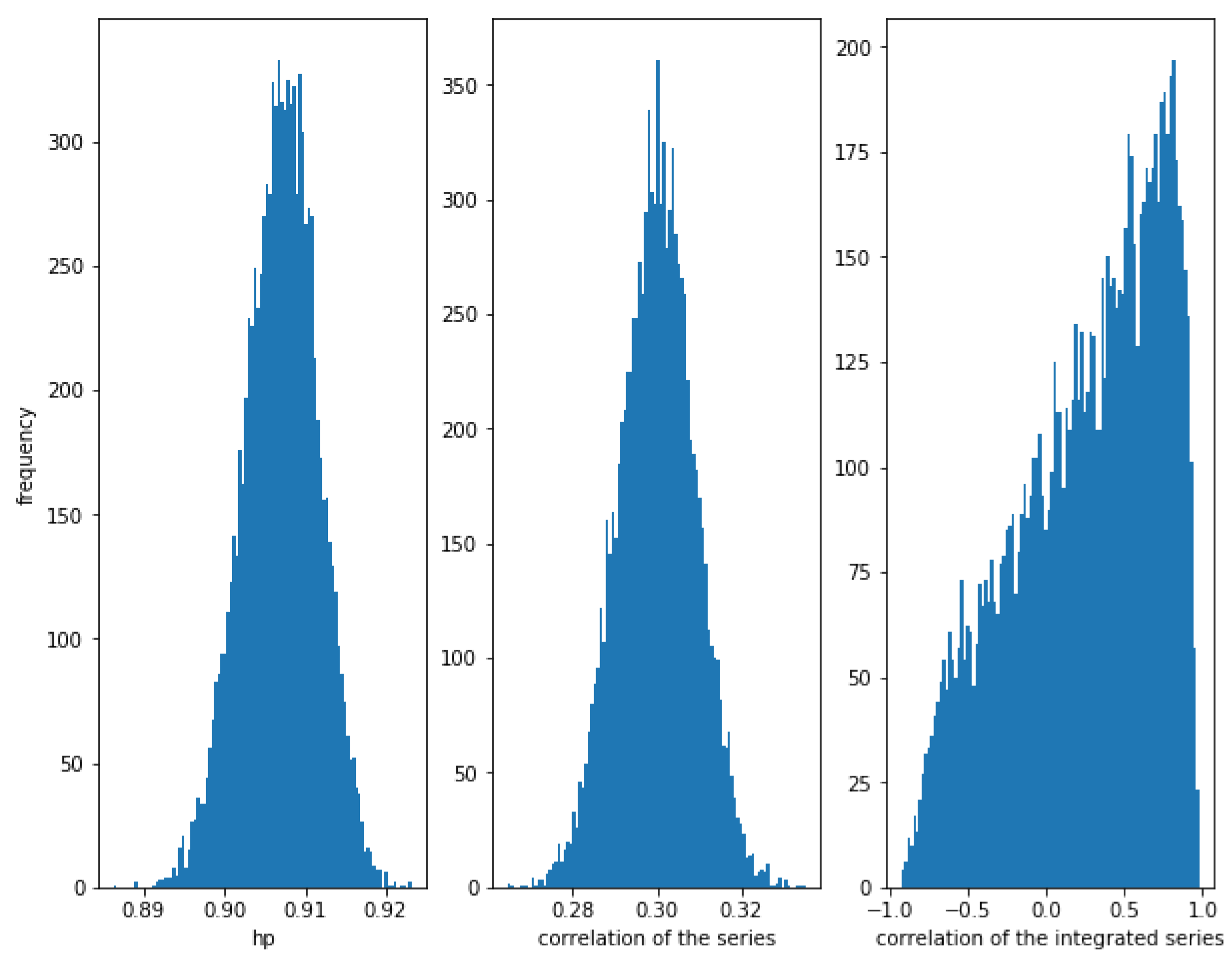
Consider the series $y_t=x_t^3+e_t$, where $x_t$ follows a Normal distribution $N(0,1)$ and $e_t$ follows an independent Normal distribution $N(0,\sigma )$. It is clear that there is a relationship between the series $x_t$ and $y_t$, but it is a non-linear relationship. In Figure 6, it can be observed that the HP of the series is very high (around $0.95$), while the correlation of the series and the integrated series is less than $0.5$. Please note that the dispersion of the correlation of the integrated series is very high, again.

2.2.5. Copula Relationship

Embrechts et al. [51] was the seminal paper where the concept of copula was introduced in finance. After this work, copula-based models were widely used in finance (for an interesting survey see Ass [52]). The main advantages of copula models are the possibility of modeling the multivariate dependence structure of assets, independently of the marginal distributions and a better consideration of the classic tail dependence.

The case of bivariate models is well known, but the case of higher dimension ones presents more problems. With the objective of improving the accuracy of parameters estimation, novel approaches were introduced, the most promising being the Pair-Copula Construction (PCC) [53,54,55]. Three of the most common copulae are the Gaussian, the Student’s t and the Gumbel copula. Ass et al. [56] shows that these copulae are able to catch the tail dependence of financial data. For a deeper discussion on the copulae described next, the reader is referred to [57]. In this section we will show that HP performances properly in the case of these copula models.

The Gaussian copula relationship case.

Consider a bivariate normal distribution with zero mean $\mu =(0,0)$ and covariance matrix $\Sigma =\left(\begin{array}{cc}1& \rho \\ \rho & 1\end{array}\right)$.

Please note that this distribution can be also described as a distribution with a Gaussian copula and standard normal marginal distributions $N(0,1)$.

For this distribution, the probability density function is given by

$$f(x,y)=\frac{1}{2\pi \sqrt{1-{\rho }^2}}exp\left(-\frac{1}{2(1-{\rho }^2)}(x^2+y^2-2\rho xy)\right)$$

Let $(x_n,y_n)$ be a sample of this distribution. First consider a high correlation $\rho =0.8$. In Figure 7, it can be observed that the HP of the series is very close to one, the correlation of the series is around $0.8$ as expected and the correlation of the integrated series is high, but with some dispersion.

Now, consider a weaker correlation $\rho =0.3$. In Figure 8, it can be observed that the HP of the series is still high (around $0.91$), while the correlation of the series is around $0.3$ as expected and the correlation of the integrated series has a lot of dispersion. We conclude that the HP method is able to detect this kind of relationship, even when the correlation is low.

The Student’s t copula relationship case.

Student’s t copula is derived from Student’s t bivariate distribution. For parameters $\nu >0$ degrees of freedom, mean vector $\mu =(0,0)\in {\mathbb{R}}^2$ and scale parameter matrix $\Sigma =\left(\begin{array}{cc}1& \rho \\ \rho & 1\end{array}\right)$ (note that $\Sigma$ is the correlation matrix for $\nu >2$), the bivariate standard Student’s t density function is given by

$$t(x,y)=\frac{\Gamma \left(\frac{\nu +2}{2}\right){(1-{\rho }^2)}^{-\frac{1}{2}}}{\Gamma \left(\frac{\nu }{2}\right)\nu \pi }{\left(1+\frac{1}{\nu }\frac{x^2+y^2-2\rho xy}{1-{\rho }^2}\right)}^{-\frac{\nu +2}{2}}$$

Now, if T is the cumulative distribution function of the bivariate standard Student’s t distribution and $T_{\nu }$ is the cumulative distribution function of the univariate Student’s t distribution with $\nu$ degrees of freedom, then, by Sklar’s Theorem, the Student’s t copula of parameters $\nu$ and $\Sigma$ is given by

$$C_T(u,v)=T(T_{\nu }^{-1}\left(u\right),T_{\nu }^{-1}\left(v\right))$$

Finally, consider a distribution given by the Student’s t copula of parameters $\nu$ and $\Sigma =\left(\begin{array}{cc}1& \rho \\ \rho & 1\end{array}\right)$ and standard normal marginal distributions $N(0,1)$. By Sklar’s Theorem, its bivariate cumulative distribution function is given by $F(x,y)=C_T(F_N\left(x\right),F_N\left(y\right))$, where $C_T$ is the Student’s t copula and $F_N$ is the cumulative distribution function of a standard normal distribution.

Let $(x_n,y_n)$ be a sample of this distribution. First consider a high correlation $\rho =0.8$ and $\nu =3$. In Figure 9, it can be observed that the HP of the series is very close to one, the correlation of the series is around $0.79$ and the correlation of the integrated series is high, but with some dispersion.

Now, consider a weaker correlation $\rho =0.3$ and $\nu =3$. In Figure 10, it can be observed that the HP of the series is still high (around $0.88$), while the correlation of the series is around $0.29$ and the correlation of the integrated series has a lot of dispersion. We conclude that the HP method is able to detect this kind of relationship, even when the correlation is low.

Finally, consider the case for $\rho =0$ and $\nu =3$. In this case, there is no correlation in the series (since $\rho =0$), but the Student’s copula with these parameters is not the independent copula, so there is some (very slight) kind of dependence between the series (for example, upper and lower tail dependence). In this case the mean of the HP of the series is about $0.531$ (with a standard deviation of $0.027$) while for independent series the mean of the HP of the series is about $0.518$ (with a standard deviation of $0.027$). The difference is so small that it cannot be say that HP is able to detect this subtle dependence. In Figure 11, it can be observed that the HP of the series is around $0.53$, the correlation is around 0, as expected, as well as the correlation of the integrated series, but with a huge dispersion in the latter case.

The Gumbel copula relationship case.

The Gumbel copula is an Archimedean copula given by

$$C(u,v)=exp\left(-{({(-log(u))}^{\theta }+{(-log(v))}^{\theta })}^{\frac{1}{\theta }}\right)$$

where $\theta \in [1,\infty ]$ is the parameter of the copula and $u,v\in [0,1]$.

Let $(x_n,y_n)$ be a sample of a distribution given by the Gumbel copula and standard normal marginal distributions $N(0,1)$. By Sklar’s Theorem, its bivariate cumulative distribution function is given by $F(x,y)=C(F_N\left(x\right),F_N\left(y\right))$, where C is the Gumbel copula described previously (of parameter $\theta$) and $F_N$ is the cumulative distribution function of a standard normal distribution.

Please note that for the Gaussian and the Student’s t copula, the Kendall’s $\tau$ is equal to $\tau =\frac{2}{\pi }arcsin\rho$ and for the Gumbel copula $\tau =\frac{\theta -1}{\theta }$, so a Gumbel copula with $\theta =\frac{1}{1-\frac{2}{\pi }arcsin\left(\rho \right)}$ will have the same Kendall’s $\tau$ than a Gaussian and a Student’s t copula with parameter $\rho$. Hence, a Gumbel copula with $\theta \approx 2.44$ has the same Kendall’s $\tau$ than a Gaussian and a Student’s t copula with $\rho =0.8$ and a Gumbel copula with $\theta \approx 1.24$ has the same Kendall’s $\tau$ than a Gaussian and a Student’s t copula with $\rho =0.3$.

First, consider a high relationship between $x_n$ and $y_n$ with $\theta =2.44$. In Figure 12, it can be observed that HP is very high (around $0.995$) and the correlation of the series is quite high (around $0.79$). The correlation of the integrated series is often high but there is quite dispersion.

Now, consider a weaker relationship with $\theta =1.24$. In Figure 13, it can be observed that the HP of the series is still high (around $0.9$), while the correlation of the series is much weaker (around $0.31$) and the correlation of the integrated series has a lot of dispersion. We conclude, again, that the HP method is able to detect this kind of relationship, even when the correlation is low.

As a consequence of the previous analyses, it can be concluded that the HP of two series is able to detect a relationship between them, of course when this relationship is correlation, but also when it is cointegration or even for a non-linear one or when the relationship is more complex and given by a copula. Furthermore, for two stocks, the HP will be high even if most of the time there is no correlation between its returns, but the correlation appears when the absolute value of the returns are high. We will explore the HP of two stocks in the next section.

3. Testing HP in Financial Series

In this section, the application of the HP is explored to measure the relationship between two financial series. First, the co-movement of a pair of ETFs is analyzed when there is a strong relationship and when the relationship is weaker. Then, this new method will be applied in a statistical arbitrage strategy.

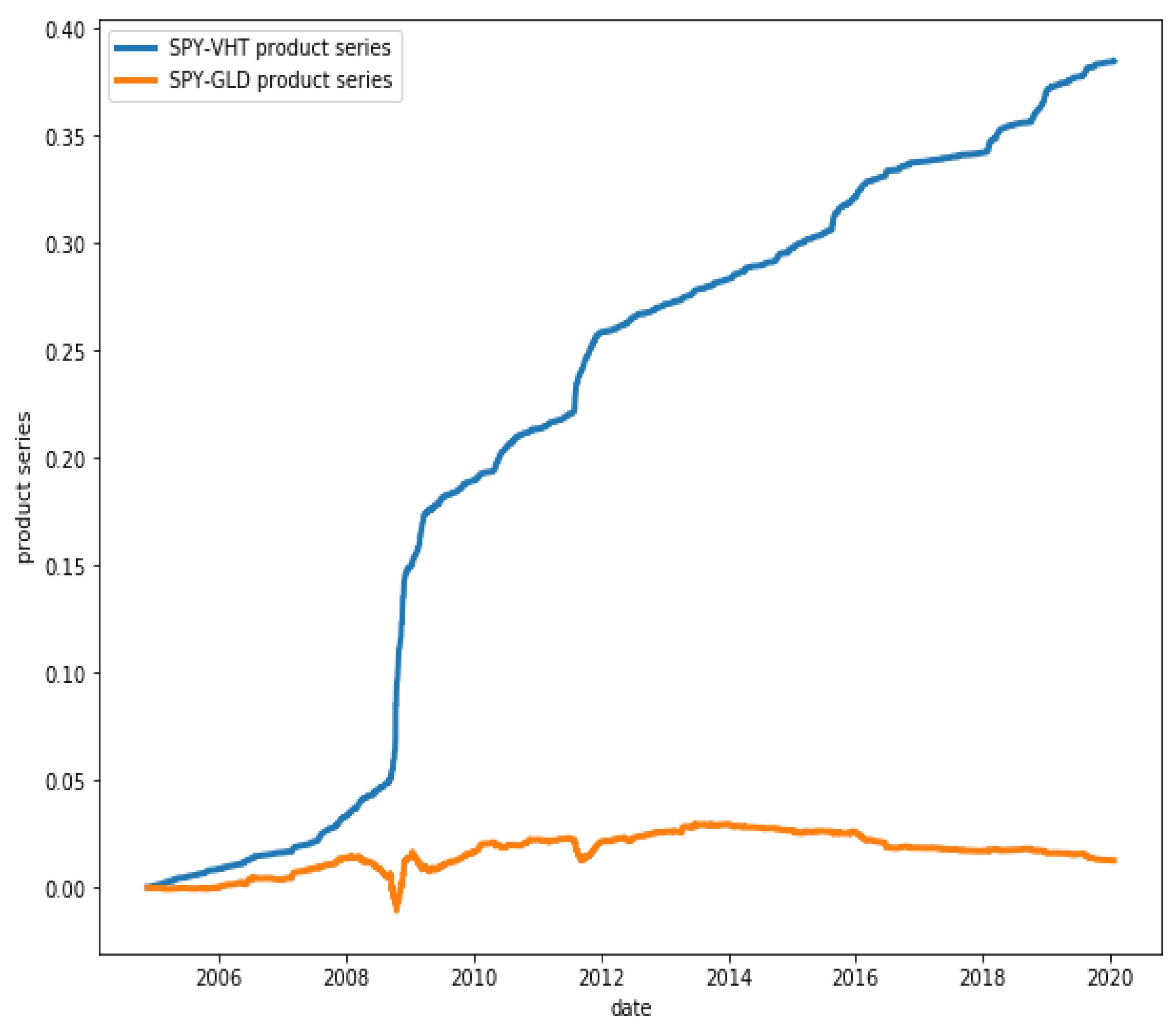
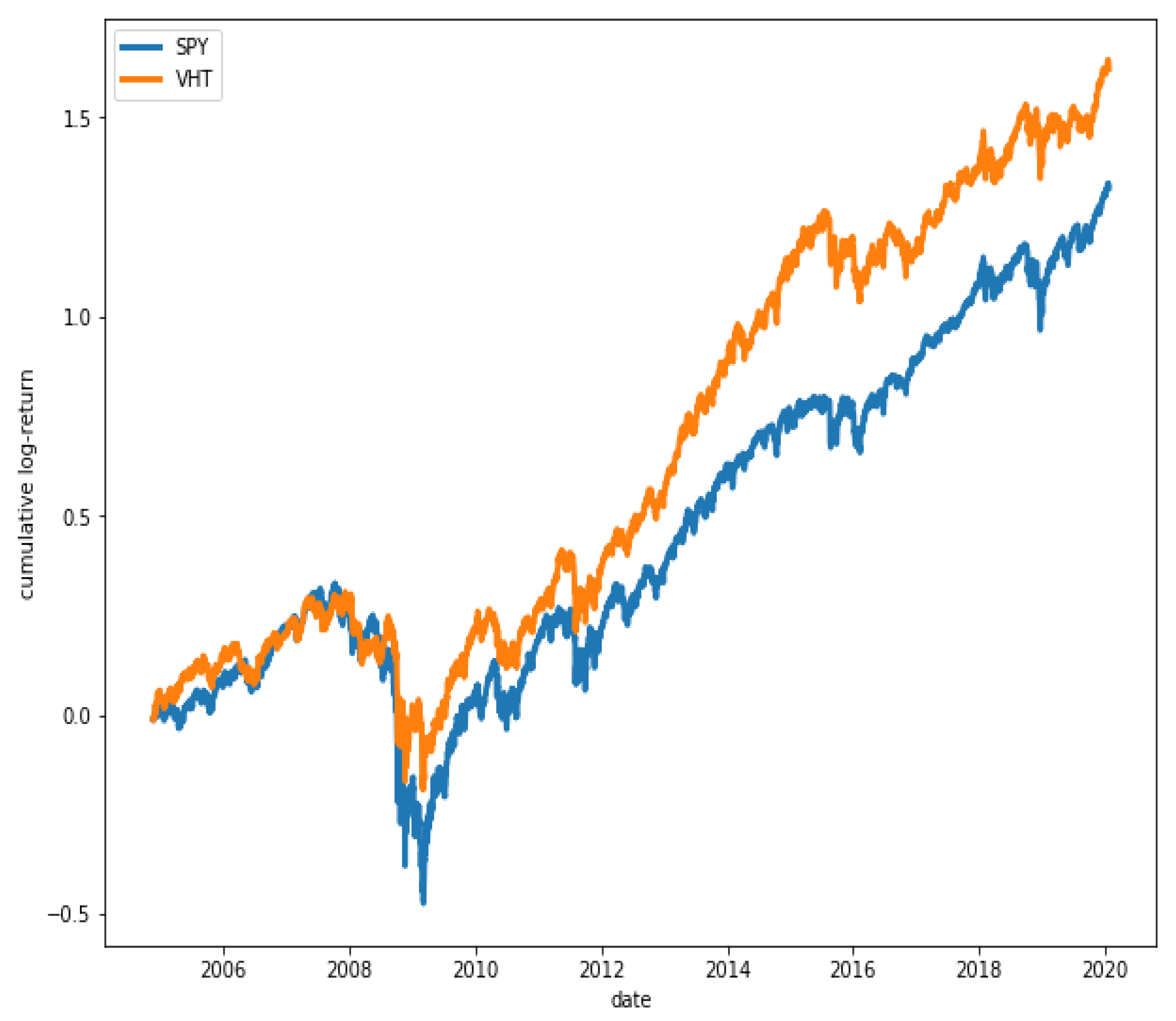
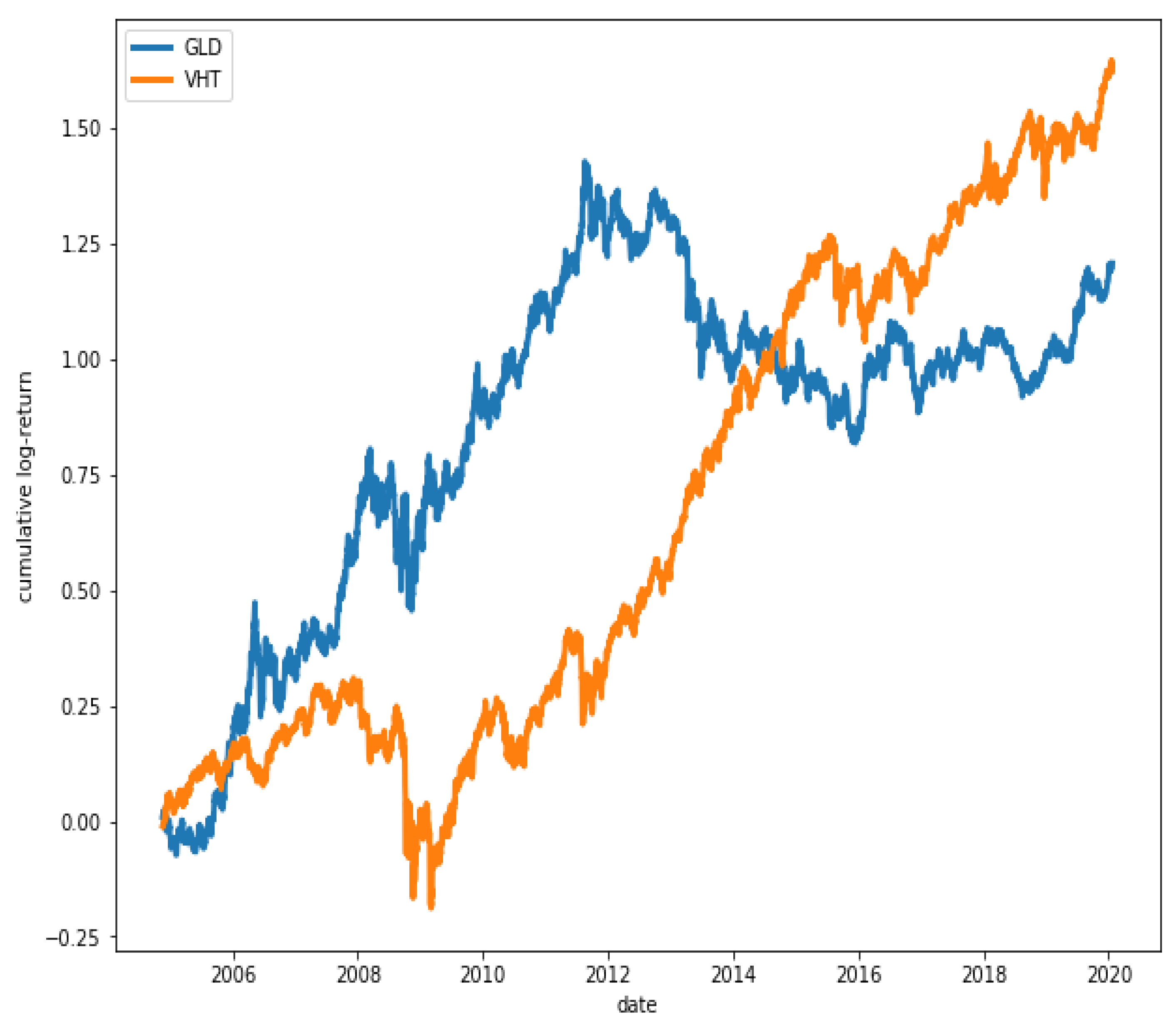
Figure 14 presents two series: the blue one is for the product series of the returns of the ETFs SPY (SPDR S&P 500 ETF Trust) and VHT (Vanguard Health Care ETF), which have HP $=0.998$, while the orange one is for the product series of the returns of the ETFs GLD (SPDR Gold Trust) and VHT, which have a much weaker co-movement with HP $=0.691$.

Figure 15 shows that ETFs SPY and VHT have, in fact, a great degree of co-movement, while in Figure 16, it is observed that ETFs GLD and VHT have a much lower degree of co-movement, as expected.

3.1. Paris Trading: Strategy Definition and Application

HP will be tested through a statistical arbitrage technique known as Pairs Trading, which consists of looking for two shares whose historical prices have moved in a similar way and arbitrate them when there is a deviation between them [58]. This strategy was born in a North American investment bank in the 1980s [59]. In the scientific field, many studies were developed in which different selection methods were introduced, from the simplest ones such as the method of distance [60] or correlation, to more complex methods, such as cointegration [59], copula [61] or the Hurst exponent [62].

As it was explained in Section 2.2, the HP model is proposed as an alternative to correlation, which is why in this section a comparison using both models is done, to check whether it is true that our model is superior to the correlation method. In a previous work [62], it is shown that the strategy of Pairs Trading does not obtain good results by selecting those highly correlated pairs. The goal of this section is to test if a Pairs Trading strategy based on HP improves the performance of the strategy.

Since in a Pairs Trading strategy we look for two assets with a high degree of co-movement, we can search a pair of assets with a high value of HP (close to 1). On the other hand, note that if the returns are small, it is not so important that the two assets move in the same direction as when the returns are greater. This method takes this into consideration.

The trading strategy is as follows:

• First, the prices are normalized as defined by Ramos-Requena et al. (2017) [62]. Therefore, for a pair of stocks A and B, for each dollar invested in A we will invest b dollars in B, where b is given by $b=std\left(r_A\right)/std\left(r_B\right)$, and $r_A$ (resp. $r_B$) is the log-return of A (resp. B).
  The series of the pair is defined such that its increments are given by $r_A-b{r}_B$.
• Pairs selection:
  To select the pairs, the correlation method is chosen by using Pearson’s correlation method and through the HP method, as it was explained in Section 2.2. The duration of this phase will be 250 or 500 days, as we will indicate later.
• Trading strategy (see Ramos-Requena et al. (2017) [62] for a more detailed description):
  • When $s>m+\sigma$ the pair is sold. The position is closed when $s<m$ or $s>m+2\sigma$.
  • When $s<m-\sigma$ the pair is bought. The position is closed when $s>m$ or $s<m-2\sigma$.
  where m is a moving average of the series of the pair and s is a moving standard deviation of m.

The duration of this phase is 120 days.

The results obtained will be divided into three subsections:

• HP: daily returns are used.
• HP1: 10 days (2 weeks) returns are chosen.
• HP2: 20 days (4 weeks) returns are chosen and the selection period is 500 days (around 2 years).

In any case, the stocks of the Dow Jones index are used, for the period 2000–2018, with transaction costs of 0.01% per trade.

3.2. HP

Table 1. Results obtained for the period 2000–2018, where N is the number of pairs; AAV is the average annualized return; Sharpe R is the Sharpe Ratio and Profit is the profitability for the full period with transaction costs.

Method	N	AAV	Sharpe R	% Max Drawdonw	% Profit
Correlation	2	0.50%	0.12	12.30%	6.20%
HP	2	0.30%	0.05	13.40%	1.20%
Correlation	5	0.30%	0.70	18.30%	1.27%
HP	5	1.00%	0.28	9.40%	16.30%
Correlation	10	0.00%	−0.01	9.80%	−4.41%
HP	10	0.20%	0.07	10.90%	−0.04%
Correlation	15	0.00%	−0.01	10.90%	−4.25%
HP	15	0.60%	0.22	6.80%	6.80%
Correlation	20	0.00%	0.02	7.40%	−2.93%
HP	20	0.20%	0.08	7.00%	−0.52%
Correlation	25	0.60%	0.27	5.30%	6.86%
HP	25	0.30%	0.12	6.70%	1.00%
Correlation	30	0.40%	0.18	5.60%	2.75%
HP	30	0.00%	0.00	6.80%	−3.70%

presents the main results obtained for HP.

As shown in the table, the highest return is achieved for the portfolio composed of 5 pairs, selecting them through the HP method (16.30%). It is significant that for the 15 pairs portfolio the return obtained through the HP is 6.8% while the correlation obtains a negative return of −4.25%. Analyzing the annualized profitability, it can be observed that the best result is obtained for the portfolio composed by 5 pairs (1%). Finally, the Sharpe ratio shows that the highest return per unit of risk is obtained for the portfolio of 5 pairs by selecting them through correlation.

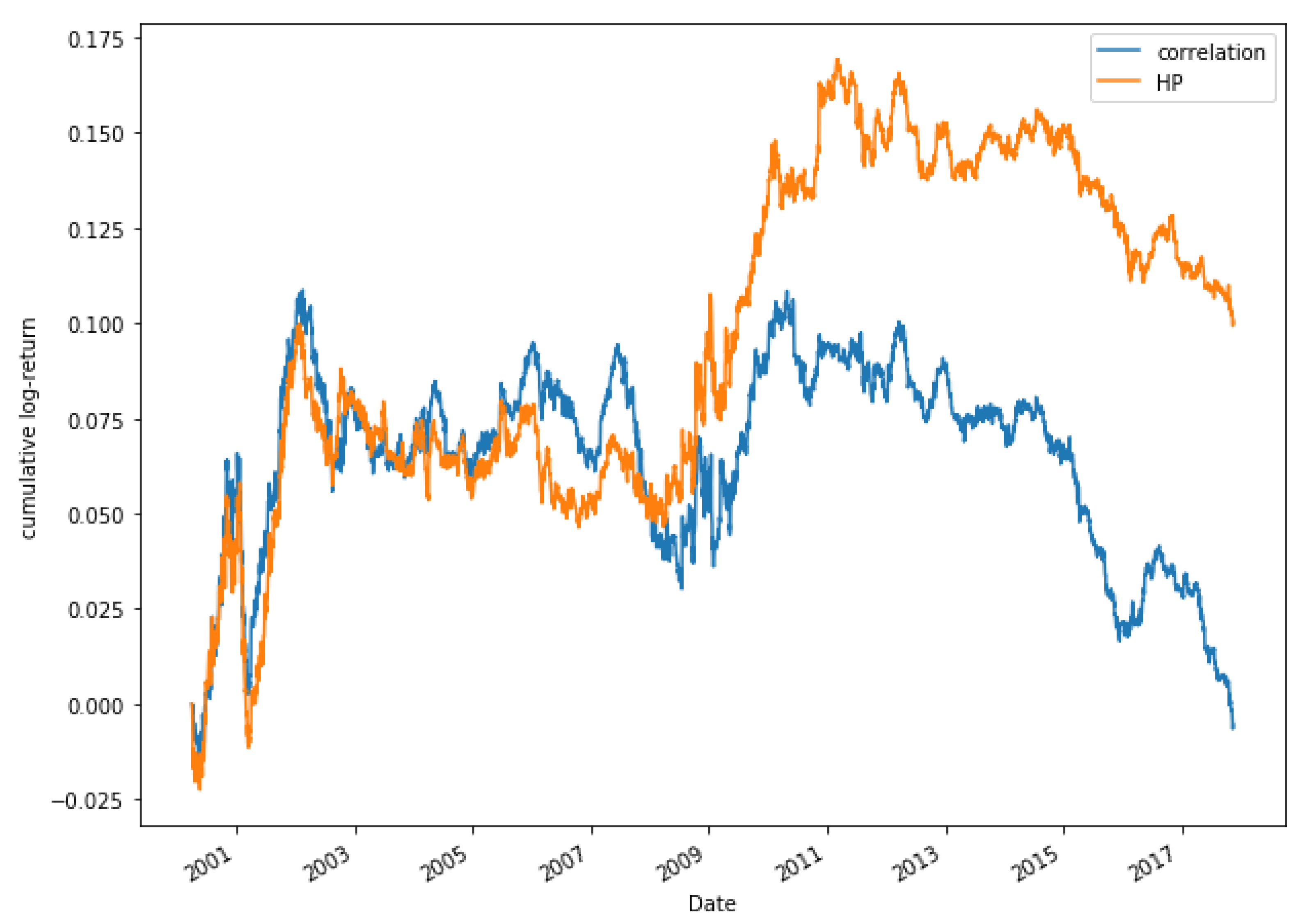
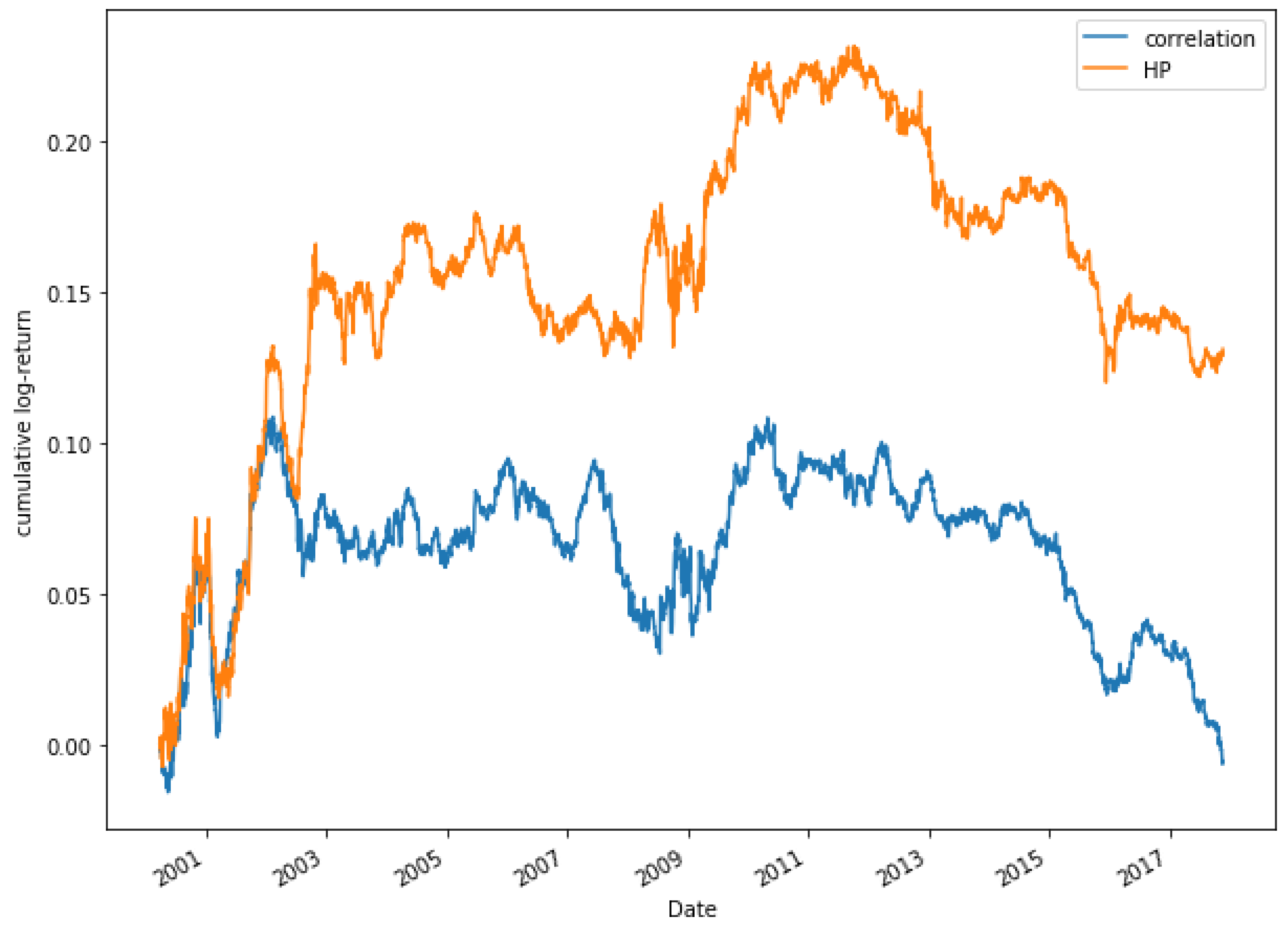
Figure 17 shows a comparison between the correlation method and HP for the period 2000 to 2018 for a portfolio consisting of 15 pairs. It can be appreciated that both models moves similarly until 2009. From 2009 there is a much higher increase in the returns obtained by the HP method. Figure 18 shows the returns obtained for the portfolio made up of 20 pairs. For this portfolio, the results obtained are very similar. During the period 2000–2009 the best option is to select the pairs through the correlation method. From 2010, the performance is higher through the HP method.

3.3. HP1

In this case, to calculate the HP of the series, it is used 10 days returns (instead of daily returns).

Table 2. Results obtained for the period 2000–2018, where N is the number of pairs; AAV is the average annualized return; Sharpe R is the Sharpe Ratio and Profit is the profitability for the full period with transaction costs.

Method	N	AAV	Sharpe R	% Max Drawdown	% Profit
Correlation	2	0.50%	0.12	12.30%	6.20%
HP1	2	0.80%	0.12	20.80%	11.32%
Correlation	5	0.30%	0.07	18.30%	1.27%
HP1	5	0.30%	0.07	18.30%	1.84%
Correlation	10	0.00%	−0.01	9.80%	−4.41%
HP1	10	0.50%	0.14	11.50%	5.22%
Correlation	15	0.00%	−0.01	10.90%	−4.25%
HP1	15	0.70%	0.25	10.60%	10.20%
Correlation	20	0.00%	0.02	7.40%	−2.93%
HP1	20	0.40%	0.16	9.80%	4.08%
Correlation	25	0.60%	0.27	5.30%	6.86%
HP1	25	0.30%	0.11	9.90%	1.01%
Correlation	30	0.40%	0.18	5.60%	2.75%
HP1	30	0.20%	0.09	8.90%	−0.20%

shows a comparison with the results obtained.

As Table 2 shows, in this case, for most portfolios (2, 5, 10, 15, and 20 pairs) the results obtained are better through the HP method than through correlation. It should be noted that for this period the best result is obtained for the portfolio composed of two pairs (11.32%). With respect to the average annualized profitability, it can be observed that for the case of the portfolio composed of 15 pairs, the difference between the models is 0.7%. With respect to the indicators that analyze the risk taken (Sharpe Ratio and Maximum Drawdown), the best results are obtained for the correlation model and the portfolio composed of 25 pairs with a Sharpe ratio of 0.27 and a maximum drawdown of 5.30%. If the sharpe ratio is considered, it is higher in most cases through the HP method, highlighting the portfolio with 15 pairs with a value of 0.25.

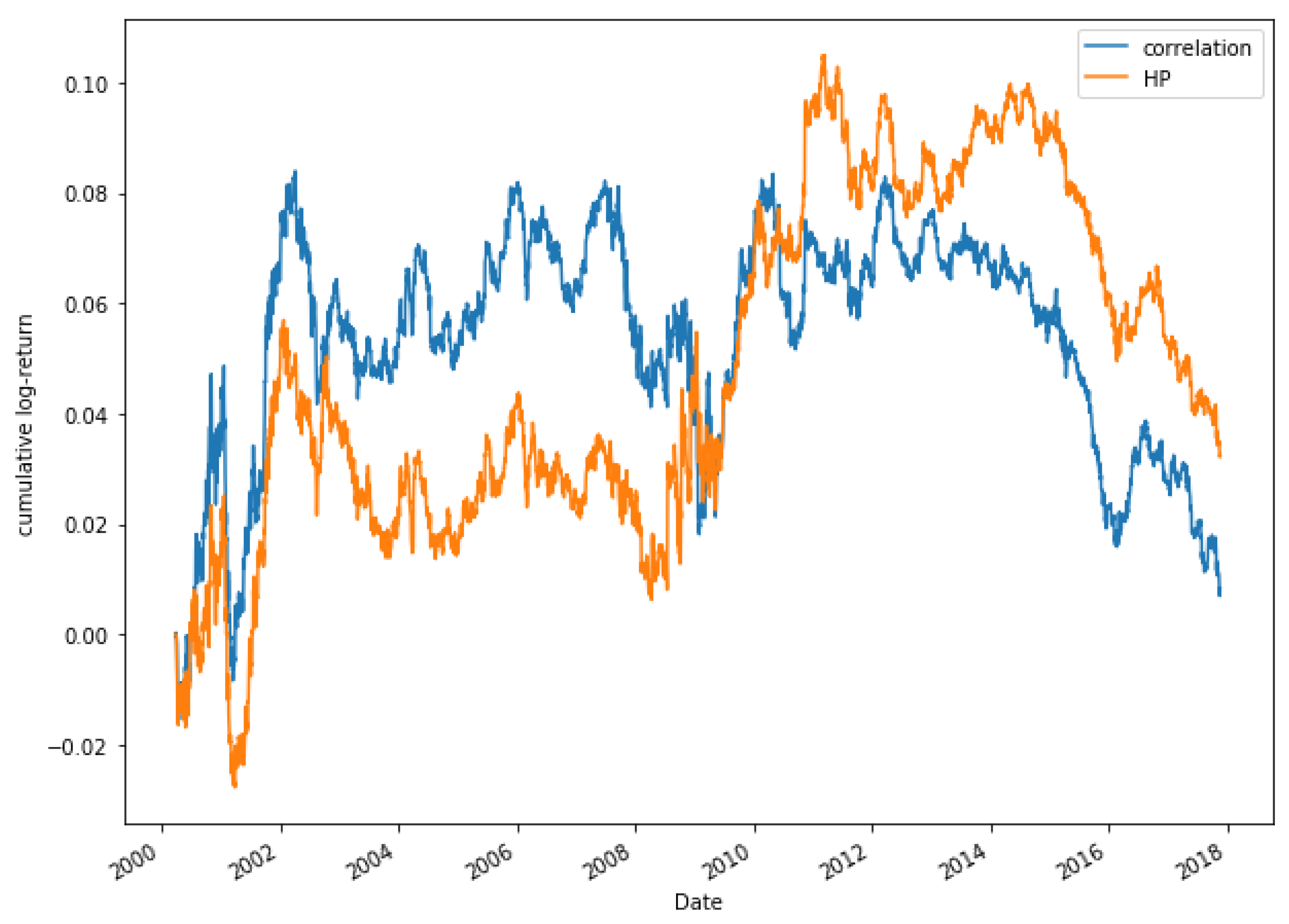
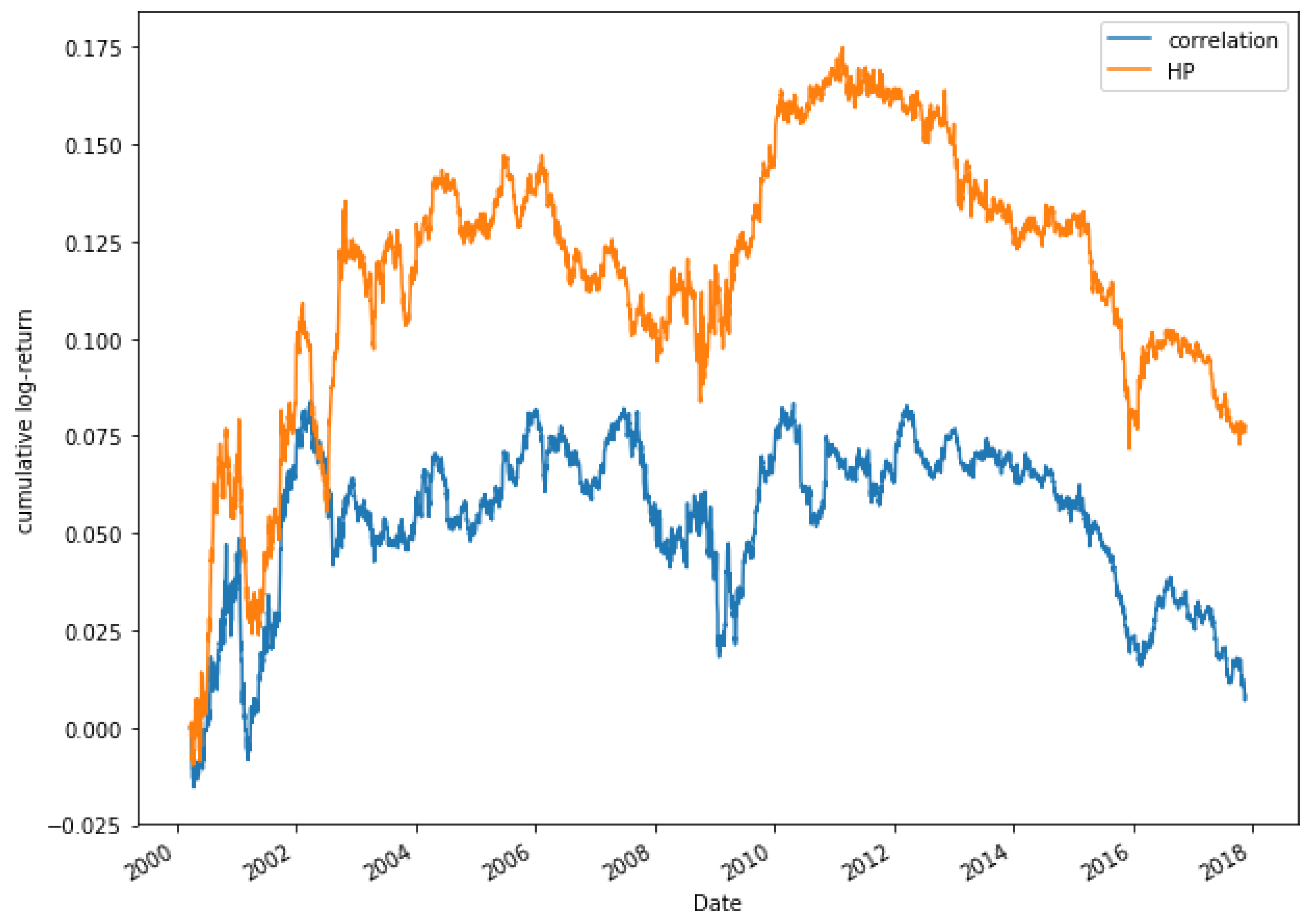
Figure 19 shows the comparison between the correlation and HP methods for a portfolio of 15 pairs. During the first years of study, it is observed that both models move in a very similar way. It is not until 2003 that the HP approach begins to grow, while the correlation method decreases, even obtaining negative returns. The comparison between models for a portfolio composed of 20 pairs is shown in Figure 20, where similar results to the case of 15 pairs are obtained.

3.4. HP2

For the HP2 method, to calculate the HP of the series it is used 20 days returns (instead of daily returns), and in this case the length of the selection period is increased to 500 days.

Table 3. Results obtained for the period 2000–2018, where N is the number of pairs; AAV is the average annualized return; Sharpe R is the Sharpe Ratio and Profit is the profitability for the full period with transaction costs.

Method	N	AAV	Sharpe R	% Max Drawdonw	% Profit
Correlation	2	−1.40%	−0.32	30.00%	−24.67%
HP2	2	1.20%	0.20	23.20%	19.64%
Correlation	5	1.10%	−0.32	23.10%	−20.71%
HP2	5	1.60%	0.39	15.00%	27.43%
Correlation	10	−0.80%	−0.28	15.10%	−15.54%
HP2	10	0.70%	0.23	13.00%	9.31%
Correlation	15	−0.30%	−0.11	12.10%	−7.74%
HP2	15	0.70%	0.26	7.50%	8.71%
Correlation	20	−0.30%	−0.15	13.00%	−8.83%
HP2	20	0.70%	0.31	6.20%	9.43%
Correlation	25	−0.40%	−0.19	12.50%	−9.76%
HP2	25	0.60%	0.29	5.10%	7.59%
Correlation	30	0.00%	0.00	10.70%	−3.54%
HP2	30	0.60%	0.30	5.80%	7.39%

presents the results obtained, considering transaction costs of 0.01%.

As Table 3 shows, the HP method obtains better results than the correlation one, which in this case obtains negative returns for all the portfolios studied. The highest return is achieved for the HP approach in the portfolio made up of five pairs (27.43%). With regard to the average annualized return, the same portfolio and model with an annualized return of 1.6% can be highlighted. Focusing on the Sharpe ratio, the best return per unit of risk is found for the portfolio of 5 pairs using the HP method with a value of 0.39. In the case of the correlation approach in most portfolios, it obtains a negative Sharpe ratio. Finally, looking at the data obtained in the maximum drawdown, the optimal portfolio is the one composed of 25 pairs, using the HP model, as it is the lowest value (5.10%), therefore, it is the minimum loss suffered by the portfolios studied for the period 2000–2018.

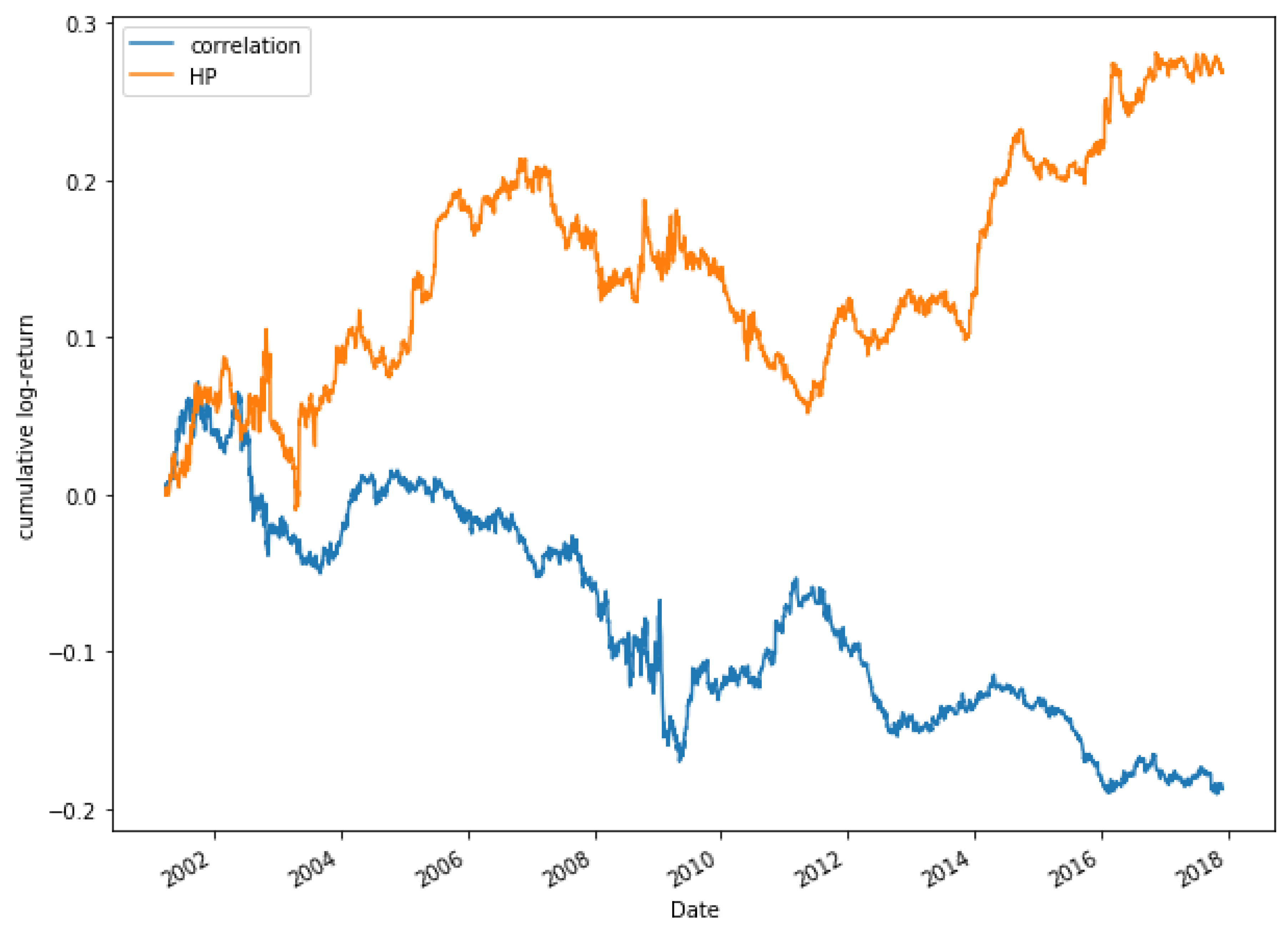
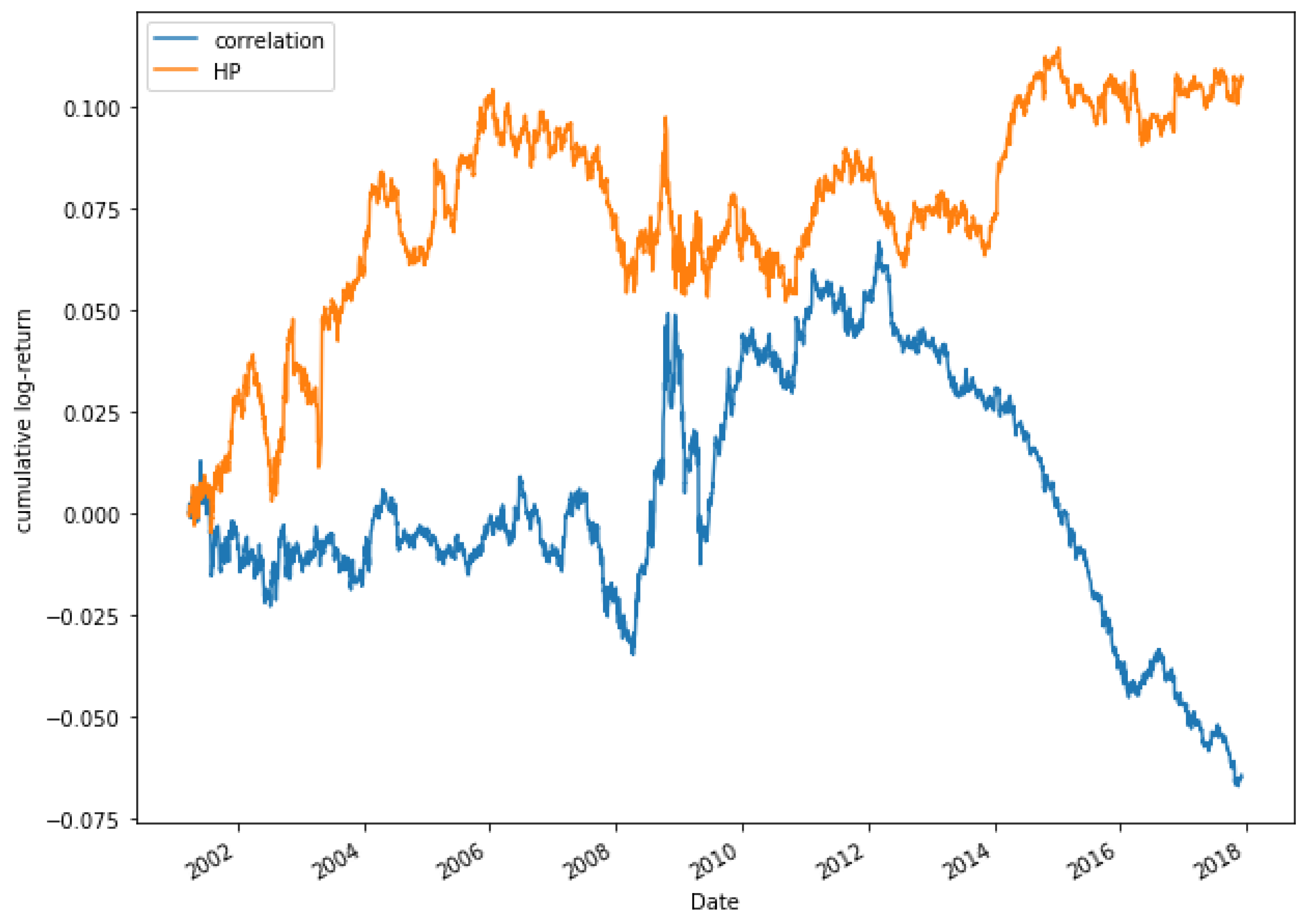
Figure 21 shows the evolution of the two methods for a portfolio of five pairs. It can be observed that during the period the HP model obtains higher returns than the correlation one. In addition, in some moments, the correlation decreases its profitability, while the HP approach increases it. In the case of the portfolio composed of 25 pairs, as shown in Figure 22, the returns are higher through the HP method. It could be pointed out that, from 2012, the correlation model begins to decline, even obtaining negative returns, while the HP approach increases its profitability, reaching its highest peak in 2014.

The empirical results allow concluding that the model presented in this paper is superior to the correlation method in the three scenarios presented, especially in the case of the method called HP2, which is obtained by using 20 days returns (instead of daily returns).

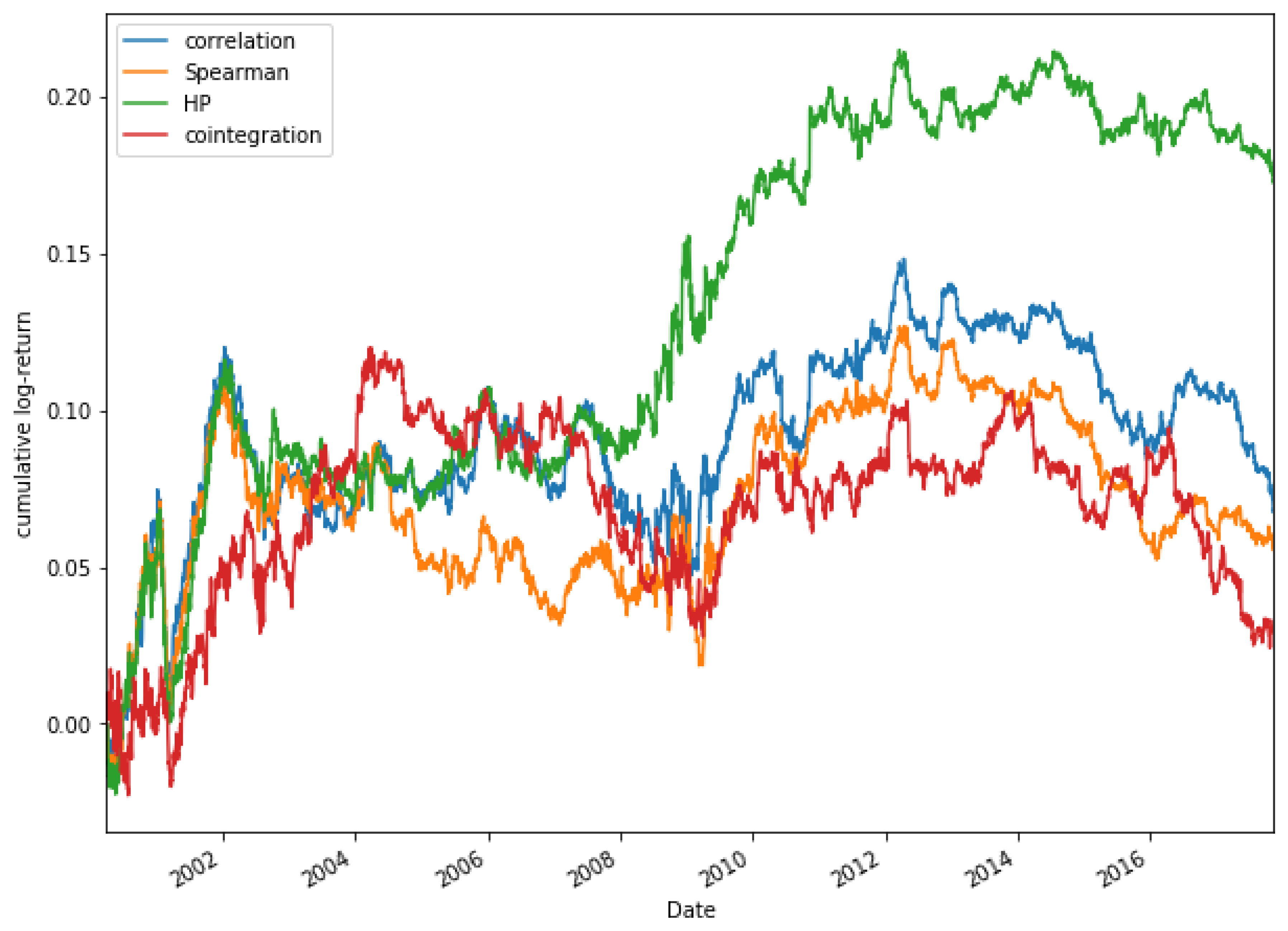
Finally, some other methods to measure correlations are compared in Figure 23, which shows a comparison of the accumulated log-return, for a portfolio composed of 15 pairs, among different methods to measure correlation (Pearson’s correlation coefficient, Spearman’s coefficient and cointegration) and our approach, for the stocks of the Dow Jones and in the period 2000–2018.

In Figure 23, it can be observed that during the period 2000–2004, the accumulated log-returns obtained through the selection of pairs through the Pearson correlation, Spearman correlation and the HP methods are similar. It is not until 2008 that significant differences between the methods used can be found. From that date until the end of the period studied in this paper, it can be observed that the best option is to select the pairs through the HP approach. The accumulated log-returns obtained in this period achieves values between 0.1 and 0.25, obtaining its highest profitability for the period between 2010 and 2014. On the other hand, the results of the rest of the methods are much lower than those obtained by the HP method.

The results obtained allow concluding that the new method (HP) is far superior to the alternative methods used so far to select the pairs through correlation. Therefore it is a novel method that can bring significant benefits to the Pairs Trading strategy.

4. Conclusions

In this paper, a new method (called HP) to measure the dependence between two series was proposed. It was proven that HP is able to detect different kinds of relationships between two series: mainly correlation, but also cointegration and non-linear relationships, even when the relationship is weak or it is given by a copula. The method is especially interesting to study financial series, since it gives more weight to high increments than low increments, contrarily to other correlation measures.

To test the efficiency of this new approach, the HP method was tested through a statistical arbitrage technique for pairs selection and compared with the classical correlation method. Results show that in most cases the HP method performs better.

References

- Markowitz, H. Portfolio Selection. J. Financ. 1952, 7, 77–91. [Google Scholar]
- Roy, A. Safety first and the holding of assets. Econometrica 1952, 20, 431–449. [Google Scholar] [CrossRef]
- Mizuno, T.; Takayasu, H.; Takayasu, M. Correlation networks among currencies. Phys. A Stat. Mech. Its Appl. 2006, 364, 336–342. [Google Scholar] [CrossRef] [Green Version]
- He, L.Y.; Chen, S.P. Multifractal detrended cross-correlation analysis of agricultural futures markets. Chaos Solitons Fractals 2001, 44, 355–361. [Google Scholar] [CrossRef]
- Shiller, R.J.; Beltratti, A.E. Stock prices and bond yields. J. Monet. Econ. 1992, 30, 25–46. [Google Scholar] [CrossRef]
- Gulko, L. Decoupling. J. Portf. Manag. 2002, 28, 59–67. [Google Scholar] [CrossRef]
- Cappiello, L.; Engle, R.F.; Sheppard, K. Asymmetric dynamics in the correlations of global equity and bond returns. J. Financ. Econom. 2006, 4, 537–572. [Google Scholar] [CrossRef]
- Andersson, M.; Krylova, E.; Vähämaa, S. Why does the correlation between stock and bond returns vary over time? Appl. Financ. Econ. 2008, 18, 139–151. [Google Scholar] [CrossRef]
- Lin, W.L.; Engle, R.F.; Ito, T. Do bulls and bears move across borders? International transmission of stock returns and volatility. Rev. Financ. Stud. 1994, 7, 507–538. [Google Scholar] [CrossRef]
- Erb, C.B.; Harvey, C.R.; Viskanta, T.E. Forecasting international correlation. Financ. Anal. J. 1994, 50, 32–45. [Google Scholar] [CrossRef]
- Longinand, F.; Solnik, B. Is the correlation in international equity returns constant: 1960–1990? J. Int. Money Financ. 1995, 14, 3–26. [Google Scholar] [CrossRef]
- Karolyi, G.A.; Stulz, R.M. Why do markets move together? An investigation of U.S.-Japan stock return co-movement. J. Financ. 1996, 51, 951–986. [Google Scholar] [CrossRef]
- De Santis, G.; Gerard, B. International asset pricing and portfolio diversification with time-varying risk. J. Financ. 1997, 52, 1881–1912. [Google Scholar] [CrossRef]
- Ramchand, L.; Susmel, R. Volatility and cross correlation across major stock markets. J. Empir. Financ. 1998, 5, 397–416. [Google Scholar] [CrossRef]
- Solnik, B.; Boucrelle, C.; Le Fur, Y. International market correlation and volatility. Financ. Anal. J. 1996, 52, 17–34. [Google Scholar] [CrossRef]
- Engle, R. Dynamic conditional correlation: A simple class of multivariate generalized autoregressive conditional heteroskedasticity models. J. Bus. Econ. Stat. 2002, 20, 339–350. [Google Scholar] [CrossRef]
- Campbell, R.; Koedijk, K.; Kofman, P. Increased correlation in bear markets. Financ. Anal. J. 2002, 58, 87. [Google Scholar] [CrossRef]
- Jain, P.; Xue, W. Global Investigation of Return Autocorrelation and its Determinants. Pac-Basin Financ. J. 2017, 43, 200–217. [Google Scholar] [CrossRef] [Green Version]
- Gopikrishnan, P.; Plerou, V.; Liu, Y.; Amaral, L.N.; Gabaix, X.; Stanley, H.E. Scaling and correlation in financial time series. Phys. A Stat. Mech. Its Appl. 2000, 287, 362–373. [Google Scholar] [CrossRef]
- Engle, R.F. Autoregressive conditional heteroscedasticity with estimates of the variance of United Kingdom inflation. Econometrica 1982, 50, 987–1007. [Google Scholar] [CrossRef]
- Baillie, R.T.; Bollerslev, T. Intra-day and inter-market volatility in foreign exchange rates. Rev. Econ. Stud. 1991, 58, 565–585. [Google Scholar] [CrossRef]
- Nelson, D.B. Conditional heteroskedasticity in asset returns: A new approach. Econometrica 1991, 59, 347–370. [Google Scholar] [CrossRef]
- Hamilton, J.D.; Susmel, R. Autoregressive conditional heteroskedasticity and changes in regime. J. Econom. 1994, 64, 307–333. [Google Scholar] [CrossRef]
- Cai, J. A Markov model of unconditional variance in ARCH. J. Bus. Econ. Stat. 1994, 12, 309–316. [Google Scholar]
- Ding, Z.; Granger, C.W. Modeling volatility persistence of speculative returns: A new approach. J. Econom. 1996, 73, 185–215. [Google Scholar] [CrossRef]
- Hafner, C.M.; Franses, P.H. A generalized dynamic conditional correlation model: Simulation and application to many assets. Econom. Rev. 2009, 28, 612–631. [Google Scholar] [CrossRef]
- Hurst, H. Long term storage capacity of reservoirs. Trans. Am. Soc. Civ. Eng. 1951, 6, 770–799. [Google Scholar]
- López-García, M.N.; Ramos-Requena, J.P. Different methodologies and uses of the Hurst exponent in econophysics. Estud. Econ. Appl. 2009, 37, 96–108. [Google Scholar] [CrossRef]
- Tatl, H. Detecting persistence of meteorological drought via the Hurst exponent. Meteorol. Appl. 2015, 22, 763–769. [Google Scholar] [CrossRef]
- Singh, A.K.; Bhargawa, A. An early prediction of 25th solar cycle using Hurst exponent. Astrophys. Space Sci. 2017, 362, 199. [Google Scholar] [CrossRef]
- Tong, S.; Zhang, J.; Bao, Y.; Lai, Q.; Lian, X.; Li, N.; Bao, Y. Analyzing vegetation dynamic trend on the Mongolian Plateau based on the Hurst exponent and influencing factors from 1982–2013. J. Geogr. Sci. 2018, 28, 595–610. [Google Scholar] [CrossRef] [Green Version]
- Witton, C.; Sergeyev, S.V.; Turitsyna, E.G.; Furlong, P.L.; Seri, S.; Brookes, M.; Turitsyn, S.K. Rogue bioelectrical waves in the brain: The Hurst exponent as a potential measure for presurgical mapping in epilepsy. J. Neural Eng. 2019, 16, 056019. [Google Scholar] [CrossRef] [PubMed]
- Gao, J.; Hu, J.; Mao, X.; Perc, M. Culturomics meets random fractal theory: Insights into long-range correlations of social and natural phenomena over the past two centuries. J. R. Soc. Interface 2012, 9, 1956–1964. [Google Scholar] [CrossRef] [PubMed] [Green Version]
- Mandelbrot, B.; Wallis, J.R. Robustness of the rescaled range R/S in the measurement of noncyclic long-run statistical dependence. Water Resour. Res. 1969, 5, 967–988. [Google Scholar] [CrossRef]
- Lo, A.W. Long-term memory in stock market prices. Econometrica 1991, 59, 1279–1313. [Google Scholar] [CrossRef]
- Sánchez-Granero, M.A.; Trinida-Segovia, J.E.; García-Pérez, J. Some comments on Hurst exponent and the long memory processes on capital markets. Phys. A Stat. Mech. Its Appl. 2008, 387, 5543–5551. [Google Scholar] [CrossRef]
- Weron, R. Estimating long-range dependence finite sample properties and confidence intervals. Phys. A Stat. Mech. Its Appl. 2002, 312, 285–299. [Google Scholar] [CrossRef] [Green Version]
- Willinger, W.; Taqqu, M.S.; Teverovsky, V. Stock market prices and long-range dependence. Financ. Stoch. 1999, 3, 1–13. [Google Scholar] [CrossRef]
- Sánchez-Granero, M.A.; Trinidad-Segovia, J.E.; García-Pérez, J.; Fernández-Martínez, M. The effect of the underlying distribution in Hurst exponent estimation. PLoS ONE 2015, 10, e0127824. [Google Scholar]
- Geweke, J.; Porter-Hudak, S. The estimation and application of long memory time series models. J. Time Ser. Anal. 1983, 4, 221–238. [Google Scholar] [CrossRef]
- Haslett, J.; Raftery, A.E. Space time modelling with long memory dependence: Assessing Irelands wind power resource. J. R. Stat. Soc. Ser. C (Appl. Stat.) 1989, 38, 1–50. [Google Scholar] [CrossRef]
- Barabasi, A.L.; Vicsek, T. Multifractality of self affine fractals. Phys. Rev. A 1991, 44, 2730–2733. [Google Scholar] [CrossRef] [PubMed]
- Veitch, D.; Abry, P. A wavelet-based joint estimator of the parameters of long-range dependence. IEEE Trans. Inf. Theory 1999, 45, 878–897. [Google Scholar] [CrossRef]
- Alessio, E.; Carbone, A.; Castelli, G.; Frappietro, V. Second-order moving average and scaling of stochastic time series. Eur. Phys. J. B-Condens. Matter Complex Syst. 2002, 27, 197–200. [Google Scholar] [CrossRef]
- Kantelhardt, J.W.; Zschiegner, S.A.; Koscielny-Bunde, E.; Havlin, S.; Bunde, A.; Stanley, H.E. Multifractal detrended fluctuation analysis of nonstationary time series. Phys. A Stat. Mech. Its Appl. 2002, 316, 87–114. [Google Scholar] [CrossRef] [Green Version]
- Bensaida, A. Noisy chaos in intraday financial data: Evidence from the American index. Appl. Math. Comput. 2014, 226, 258–265. [Google Scholar] [CrossRef]
- Das, A.; Das, P. Does composite index of NYSE represents chaos in the long time scale? Appl. Math. Comput. 2006, 174, 483–489. [Google Scholar] [CrossRef]
- Sánchez-Granero, M.A.; Fernández-Martínez, M.; Trinidad-Segovia, J.E. Introducing fractal dimension algorithms to calculate the Hurst exponent of financial time series. Eur. Phys. J. B 2012, 85, 86. [Google Scholar] [CrossRef]
- Fernández-Martínez, M.; Sánchez-Granero, M.A.; Trinidad-Segovia, J.E. Measuring the self-similarity exponent in Levy stable processes of financial time series. Phys. A Stat. Mech. Its Appl. 2013, 392, 5330–5345. [Google Scholar] [CrossRef]
- Barunik, J.; Kristoufek, L. On Hurst exponent estimation under heavy-tailed distributions. Phys. A Stat. Mech. Its Appl. 2010, 389, 3844–3855. [Google Scholar] [CrossRef] [Green Version]
- Embrechts, P.; McNeil, A.J.; Straumann, D. Correlation: Pitfalls and alternatives. Risk 1999, 12, 69–71. [Google Scholar]
- Aas, J. Pair-Copula Constructions for Financial Applications: A Review. Econometrics 2016, 4, 43. [Google Scholar] [CrossRef] [Green Version]
- Joe, H. Families of m-variate distributions with given margins and bivariate dependence parameters. In Distributions with Fixed Marginals and Related Topics; Lecture Notes-Monograph Series, 28; Institute of Mathematical Statistics: Hayward, CA, USA, 1996; pp. 120–141. [Google Scholar]
- Bedford, T.; Cooke, R.M. Probability density decomposition for conditionally dependent random variables modeled by vines. Ann. Math. Artif. Intell. 2001, 32, 245–268. [Google Scholar] [CrossRef]
- Bedford, T.; Cooke, R.M. Vines: A new graphical model for dependent random variables. Ann. Stat. 2002, 30, 1031–1068. [Google Scholar] [CrossRef]
- Aas, K.; Czado, C.; Frigessi, A.; Bakken, H. Pair-copula constructions of multiple dependence. Insur. Math. Econ. 2009, 44, 182–198. [Google Scholar] [CrossRef] [Green Version]
- Czado, C. Analyzing Dependent Data with Vine Copulas; Lecture Notes in Statistics; Springer: Berlin, Germany, 2019. [Google Scholar]
- Pizzutilo, F. A note on the effectiveness of pairs trading for individual investors. Int. J. Econ. Financ. Issues 2013, 3, 763–771. [Google Scholar]
- Vidyamurthy, G. Pairs Trading: Quantitative Methods and Analysis; John Wiley and Sons: Hoboken, NJ, USA, 2004. [Google Scholar]
- Gatev, E.; Goetzmann, W.; Rouwenhorst, K. Pairs trading: Performance of a relative value arbitrage rule. Rev. Financ. Stud. 2006, 19, 797–827. [Google Scholar] [CrossRef] [Green Version]
- Liew, R.Q.; Wu, Y. Pairs trading: A copula approach. J. Deriv. Hedge Funds 2013, 19, 12–30. [Google Scholar] [CrossRef] [Green Version]
- Ramos-Requena, J.P.; Trinidad-Segovia, J.E.; Sánchez-Granero, M.A. Introducing Hurst exponent in pair trading. Phys. A Stat. Mech. Its Appl. 2017, 488, 39–45. [Google Scholar] [CrossRef]
Figure 1.
Histogram of the relationships in correlated series with . The strong correlation is detected by the three methods, though the correlation of the integrated series show some dispersion.
Figure 2.
Histogram of the relationships in correlated series with . Even in weak correlated series, HP is quite high, while the correlation of the integrated series is almost random.
Figure 3.
Histogram of the relationships in cointegrated series with . The cointegration is measured correctly by the three methods when the noise is not high.
Figure 4.
Histogram of the relationships in cointegrated series with . With higher noise, the correlation is quite low, while the HP of the series is still considerably high. Of course, the correlation of the integrated series is the best method to measure this kind of relationship.
Figure 5.
Histogram of the relationships in independent series. In this case, HP and correlation does not show any relationship (because there is no relationship), while the correlation of the integrated series can take almost any value.
Figure 6.
Histogram of the relationships in series with a nonlinear relationship with . While HP is very high, correlation is weak and the correlation of the integrated series is often high, but there is a lot of dispersion.
Figure 7.
Histogram of the relationships in series with a Gaussian copula relationship with . HP is very high, correlation is around as expected and the correlation of the integrated series is often high, but there is a lot of dispersion.
Figure 8.
Histogram of the relationships in series with a Gaussian copula relationship with . Even with a weaker correlation (), HP is high, while the dispersion of the correlation of the integrated series is very high.
Figure 9.
Histogram of the relationships in series with a Student’s t copula relationship with and . HP is very high, correlation is around and the correlation of the integrated series is often high, but there is some dispersion.
Figure 10.
Histogram of the relationships in series with a Student’s t copula relationship with and . Even with a weaker correlation (), HP is high, while the dispersion of the correlation of the integrated series is very high.
Figure 11.
Histogram of the relationships in series with a Student’s t copula relationship with and . With a null correlation, HP is close to and the correlation close to 0, while the dispersion of the correlation of the integrated series is huge.
Figure 12.
Histogram of the relationships in series with a Gumbel copula relationship with . HP is very high, correlation is around and the correlation of the integrated series is often high, but there is a lot of dispersion.
Figure 13.
Histogram of the relationships in series with a Gumbel copula relationship with . Even with a weaker correlation (around ), HP is high, while the dispersion of the correlation of the integrated series is very high.
Figure 14.
Product series of pairs SPY-VHT and GLD-VHT. While the product of the series of the first pair shows a clear persistence (HP ), this is not so for the second pair (HP ).
Figure 15.
Cumulative log-returns of ETFs SPY and VHT. A high degree of co-movement is observed between the two series ().
Figure 16.
Cumulative log-returns of ETFs GLD and VHT. The degree of co-movement is low ().
Figure 17.
Comparative cumulative log-return of a 15-pair portfolio between HP methods and Pearson’s correlation coefficient, of Dow Jones securities in the period 2000–2018.
Figure 18.
Comparative cumulative log-return of a 20-pair portfolio between HP methods and Pearson’s correlation coefficient, of Dow Jones securities in the period 2000–2018.
Figure 19.
Comparative cumulative log-return of a 15-pair portfolio between HP (HP1 version) and Pearson’s correlation coefficient methods, of Dow Jones securities in the period 2000–2018.
Figure 20.
Comparative cumulative log-return of a 20-pair portfolio between HP (HP1 version) and Pearson’s correlation coefficient methods, of Dow Jones securities in the period 2000–2018.
Figure 21.
Comparative cumulative log-return of a 5-pair portfolio between HP (HP2 version) and Pearson’s correlation coefficient methods, of Dow Jones securities in the period 2000–2018.
Figure 22.
Comparative cumulative log-return of a 25-pair portfolio between HP methods (HP2 version) and Pearson’s correlation coefficient, of Dow Jones securities in the period 2000–2018.
Figure 23.
Comparative cumulative log-return of a 15-pair portfolio between Pearson’s correlation coefficient, Spearman’s coefficient, HP and cointegration methods of Dow Jones securities in the period 2000–2018.