Good (and Not So Good) Practices in Computational Methods for Fractional Calculus

Abstract

The solution of fractional-order differential problems requires in the majority of cases the use of some computational approach. In general, the numerical treatment of fractional differential equations is much more difficult than in the integer-order case, and very often non-specialist researchers are unaware of the specific difficulties. As a consequence, numerical methods are often applied in an incorrect way or unreliable methods are devised and proposed in the literature. In this paper we try to identify some common pitfalls in the use of numerical methods in fractional calculus, to explain their nature and to list some good practices that should be followed in order to obtain correct results.

1. Introduction

The increasing interest in applications of fractional calculus, together with the difficulty of finding analytical solutions of fractional differential equations (FDEs), naturally forces researchers to study, devise and apply numerical methods to solve a large range of ordinary and partial differential equations with fractional derivatives.

The investigation of computational methods for fractional-order problems is therefore a very active research area in which, each year, a large number of research papers are published.

The task of finding efficient and reliable numerical methods for handling integrals and/or derivatives of fractional order is a challenge in its own right, with difficulties that differ in character but are no less severe than those associated with finding analytical solutions. The specific nature of these operators involves computational challenges which, if not properly addressed, may lead to unreliable or even wrong results.

Unfortunately, the scientific literature is rich with examples of methods that are inappropriate for fractional-order problems. In most cases these are just methods that were devised originally for standard integer-order operators then applied in a naive way to their fractional-order counterparts; without a proper knowledge of the specific features of fractional-order problems, researchers are often unable to understand why unexpected results are obtained.

The main aims of this paper are to identify a few major guidelines that should be followed when devising reliable computational methods for fractional-order problems, and to highlight the main peculiarities that make the solution of differential equations of fractional order a different—but surely more difficult and stimulating—task from the integer-order case. We do not intend merely to criticize weak or wrong methods, but try to explain why certain approaches are unreliable in fractional calculus and, where possible, point the reader towards more suitable approaches.

This paper is mainly addressed at young researchers or scientists without a particular background in the numerical analysis of fractional-order problems but who need to apply computational methods to solve problems of fractional order. We aim to offer in this way a kind of guide to avoid some of the most common mistakes which, unfortunately, are sometimes made in this field.

The paper is organized in the following way. After recalling in Section 2 some basic definitions and properties, we illustrate in Section 3 the most common ideas underlying the majority of the methods proposed in the literature: very often the basic ideas are not properly recognized and common methods are claimed to be new. In Section 4 we discuss why polynomial approximations can be only partially satisfactory for fractional-order problems and why they are unsuitable for devising high-order methods (as has often been proposed). The major problems related to the nonlocality of fractional operators are addressed in Section 5 and Section 6 discusses some of the most powerful approaches for the efficient treatment of the memory term. Some remarks related to the numerical treatment of fractional partial differential equations are presented in Section 7 and some final comments are given in Section 8.

2. Basic Material and Notations

With the aim of fixing the notation and making available the most common definitions and properties for further reference, we recall here some basic notions concerning fractional calculus.

For $\alpha >0$ and any $t_0\in \mathbb{R}$, in the paper we will adopt the usual definitions for the fractional integral of Riemann–Liouville type

$$J_{t_0}^{\alpha }f(t)=\frac{1}{\Gamma (\alpha )}{\int }_{t_0}^t{(t-\tau )}^{\alpha -1}f(\tau )\mathrm{d}\tau ,t>t_0,$$

(1)

for the fractional derivative of Riemann–Liouville type

$${}^{\mathrm{RL}}{D}_{t_0}^{\alpha }f(t):=D^m{J}_{t_0}^{m-\alpha }f(t)=\frac{1}{\Gamma (m-\alpha )}\frac{{\mathrm{d}}^m}{\mathrm{d}{t}^m}{\int }_{t_0}^t{(t-\tau )}^{m-\alpha -1}f(\tau )\mathrm{d}\tau ,t>t_0$$

(2)

and for the fractional derivative of Caputo type

$${}^{\mathrm{C}}{D}_{t_0}^{\alpha }f(t):=J_{t_0}^{m-\alpha }{D}^{m}f(t)=\frac{1}{\Gamma (m-\alpha )}{\int }_{t_0}^t{(t-\tau )}^{m-\alpha -1}{f}^{(m)}(\tau )\mathrm{d}\tau ,t>t_0,$$

(3)

with $m=⌈\alpha ⌉$ the smallest integer greater than or equal to $\alpha$.

We refer to any of the many existing textbooks on this subject (e.g., [1,2,3,4,5,6]) for an exhaustive treatment of the conditions under which the above operators exist and for their main properties. We just recall here the relationship between ${}^{\mathrm{RL}}{D}_{t_0}^{\alpha }$ and ${}^{\mathrm{C}}{D}_{t_0}^{\alpha }$ expressed as

$${}^{\mathrm{C}}{D}_{t_0}^{\alpha }f(t)={}^{\mathrm{RL}}{D}_{t_0}^{\alpha }\left(f-T_{m-1}[f;t_0]\right)(t),$$

(4)

where $T_{m-1}[f;t_0]$ is the Taylor polynomial of degree $m-1$ for the function f about the point $t_0$,

$$T_{m-1}[f;t_0](t)=\sum _{k=0}^{m-1}\frac{{(t-t_0)}^k}{k!}{f}^{(k)}(t_0).$$

(5)

Moreover, we will almost exclusively consider initial value problems of Cauchy type for FDEs with the Caputo derivative, i.e.,

$$\left\{\begin{array}{c}{}^{\mathrm{C}}{D}_{t_0}^{\alpha }y(t)=f(t,y(t))\hfill \\ y(t_0)=y_0,y^{\prime }(t_0)=y_0^{(1)},\cdots ,y^{(m-1)}(t_0)=y_0^{(m-1)},\hfill \end{array}\right.$$

(6)

for some assigned initial values $y_0,y_0^{(1)},\cdots ,y_0^{(m-1)}$. A few general comments will also be made regarding problems associated with partial differential equations.

3. Novel or Well-Established Methods?

Quite frequently, one sees papers whose promising title claims the presentation of “new methods” or “a family of new methods” for some particular fractional-order operator. Papers of this type immediately capture the attention of readers eager for new and good ideas for numerically solving problems of this type.

But reading the first few pages of such papers can be a source of frustration, since what is claimed to be new is merely an old method applied to a particular (maybe new) problem. Now it is understandable that sometimes an old method is reinvented by a different author, maybe because it can be derived by some different approach or because the author is unaware of the previously published result (perhaps because it was published under an imprecise or misleading title). In fractional calculus, however, a different and quite strange phenomenon has taken hold: well-known and widely used methods are often claimed as “new” just because they are being applied to some specific problem. It seems that some authors are unaware that it is the development of new ideas and new approaches that leads to methods that can be described as new—not the application of known ideas to a particular problem. Even the application of well-established techniques to any of the new operators, obtained by simply replacing the kernel in the integral (1) with some other function, cannot be considered a truly novel method, especially when the extension to the new operator is straightforward.

Most of the papers announcing “new” methods are instead based on ideas and techniques that were proposed and studied decades ago, and sometimes proper references to the original sources are not even given.

In fact, there are a few basic and powerful methods that are suitable and extremely popular for fractional-order problems, and many proposed “new methods” are simply the application of the ideas behind them. It may therefore be useful to illustrate the main and more popular ideas that are most frequently (re)-proposed in fractional calculus, and to outline a short history of their origin and development.

3.1. Polynomial Interpolation and Product-Integration Rules

Solving differential equations by approximating their solution or their vector field by a polynomial interpolant is a very old and common idea. Some of the classical linear multistep methods for ordinary differential equations (ODEs), specifically those of Adams–Bashforth or Adams–Moulton type, are based on this approach.

In 1954 the British mathematician Andrew Young proposed [7,8] the application of polynomial interpolation to solve Volterra integral equations numerically. This approach turns out to be suitable for FDEs since (6) can be reformulated as the Volterra integral equation

$$y(t)=T_{m-1}[f;t_0](t)+\frac{1}{\Gamma (\alpha )}{\int }_{t_0}^t{(t-u)}^{\alpha -1}f(u,y(u))\mathrm{d}u.$$

(7)

The approach proposed by Young is to define a grid $\left\{t_n\right\}$ on the solution interval $[t_0,T]$ (very often, but not necessarily, equispaced, namely $t_n=t_0+hn$, $h=(T-t_0)/N$) and to rewrite (7) in a piecewise way as

$$y(t_n)=T_{m-1}[f;t_0](t_n)+\frac{1}{\Gamma (\alpha )}\sum _{j=0}^{n-1}{\int }_{t_j}^{t_{j+1}}{(t_n-u)}^{\alpha -1}f(u,y(u))\mathrm{d}u,$$

(8)

then to replace, in each interval $[t_j,t_{j+1}]$, the vector field $f(u,y(u))$ by a polynomial that interpolates to f on the grid. This approach is particularly simple if one uses polynomials of degree 0 or 1 because then one can determine the approximation solely on the basis of the data at one of the subinterval’s end points (degree 0; the product rectangle method) or at both end points (degree 1; the product trapezoidal method); thus, in these cases one need not introduce auxiliary points inside the interval or points outside the interval. Neither of these methods can yield a particularly high order of convergence, but as we shall demonstrate in Section 4, the analytic properties of typical solutions to fractional differential equations make it very difficult and cumbersome to achieve high-order accuracy irrespective of the technique used. Consequently, and because these techniques have been thoroughly investigated with respect to their convergence properties [9] and their stability [10] and are hence very well understood, the product rectangle and product trapezoidal methods are highly popular among users of fractional order models.

Higher-order methods have occasionally been proposed [11,12] but—as indicated above and discussed in more detail in Section 4—they tend to require rather uncommon properties of the exact solutions to the given problems and therefore are used only infrequently. We also have to notice that the effects of the lack of regularity on the convergence properties of product-integration rules have been studied since 1985 for Volterra integral equations [13] and since 2004 for the specific case of FDEs [14].

3.2. Approximation of Derivatives: L1 and L2 Schemes

A classical numerical technique for approximating the Caputo differential operator from (3) is the so-called L1 scheme. For $0<\alpha <1$, the definition of the Caputo operator becomes

$${}^{\mathrm{C}}{D}_{t_0}^{\alpha }f(t)=\frac{1}{\Gamma (1-\alpha )}{\int }_{t_0}^t{(t-\tau )}^{-\alpha }{f}^{\prime }(\tau )\mathrm{d}\tau \mathrm{for}t>t_0.$$

The idea ([15], Equation (8.2.6)) is to introduce a completely arbitrary (i.e., not necessarily uniformly spaced) mesh $t_0<t_1<t_2<\dots <t_N$ and to replace the factor $f^{\prime }(\tau )$ in the integrand by the approximation

$$f^{\prime }(\tau )\approx \frac{f(t_{j+1})-f(t_j)}{t_{j+1}-t_j}\mathrm{whenever}\tau \in (t_j,t_{j+1}).$$

This produces the approximation formula

$${}^{\mathrm{C}}{D}_{t_0}^{\alpha }f(t_n)\approx {}^{\mathrm{C}}{D}_{t_0,\mathrm{L}1}^{\alpha }f(t_n)=\frac{1}{\Gamma (2-\alpha )}\sum _{j=0}^{n-1}{w}_{n-j-1,n}(f(t_{n-j})-f(t_{n-j-1}))$$

with

$$w_{\mu ,n}=\frac{{(t_n-t_{\mu })}^{1-\alpha }-{(t_n-t_{\mu +1})}^{1-\alpha }}{t_{n-\mu }-t_{n-\mu -1}}.$$

For smooth functions f (but only under this assumption!) and an equispaced mesh $t_j=t_0+jh$, the convergence order of the L1 method is $\mathcal{O}(h^{2-\alpha })$.

By construction, the L1 method is restricted to the case $0<\alpha <1$. For $\alpha \in (1,2)$, the L2 method ([15], §8.2) provides a useful modification. In its construction, one starts from the representation

$${}^{\mathrm{C}}{D}_{t_0}^{\alpha }f(t)=\frac{1}{\Gamma (2-\alpha )}{\int }_{t_0}^t{t}^{1-\alpha }{f}^{″}(t-\tau )\mathrm{d}\tau ,$$

which is valid for these values of $\alpha$. Using now a uniform grid $t_j=t_0+jh$, one replaces the second derivative of f in the integrand by its central difference approximation,

$$f^{″}(t_n-\tau )\approx \frac{1}{h^2}\left(f(t_n-t_{k+1})-2f(t_n-t_k)+f(t_n-t_{k-1})\right)$$

for $\tau \in [t_k,t_{k+1}]$, which yields

$${}^{\mathrm{C}}{D}_{t_0}^{\alpha }f(t_n)\approx {}^{\mathrm{C}}{D}_{t_0,\mathrm{L}2}^{\alpha }f(t_n)=\frac{h^{-\alpha }}{\Gamma (3-\alpha )}\sum _{k=-1}^n{w}_{k,n}f(t_{n-k}),$$

where now

$$w_{k,n}=\left\{\begin{array}{cc}1\hfill & \mathrm{for}k=-1,\hfill \\ 2^{2-\alpha }-3\hfill & \mathrm{for}k=0,\hfill \\ {(k+2)}^{2-\alpha }-3{(k+1)}^{2-\alpha }+3k^{2-\alpha }-{(k-1)}^{2-\alpha }\hfill & \mathrm{for}1\le k\le n-2,\hfill \\ -2n^{2-\alpha }+3{(n-1)}^{2-\alpha }-{(n-2)}^{2-\alpha }\hfill & \mathrm{for}k=n-1,\hfill \\ n^{2-\alpha }-{(n-1)}^{2-\alpha }\hfill & \mathrm{for}k=n.\hfill \end{array}\right.$$

A disadvantage of this method is that it requires the evaluation for f at the point $t_{n+1}=(n+1)h$ which is located outside the interval $[0,t_n]$.

The central difference used in the definition of the L2 method is symmetric with respect to one of the endpoints of the associated subinterval $[t_k,t_{k+1}]$, not with respect to its mid point. If this is not desired, one may instead use the alternative

$$f^{″}(t_n-\tau )\approx \frac{1}{h^2}\left(f(t_{n-k-2})-f(t_{n-k-1})+f(t_{n-k+1})-f(t_{n-k})\right)$$

on this subinterval. This leads to the L2C method [16]

$${}^{\mathrm{C}}{D}_{t_0}^{\alpha }f(t_n)\approx {}^{\mathrm{C}}{D}_{t_0,\mathrm{L}2C}^{\alpha }f(t_n)=\frac{h^{-\alpha }}{2\Gamma (3-\alpha )}\sum _{k=-1}^{n+1}{w}_{k,n}f(t_{n-k})$$

with

$$w_{k,n}=\left\{\begin{array}{cc}1\hfill & \mathrm{for}k=-1,\hfill \\ 2^{2-\alpha }-2\hfill & \mathrm{for}k=0,\hfill \\ 3^{2-\alpha }-2^{2-\alpha }\hfill & \mathrm{for}k=1,\hfill \\ {(k+2)}^{2-\alpha }-2{(k+1)}^{2-\alpha }+2{(k-1)}^{2-\alpha }-{(k-2)}^{2-\alpha }\hfill & \mathrm{for}2\le k\le n-2,\hfill \\ -n^{2-\alpha }-{(n-3)}^{2-\alpha }+2{(n-2)}^{2-\alpha }\hfill & \mathrm{for}k=n-1,\hfill \\ -n^{2-\alpha }+2{(n-1)}^{2-\alpha }-{(n-2)}^{2-\alpha }\hfill & \mathrm{for}k=n,\hfill \\ n^{2-\alpha }-{(n-1)}^{2-\alpha }\hfill & \mathrm{for}k=n+1.\hfill \end{array}\right.$$

Like the L2 method, the L2C method also requires the evaluation of f outside the interval $[0,t_n]$; one has to compute $f((n+1)h)$ and $f(-h)$. Both the L2 and the L2C method exhibit $\mathcal{O}(h^{3-\alpha })$ convergence behavior for $1<\alpha <2$ if f is sufficiently well behaved; the constants implicitly contained in the $\mathcal{O}$-terms seem to be smaller for the L2 method in the case $1<\alpha <1.5$ and for the L2C method if $1.5<\alpha <2$.

In the limit case $\alpha \to 1$, the L2 method reduces to first-order backward differencing, and the L2C method becomes the centered difference of first order; for $\alpha \to 2$ the L2 method corresponds to the classical second-order central difference.

3.3. Fractional Linear Multistep Methods

Fractional linear multistep methods (FLMMs) are less frequently used since their coefficients are, in general, not known explicitly but it is necessary to devise some algorithm for their (technically often difficult) computation. Nevertheless, since these methods allow us to overcome some of the issues associated with other approaches, it is worth giving a short presentation of their properties.

FLMMs were proposed by Lubich in 1986 [17] and studied in the successive works [18,19,20]. They extend to fractional-order integrals the quadrature rules obtained from standard linear multistep methods (LMMs) for ODEs.

Let us consider a classical k-step LMM of order $p>0$ with first and second characteristic polynomials $\rho (z)={\rho }_0{z}^k+{\rho }_1{z}^{k-1}+\cdots +{\rho }_k$ and $\sigma (z)={\sigma }_0{z}^k+{\sigma }_1{z}^{k-1}+\cdots +{\sigma }_k$, namely

$$\sum _{j=0}^k{\rho }_j{y}_{n-j}=h\sum _{j=0}^k{\sigma }_{j}f(t_{n-j}),\mathrm{where}\delta (\xi )=\frac{\rho (1/\xi )}{\sigma (1/\xi )}\mathrm{is}\mathrm{the}\mathrm{generating}\mathrm{function}.$$

(9)

FLMMs generalizing LMMs (9) for solving FDEs (7) are expressed as

$$y_n=T_{m-1}[f;t_0](t)+h^{\alpha }\sum _{j=0}^{\nu }{w}_{n,j}f(t_j,y_j)+h^{\alpha }\sum _{j=0}^n{\omega }_{n-j}^{(\alpha )}f(t_j,y_j),$$

(10)

where the convolution weights ${\omega }_n^{(\alpha )}$ are obtained from the power series expansion of ${\left(\delta (\xi )\right)}^{-\alpha }$, namely

$$\sum _{n=0}^{\infty }{\omega }_n^{(\alpha )}{\xi }^n=\frac{1}{{\left(\delta (\xi )\right)}^{\alpha }},$$

and the $w_{n,j}$ are some starting weights that are introduced to deal with the lack of regularity of the solution at the origin; they are obtained by solving, at each step n, the algebraic linear systems

$$\sum _{j=0}^{\nu }{w}_{n,j}{j}^{\gamma }=-\sum _{j=0}^n{\omega }_{n-j}{j}^{\gamma }+\frac{\Gamma (\gamma +1)}{\Gamma (1+\gamma +\alpha )}{n}^{\gamma +\alpha },\nu \in {\mathcal{A}}_p,$$

(11)

with ${\mathcal{A}}_p=\left\{\gamma \in \mathbb{R}|\gamma =i+j\alpha ,i,j\in \mathbb{N},\gamma <p-1\right\}$ and $\nu +1$ the cardinality of ${\mathcal{A}}_p$.

The intriguing property of FLMMs is that, unlike product-integration rules, they are able to preserve the same convergence order p of the underlying LMMs if the LMM satisfies certain properties: it is required that $\delta (\xi )$ has no zeros in the closed unit disc $\left|\xi \right|\le 1$ except for $\xi =1$, and $|arg\delta (\xi )|<\pi$ for $\left|\xi \right|<1$. Thus, high-order FLMMs are possible without requiring the imposition of artificial smoothness assumptions as is required for methods based on polynomial interpolation.

But the price to be paid for this advantage may be not negligible: the convolution weights ${\omega }_n^{(\alpha )}$ are not known explicitly and must be computed by some (possibly sophisticated) method (a discussion for the general case is available in [17,18,19,20] while algorithms for FLMMs of trapezoidal type are presented in [21]). Moreover, high-order methods may require the solution of large or very large systems (11) depending on the equation order $\alpha$ and the convergence order p of the method; in some cases these systems are so ill-conditioned as to affect the accuracy of the method, a problem addressed in depth in [22].

One of the simplest methods in this family is obtained from the backward Euler method, whose generating function is $\delta (\xi )=(1-\xi )$. Its convolution weights are hence the coefficients in the asymptotic expansion of ${(1-\xi )}^{-\alpha }$, i.e., they are the coefficients in the binomial series

$${\omega }_j^{(\alpha )}={(-1)}^j\left(\genfrac{}{}{0pt}{}{-\alpha }{j}\right)=\frac{\Gamma (-\alpha +1)}{j!\Gamma (-\alpha -j+1)}$$

and no starting weights are necessary since the convergence order is $p=1$ and hence ${\mathcal{A}}_p$ is the empty set. One recognizes easily that the so-called Grünwald-Letnikov scheme is obtained in this case. Although this scheme was discovered in the nineteenth century in independent works of Grünwald and Letnikov, its interpretation as an FLMM may facilitate its analysis.

4. Classical Approximations Will Not Give High-Order Methods

Solutions of fractional-derivative problems typically exhibit weak singularities. This topic is discussed at length in the survey chapter [23] and it is known since earlier works on Volterra integral equations [24,25]. This singularity is a consequence of the weakly singular behavior of the kernels of integral and fractional derivatives and its importance, from a physical perspective, is related to the natural emergence of completely monotone (CM) relaxation functions in models whose dynamics is governed by these operators [26,27]; CM relaxation behaviors are indeed typical of viscoelastic systems with strongly dissipative energies [28].

In the present section we shall examine the effects of the singular behavior on numerical methods, in the context of initial value problems such as (6).

To grasp quickly the main ideas, we focus on a very simple particular case of (6): the problem

$${}^{\mathrm{C}}{D}_0^{\alpha }y(t)=1\mathrm{for}t\in (0,T],$$

(12)

where $0<\alpha <1$ and, for the moment, we do not prescribe the initial condition at $t=0$. The general solution of (12) is

$$y(t)=\frac{x^{\alpha }}{\Gamma (1+\alpha )}+b,\mathrm{where}b\mathrm{is}\mathrm{an}\mathrm{arbitrary}\mathrm{constant}.$$

(13)

This solution lies in $C[0,T]\cap C^1(0,T]$ but not in $C^1[0,T]$. This implies that standard techniques for integer-derivative problems, which require that $y\in C^1[0,T]$ (or a higher degree of regularity), cannot be used here without some modification. In particular one cannot perform a Taylor series expansion of the solution around $t=0$ because $y^{\prime }(0)$ does not exist.

What about the initial condition? If we prescribe a condition of the form $y(0)=y_0$ we get $b=y_0$ in (13), but the solution is still not in $C^1[0,T]$. One might hope that a Neumann-type condition of the form $y^{\prime }(0)=0$ would control or eliminate the singularity in the solution, but a consideration of (13) shows that it is impossible to enforce such a condition; that is, the problem ${}^{\mathrm{C}}{D}_0^{\alpha }y(t)=1$ on $(0,T]$ with $y^{\prime }(0)=0$ has no solution. This seems surprising until we recall a basic property of the Caputo derivative from ([1], Lemma 3.11): if $m-1<\beta <m$ for some positive integer m and $z\in C^m[0,T]$, then ${lim}_{t\to 0}{}^{\mathrm{C}}{D}_0^{\beta }z(t)=0$. Hence, if in (12) one has $y\in C^1[0,T]$, then taking the limit as $t\to 0$ in (12) we get $0=1$, which is impossible. That is, any solution y of (12) cannot lie in $C^1[0,T]$.

One can present this finding in another way: for the problem ${}^{\mathrm{C}}{D}_0^{\alpha }y(t)=f(t)$ on $(0,T]$ with $f\in C[0,T]$, if the solution $y\in C^1[0,T]$, then one must have $f(0)=0$. This result is a special case of ([1], Theorem 6.26).

Remark 1.

For the problem ${}^{\mathrm{C}}{D}_0^{\alpha }y(t)=f(t)$ on $(0,T]$ with $0<\alpha <1$, if one wants more smoothness of the solution y on the closed interval $[0,T]$, then one must impose further conditions on the data: by ([1], Theorem 6.27), for each positive integer m, one has $y\in C^m[0,T]$ if and only if $0=f(0)=f^{\prime }(0)=\cdots =f^{(m-1)}(0)$.

Conditions such as $f(0)=0$ (and the even stronger conditions listed in Remark 1) impose an artificial restriction on the data f that should be avoided. Thus we continue by looking carefully at the consequence of dealing with a solution of limited smoothness.

Returning to (12) and imposing the initial condition $y(0)=b$, the unique solution of the problem is given by (13), where b is now fixed. Most numerical methods for integer-derivative initial value problems are based on the premise that on any small mesh interval $[t_i,t_{i+1}]$, the unknown solution can be approximated to a high degree of accuracy by a polynomial of suitable degree. But is this true of the function (13)? We now investigate this question.

Consider the interval $[0,h]$, where $h=t_1$. This is the mesh interval where the solution (13) is worst behaved.

Lemma 1.

Let $\alpha \in (0,1)$. Consider the approximation of $t^{\alpha }$ by a linear polynomial $c_0+c_{1}t$ on the interval $[0,h]$. Suppose this approximation is uniformly $\mathcal{O}(h^{\beta })$ accurate on $[0,h]$ for some fixed $\beta >0$. Then one must have $\beta \le \alpha$.

Proof. 

Our hypothesis is that $|t^{\alpha }-(c_0+c_{1}t)|\le C{h}^{\beta }$ for all $t\in [0,h]$ and some constant C that is independent of h and t. Consider the values $t=0,t=h/2$ and $t=h$ in this inequality: we get

$$\left\{\begin{array}{cc}0-(c_0+0)\hfill & =\mathcal{O}(h^{\beta }),\hfill \\ {(h/2)}^{\alpha }-(c_0+c_{1}h/2)\hfill & =\mathcal{O}(h^{\beta }),\hfill \\ h^{\alpha }-(c_0+c_{1}h)\hfill & =\mathcal{O}(h^{\beta }).\hfill \end{array}\right.$$

The first equation gives $c_0=\mathcal{O}(h^{\beta })$. Hence the other equations give ${(h/2)}^{\alpha }-c_{1}h/2=\mathcal{O}(h^{\beta })$ and $h^{\alpha }-c_{1}h=\mathcal{O}(h^{\beta })$. Eliminate $c_1$ by multiplying the first equation by 2 then subtracting from the other equation; this yields $h^{\alpha }-2{(h/2)}^{\alpha }=\mathcal{O}(h^{\beta })$. But this cannot be true unless $\beta \le \alpha$, since the left-hand side is simply a multiple of $h^{\alpha }$ because $\alpha \ne 1$.  □

Lemma 1 says that the approximation of $t^{\alpha }$ on $[0,h]$ by any linear polynomial is at best $\mathcal{O}(h^{\alpha })$. But the order of approximation $\mathcal{O}(h^{\alpha })$ of $t^{\alpha }$ on $[0,h]$ is also achieved by the constant polynomial 0. That is: using a linear polynomial to approximate $t^{\alpha }$ on $[0,h]$ does not give an essentially better result than using a constant polynomial. In a similar way one can show that using polynomials of higher degree does not improve the situation: the order of approximation of $t^{\alpha }$ on $[0,h]$ is still only $\mathcal{O}(h^{\alpha })$. This is a warning that when solving typical fractional-derivative problems, high-degree polynomials may be no better than low-degree polynomials, unlike the classical integer-derivative situation.

One can generalize Lemma 1 to any $\alpha >0$ with $\alpha$ not an integer, obtaining the same result via the same argument. Furthermore, our investigation of the simple problem (12) can be readily generalised to the much more general problem (6); see ([1], Section 6.4).

Implications for the Construction of Difference Schemes

The discussion earlier in Section 4 implies that, to construct higher-order difference schemes for typical solutions of problems such as (12) and (6), one must use non-classical schemes, since the classical schemes are constructed under the assumption that approximations by higher-order polynomials gives greater accuracy. The same idea is developed at length in [29], one of whose results we now present.

Note: although [29] discusses only boundary value problems, an inspection reveals that its arguments and results are also valid (mutatis mutandis) for initial value problems such as (6) when $f=f(t)$, i.e., when the problem (6) is linear.

Let $\alpha >0$ be fixed, with $\alpha$ not an integer. Consider the problem $D^{\alpha }y=f$ on $[0,T]$ with $y(0)=0$. Assume that the mesh on $[0,T]$ is equispaced with diameter h, i.e., $x_i=ih$ for $i=0,1,\cdots ,N$. Suppose that the difference scheme used to solve $D^{\alpha }y=f$ at each point $x_i$ for $i>0$ is ${\sum }_{j=0}^i{a}_{ij}{y}_j^N=f(t_i)$. It is reasonable to assume that $|a_{ij}|=\mathcal{O}(h^{-\alpha })$ for all i and j since we are approximating a derivative of order $\alpha$ (one can check that almost all schemes proposed for this problem have this property).

We have the following variant of ([29], Theorem 3.3).

Theorem 1.

Assume that our scheme achieves order of convergence p for some $p>\alpha$ when $f(t)=C{t}^k$ for all $k\in \{0,1,\cdots ,\lceil p-\alpha -1\rceil \}$. Then for each fixed positive integer i, the coefficients of the scheme must satisfy the following relationship:

$${\displaystyle \underset{h\to 0}{lim}\left(h^{\alpha }\sum _{j=0}^i{j}^{k+\alpha }{a}_{ij}\right)=\frac{i^k\Gamma (\alpha +k+1)}{\Gamma (k+1)}\mathrm{for}k=0,1,\cdots ,\lceil p-\alpha -1\rceil .}$$

(14)

Proof. 

Fix $k\in \{0,1,\cdots ,\lceil p-\alpha -1\rceil \}$. This implies that $k<p-\alpha$. Choose for simplicity

$$f(t)=\frac{\Gamma (k+\alpha +1)}{\Gamma (k+1)}{t}^k.$$

Then the true solution of our initial value problem is $y(t)=t^{k+\alpha }$. Fix a positive integer i. Then

$$\sum _{j=0}^i{a}_{ij}{y}_j^N=f(t_i)=\frac{\Gamma (k+\alpha +1)}{\Gamma (k+1)}{(ih)}^k.$$

Hence, using the hypothesis that our scheme achieves order of convergence p and $|a_{ij}|=\mathcal{O}(h^{-\alpha })$,

$$\begin{array}{cc}\hfill \underset{h\to 0}{lim}\left(h^{\alpha }\sum _{j=0}^i{j}^{k+\alpha }{a}_{ij}\right)& =\underset{h\to 0}{lim}{h}^{-k}\sum _{j=0}^i{a}_{ij}y(t_j)\hfill \\ \hfill & =\underset{h\to 0}{lim}{h}^{-k}\left\{\frac{\Gamma (k+\alpha +1)}{\Gamma (k+1)}{(ih)}^k+\sum _{j=0}^i{a}_{ij}\left[y(x_j)-y_j^N\right]\right\}\hfill \\ \hfill & =\underset{h\to 0}{lim}\left[\frac{\Gamma (k+\alpha +1)}{\Gamma (k+1)}{i}^k+\mathcal{O}(h^{p-\alpha -k})\right]\hfill \\ \hfill & =\frac{\Gamma (k+\alpha +1)}{\Gamma (k+1)}{i}^k,\hfill \end{array}$$

since $k<p-\alpha$.  □

Theorem 1 implies that schemes that fail to satisfy (14) cannot achieve an order of convergence greater than $\mathcal{O}(h^{\alpha })$ at each mesh point. (This is consistent with the approximation theory result of Lemma 1.) For example, in the case $0<\alpha <1$, it follows from Theorem 1 that the well-known L1 scheme is at best $\mathcal{O}(h^{\alpha })$ accurate.

Remark 2.

To avoid the consequences of results such as Theorem 1, one can impose data restrictions such as $f(0)=0$. This is discussed in ([29], Section 5), where theoretical and experimental results show an improvement in the accuracy of standard difference schemes, but only for a restricted class of problems.

5. Failed Approaches to Treat Non-Locality

Non-locality is one of the major features of fractional-order operators. Indeed, fractional integrals and derivatives are often introduced as a mathematical formalism with the primary purpose of encompassing hereditary effects in the modeling of real-life phenomena when theoretical or experimental observations suggest that the effects of external actions do not propagate instantaneously but depend on the history of the system.

On the one hand, non-locality is a very attractive feature that has driven most of the interest and success of the fractional calculus; on the other hand, non-locality introduces severe computational difficulties that researchers try to overcome in different ways.

Unfortunately, some attempts to treat non-locality are unreliable and lead to wrong results. This is the case of the naive implementation of the “finite memory principle” consisting in simply neglecting a large amount of the history solution; since on the basis of this technique it is however possible to devise more sophisticated and accurate approaches, we postpone its discussion to Section 6.

We have also to mention methods based on some kind of fractional Taylor expansion of the solution, such as

$$y(t)=\sum _{k=0}^{\infty }{Y}_k{(t-t_0)}^{k\alpha },$$

where the coefficients $Y_k$ are determined by some suitable numerical technique.

When solving integer-order differential equations, it is possible to use Taylor expansions to approximate the solution at a given point $t_1$ and hence reformulate the same expansion by moving the origin to the new point $t_1$, thus generating a step-by-step method in which the approximation at $t_{n+1}$ is evaluated on the basis of the approximation at $t_n$ (or at additional previous points).

With fractional-order equations, instead, the above expansion holds only with respect to the point $t_0$ (the initial or starting point of the fractional differential operator) and it is not possible to generate a step-by-step method. Expansions of this type are therefore able to provide an accurate approximation only locally, i.e., very close to the starting point $t_0$; consequently, as discussed in [30], methods based on these expansions are usually unsuitable for FDEs.

Another failed approach is based on an attempt to exploit the difference between $y(t_{n+1})$ and $y(t_n)$ in the integral formulation (7): rewrite the solution at $t_{n+1}$ as some increment of the solution at $t_n$, i.e.,

$$y(t_{n+1})=y(t_n)+G_n(t,y(t)),$$

(15a)

then approximate the increment

$$G_n(t,y(t))=\frac{1}{\Gamma (\alpha )}{\int }_{t_0}^{t_{n+1}}{(t_{n+1}-u)}^{\alpha -1}f(u,y(u))\mathrm{d}u-\frac{1}{\Gamma (\alpha )}{\int }_{t_0}^{t_n}{(t_n-u)}^{\alpha -1}f(u,y(u))\mathrm{d}u$$

(15b)

by replacing the vector field $f(t,y(t))$ in both integrals of (15b) by its (first-order) interpolating polynomial at the grid points $t_{n-1}$ and $t_n$. Methods of this kind read as

$$y_{n+1}=y_n+P_n(y_{n-1},y_n),$$

(16)

with $P_n$ a known function obtained by standard interpolation techniques. Approaches of this kind are called two-step Adams–Bashforth methods and attract researchers since they apparently transform the non-local problem into a local one (and thus, a difficult problem into a much easier one); in (15b) $G_n(t,y(t))$ is still a non-local term but these methods are strangely becoming quite popular despite the fact that, as discussed in [31], they are usually unreliable because in most cases they attempt to approximate the (implicitly) non-local contribution $G_n(t,y(t))$ by some purely local term.

Using interpolation at the points $t_{n-1}$ and $t_n$ to approximate $f(t,y(t))$ over the much larger intervals $[t_0,t_n]$ and $[t_0,t_{n+1}]$ is completely inappropriate. It is well known that polynomial interpolation may offer accurate approximations within the interval of the data points, in this case in $[t_{n-1},t_n]$; but outside this interval (where an extrapolation is made instead of an interpolation), the approximation becomes more and more inaccurate as the integration intervals $[t_0,t_n]$ and $[t_0,t_{n+1}]$ in (15b) become larger and larger, i.e., as the integration proceeds and n increases.

The consequence is that completely untrustworthy results must be expected from methods based on this idea.

Note that the fundamental flaw of this approach is not the decomposition (15) but the local (and hence inappropriate) way (16) in which the history is handled. Indeed, it is possible to construct technically correct and efficient algorithms on the basis of (15), for example if one treats the increment term (15b) by a numerical method that is cheaper in computational cost than the method used for the local term [32].

6. Some Approaches for the Efficient, and Reliable, Treatment of the Memory Term

The non-locality of the fractional-order operator means that it is necessary to treat the memory term in an efficient way. This term is commonly identified to be the source of a computational complexity which, especially in problems of large size, requires adequate strategies in order to keep the computational cost at a reasonable level, and indeed this observation has led to many investigations of (more or less successful) approaches to reduce the computational cost. It should be noted however that the high number of arithmetic operations is not the only potential difficulty that the memory term introduces. There is another more fundamental issue, which seems to have attracted much less attention: the history of the process not only needs to be taken into account in the computation but, in order to be properly handled, also needs to be stored in the computer’s memory. While the required amount of memory is usually easily available in algorithms for solving ordinary differential equations, the memory demand may be too high for efficient handling in the case of, e.g., time-fractional partial differential equations where finite element techniques are used to discretize the spatial derivatives.

Most finite-difference methods for FDEs require at each time step the evaluation of some convolution sum of the form

$$y_n={\varphi }_n+\sum _{j=0}^n{c}_j{y}_{n-j}\mathrm{or}{y}_n={\varphi }_n+\sum _{j=0}^n{c}_{j}f(t_{n-j},y_{n-j}),n=1,2,\cdots ,N,$$

(17)

where ${\varphi }_n$ is a term which mainly depends on the initial conditions or other known information.

A naive straightforward evaluation of (17) has a computational cost proportional to $\mathcal{O}\left(N^2\right)$ and, when integration with a small-step size or on a large integration interval is required, the value of N can be extremely large and leads to prohibitive computational costs.

For this reason different approaches for a fast, efficient and reliable treatment of the memory term in non-local problems have been devised. We provide here a short description of some of the most interesting methods of this type. The influence of these approaches on the memory requirements will be addressed as well.

6.1. Nested Mesh Techniques

Several different concepts can be subsumed under the heading of so-called nested meshes. The general idea is based on the observation that the convolution sum in Equation (17) stems from a discretization of a fractional integral or differential operator that uses all the previous grid points as nodes. One can then ask whether it is really neccessary to use all these nodes or whether one could save effort by including only a subset of them by using a second, less fine mesh—i.e., a mesh nested inside the original one.

6.1.1. The Finite Memory Principle

The simplest idea in this class is the finite memory principle ([5], §7.3). It is based on defining a constant $\tau >0$, the so-called memory length, and replacing (for $t>t_0+\tau$) the memory integral term that extends over the interval $[t_0,t]$ by the integral over $[t-\tau ,t]$ with the same integrand function. Technically speaking, this amounts to “forgetting” the entire history of the process that is more than $\tau$ units of time in the past, so the memory has a finite and fixed length $\tau$ instead of the variable length $t-t_0$ that may, in a long running process, be very much longer. From an algorithmic point of view, the finite memory method truncates the convolution sum in Equation (17) to a sum where j runs from $n-\nu$ to n for some fixed $\nu$. This has a number of significant advantages:

• The computational complexity of the nth time step is reduced from $\mathcal{O}(n)$ to $\mathcal{O}(1)$. Therefore, the combined total complexity of the overall method with N time steps is reduced from $\mathcal{O}(N^2)$ to $\mathcal{O}(N)$.
• At no point in time does one need to access the part of the process history that is more than $\nu$ time steps in the past. Therefore, all those previous time steps can be removed from the active memory, and the memory requirement also decreases from $\mathcal{O}(N)$ to $\mathcal{O}(1)$.

Unfortunately, this idea also has severe drawbacks. Specifically, it has been shown in [33] that the convergence order of the underlying discretization technique is lost completely. In other words, one cannot prove that the algorithm converges as the (maximal) step size goes to 0. Therefore, the method is not recommended for practical use.

6.1.2. Logarithmic Memory

To overcome the shortcomings of the finite memory principle, two related but not identical methods, both of which are also based on the nested mesh concept, have been developed in [33,34]. The common idea of both these approaches is the way in which the distant part of the memory is treated. Rather than ignoring it completely as the finite memory principle does, they do sample it, but on a coarser mesh; indeed the fundamental principle is to introduce not just one coarsening level, but to use, say, the step size h on the most recent part of the memory, step size $wh$ (with some parameter $w>1$) on the adjacent region, $w^{2}h$ on the next region, etc. The main difference between the two approaches of [33,34] then lies in the way in which the transition points from one mesh size to the next are chosen.

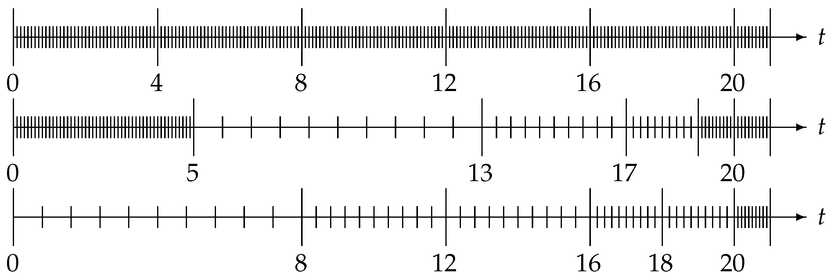
Specifically, as indicated in Figure 1, the method of Ford and Simpson [33] starts at the current time and fills subintervals of prescribed lengths from right to left with appropriately speced mesh points. This will lead to a reduction of the computational cost to $\mathcal{O}(NlogN)$ while retaining the convergence order of the underlying scheme [33]. However, as indicated in Figure 1, it is common that the left end point of the leftmost coarsely subdivided interval does not match the initial point. In this case, one can either fill the remaining subinterval at the left end of the full interval with a fine mesh (which increases the computational cost but also reduces the error) or simply ignore the contribution from this subinterval (which reduces the computational complexity but slightly increases the error; however, since the memory length still grows with the number of steps, this does not imply the complete loss of accuracy observed in the finite memory principle). In either case, grid points from the fine mesh that are not currently used in the nested mesh may become active again in future steps. Therefore, all previous grid points need to be kept in memory, so the required amount of memory space remains at $\mathcal{O}(N)$.

In contrast, the approach of Diethelm and Freed [34] starts to fill the basic interval from left to right, i.e., it begins with the subinterval with the coarsest mesh and then moves to the finer-mesh regions. The final result is also a method with an $\mathcal{O}(NlogN)$ computational cost, and with the same convergence order as the Ford-Simpson method; but its selection strategy for grid points implies that points that are inactive in the current step will never become active again in future steps, and consequently the history data for these inactive points can be eliminated from the main memory. This reduces the memory requirements to only $\mathcal{O}(logN)$.

6.2. A Method Based on the Fast Fourier Transform Algorithm

An effective approach for the fast evaluation of the convolution sums in (17) was proposed in [35,36]. The main idea is to split each of these sums in a way that enables the exploitation of the fast Fourier transform (FFT) algorithm. To provide a concise description, let us introduce the notations

$$T_p(n)=\sum _{j=p}^n{c}_{n-j}{g}_j,S_{p,q}(n)=\sum _{j=p}^q{c}_{n-j}{g}_j,n\ge p,$$

where $g_j=y_j$ or $g_j=f(t_j,y_j)$ according to the formula used in (17). Thus the numerical methods described by (17) can be recast as

$$y_n={\varphi }_n+T_0(n),n=1,2,\cdots ,N.$$

The algorithm described in [35,36] is based on splitting $T_0(n)$ into one or more partial sums of type $S_{p,q}(n)$ and just one final convolution sum $T_p(n)$ of a maximum (fixed) length r. Thus, the computation is simply initialized as

$${\displaystyle T_0(n)=\sum _{j=0}^n{c}_{n-j}{g}_j}n\in \{1,2,\cdots ,r-1\}$$

and the following r values of $T_0(n)$ are split into the two terms

$${\displaystyle T_0(n)=S_{0,r-1}(n)+T_r(n)}n\in \{r,r+1,\cdots ,2r-1\}.$$

Similarly, for the computation of the next $2r$ values, $T_0(n)$ is split according to

$$T_0(n)=\left\{\begin{array}{cc}{S}_{0,2r-1}(n)+T_{2r}(n)\hfill & n\in \{2r,2r+1,\cdots ,3r-1\}\hfill \\ S_{0,2r-1}(n)+S_{2r,3r-1}(n)+T_{3r}(n)\phantom{+S_{2r,3r-1}(n)}\hfill & n\in \{3r,3r+1,\cdots ,4r-1\}\hfill \end{array}\right.$$

and the further $4r$ summations are split according to

$$T_0(n)=\left\{\begin{array}{cc}{\displaystyle S_{0,4r-1}(n)+T_{4r}(n)}\hfill & n\in \{4r,4r+1,\cdots ,5r-1\}\hfill \\ {\displaystyle S_{0,4r-1}(n)+S_{4r,5r-1}(n)+T_{5r}(n)}\hfill & n\in \{5r,5r+1,\cdots ,6r-1\}\hfill \\ {\displaystyle S_{0,4r-1}(n)+S_{4r,6r-1}(n)+T_{7r}(n)}\hfill & n\in \{6r,6r+1,\cdots ,7r-1\}\hfill \\ {\displaystyle S_{0,4r-1}(n)+S_{4r,6r-1}(n)+S_{6r,7r-1}(n)+T_{8r}(n)}\hfill & n\in \{7r,7r+1,\cdots ,8r-1\}\hfill \end{array}\right.$$

and this process is continued until all terms $T_0(n)$, for $n\le N$, are evaluated.

Note that in the above splittings the length $\ell (p,q)=q-p+1$ of each sum $S_{p,q}$ is always some multiple of r with a power of 2 as multiplying factor (i.e., the possible length of $S_{q,p}(n)$ is r, $2r$, $4r$, $8r$ and so on).

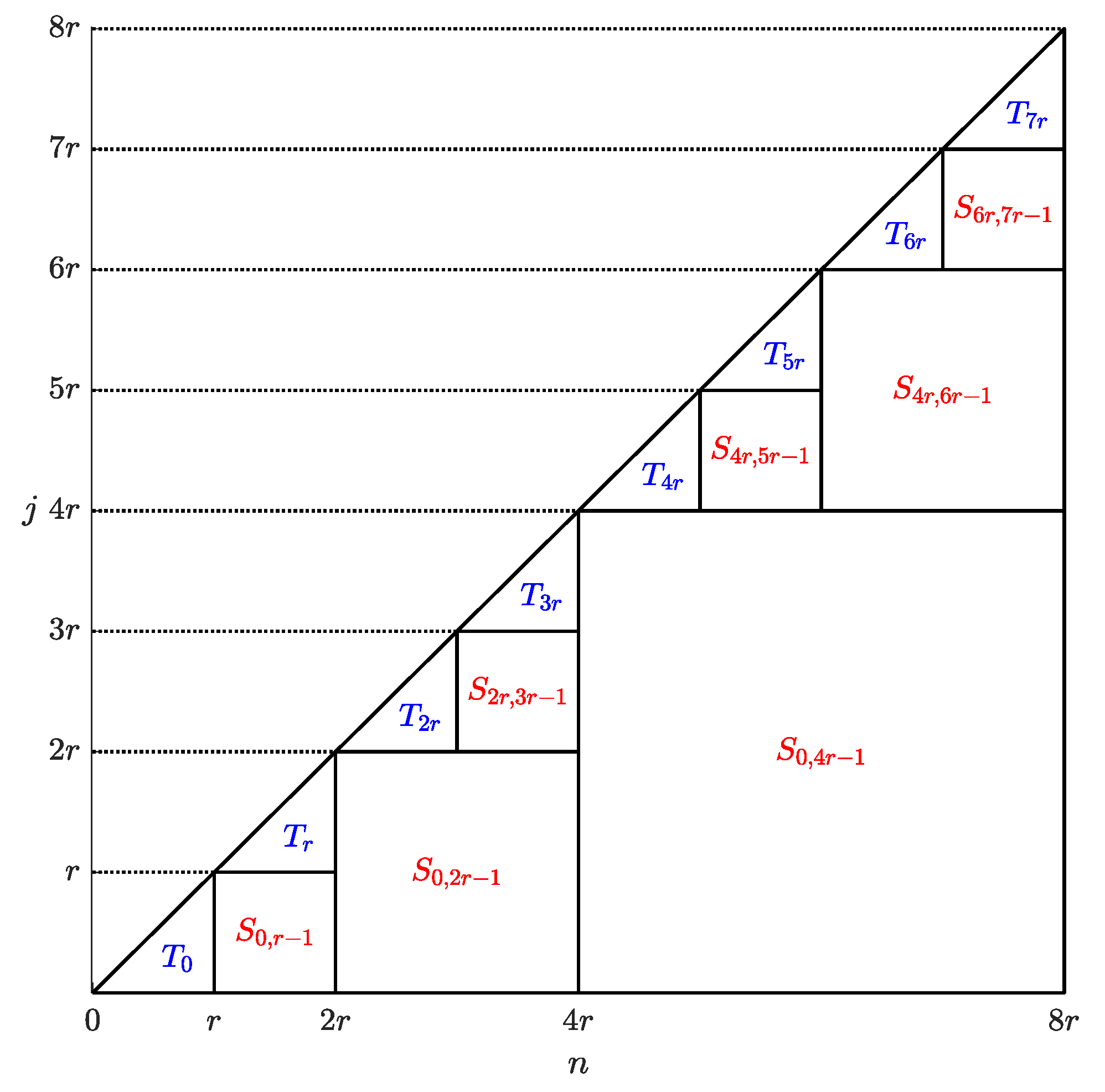
For clarity, the diagram in Figure 2 illustrates the way in which the computation on the main triangle $T_0=\left\{(n,j):0\le j\le n\le N\right\}$ is split into partial sums identified by the (red-labeled) squares $S_{p,q}=\left\{(n,j):q+1\le n\le q+\ell (p,q),p\le j\le q\right\}$ and final blocks denoted by the (blue-labeled) triangles $T_p=\left\{(n,j):p\le j\le n\le p+r-1\right\}$.

Each of the final blocks $T_{\ell r}(n)$, $n=\ell r,\ell r+1,\cdots ,(\ell +1)r-1$, is computed by direct summation requiring $r(r+1)/2$ floating-point operations. The evaluation of the partial sums $S_{q,p}(n)$ can instead be performed by the FFT algorithm (see [37] for a comprehensive description) which requires a number of floating-point operations proportional to $2\ell {log}_{2}2\ell$, with $\ell =\ell (p,q)$ the length of each partial sum $S_{q,p}(n)$, since r is a power of 2.

In the optimal case in which both r and N are powers of 2, each partial sum $S_{p,q}$ that must be computed together with its length, number and computational cost is described in

Table 1. Partial sums, their length, number and computational cost for the evaluation of $T_0(N)$.

Partial Sums	Len.	No.	Cost
$S_{0,\frac{N}{2}-1}$	$\frac{N}{2}$	1	$\mathcal{O}\left(N{log}_{2}N\right)$
$S_{0,\frac{N}{4}-1},S_{\frac{N}{2},\frac{3N}{4}-1}$	$\frac{N}{4}$	2	$\mathcal{O}\left(\frac{N}{2}{log}_2\frac{N}{2}\right)$
$S_{0,\frac{N}{8}-1},S_{\frac{N}{4},\frac{3N}{8}-1},S_{\frac{N}{2},\frac{5N}{8}-1},S_{\frac{3N}{4},\frac{7N}{8}-1}$	$\frac{N}{8}$	4	$\mathcal{O}\left(\frac{N}{4}{log}_2\frac{N}{4}\right)$
$S_{0,\frac{N}{16}-1},S_{\frac{N}{8},\frac{3N}{16}-1},S_{\frac{N}{4},\frac{5N}{16}-1},S_{\frac{3N}{8},\frac{7N}{16}-1},S_{\frac{N}{1},\frac{9N}{16}-1},S_{\frac{5N}{8},\frac{11N}{16}-1},S_{\frac{3N}{4},\frac{13N}{16}-1},S_{\frac{7N}{8},\frac{15N}{16}-1}$	$\frac{N}{16}$	8	$\mathcal{O}\left(\frac{N}{8}{log}_2\frac{N}{8}\right)$
⋮	⋮	⋮	⋮
$S_{0,r-1},S_{2r,3r-1},S_{4r,5r-1},S_{6r,7r-1},S_{8r,9r-1}$,...	r	$s=\frac{N}{2r}$	$\mathcal{O}\left(\frac{N}{s}{log}_2\frac{N}{s}\right)$

.

Furthermore, $N/r$ final blocks $T_{\ell r}$, each of length r, are also computed in $r(r+1)/2$ floating-point operations and hence the total amount of floating point operations is proportional to

$$\begin{array}{cc}\hfill N{log}_{2}N+& 2\left(\frac{N}{2}{log}_2\frac{N}{2}\right)+4\left(\frac{N}{4}{log}_2\frac{N}{4}\right)+\cdots +s\left(\frac{N}{s}{log}_2\frac{N}{s}\right)+\frac{N}{r}\frac{r(r+1)}{2}=\hfill \\ & =\sum _{j=0}^{{log}_{2}s}N{log}_2\frac{N}{2^j}+N\frac{r+1}{2}=\mathcal{O}\left(N{({log}_{2}N)}^2\right),s=\frac{N}{2r},\hfill \end{array}$$

which turns out, for sufficiently large N, to be consistently significantly smaller than the number $\mathcal{O}\left(N^2\right)$ required by the direct summation of $T_0(N)$.

Although the whole procedure may appear complicated and requires some extra effort in coding, it turns out to be quite efficient since it can be applied to different methods of the form (17) and does not affect their accuracy. This preservation of accuracy is because the technique does take into account the entire history of the process in the same way as the straightforward approach mentioned above whose computational cost is $\mathcal{O}(N^2)$. Thus, one does need to keep the entire history data in active memory, but one avoids the requirement of using special meshes. All the Matlab codes for FDEs described in [10,21,38], and freely available on the Mathworks website [39], make use of this algorithm.

6.3. Kernel Compression Schemes

Although the terminology “kernel compression scheme” has been introduced only recently for a few specific works [40,41,42], we use it here to describe a collection of methods that were proposed at various times by various authors and are all based on essentially the same principle: approximation of the solution of a non-local FDE by means of (possibly several) local ODEs. We provide here just the main ideas underlying this approach and we will refer the reader to the literature for a more comprehensive coverage of the subject.

Actually, these are standalone methods (usually classified as nonclassical methods [43]) and not just algorithms improving the efficiency of the treatment of the memory term; for this reason they could have been discussed in Section 3 along with the other methods for FDEs. But since one of their main achievements (and the motivation for their introduction) is to handle memory and computational issues related to the long and persistent memory of fractional-order problems, we consider it appropriate to discuss them in the present section.

For ease of presentation we consider only $0<\alpha <1$ but the extension to any positive $\alpha$ is only a technical matter. The basic idea starts from some integral representation of the kernel of the RL integral (1), e.g.,

$$\frac{t^{\alpha -1}}{\Gamma (\alpha )}=\frac{sin(\alpha \pi )}{\pi }{\int }_0^{\infty }{\mathrm{e}}^{-rt}{r}^{-\alpha }\mathrm{d}r,$$

(18)

which, thanks to standard quadrature rules, can be approximated by exponential sums

$$\frac{t^{\alpha -1}}{\Gamma (\alpha )}=\sum _{k=1}^K{w}_k{\mathrm{e}}^{-r_{k}t}+e_K(t),$$

(19)

where the error $e_K(t)$ and the computational complexity related to the number K of nodes and weights depend on the choice among the many possible quadrature rules. When applying this approximation instead of the exact integral in the integral formulation (7), the solution of the FDE (6) is rewritten as

$$y(t)=y_0+\sum _{k=1}^K{w}_k{\int }_{t_0}^t{\mathrm{e}}^{-r_k(t-u)}f(u,y(u))\mathrm{d}u+E_K(t).$$

(20)

Each of the integrals in (20) is actually the solution of an initial value problem:

$$\left\{\begin{array}{c}{y}^{\left[k\right]}(t)=-r_k{y}^{\left[k\right]}(t)+f(t,y^{\left[k\right]}(t))\hfill \\ y^{\left[k\right]}(t_0)=0,\hfill \end{array}\right.$$

(21)

which can be numerically approximated by standard ODE solvers, yielding approximations $y_n^{\left[k\right]}$ on some grid $\left\{t_n\right\}$. If the quadrature rule is chosen so as to make the error $E_K(t)$ so small that it can be neglected, an approximate solution of the original FDE (6) can be obtained step-by-step as

$$y_n=y_0+\sum _{k=1}^K{\overline{w}}_k{y}_n^{\left[k\right]},$$

where each $y_n^{\left[k\right]}$ depends only on $y_{n-1}^{\left[k\right]}$ or on a few other previous values, according to the selected ODE solver.

In practice, a non-local problem (the FDE) with non-vanishing memory is replaced by K local problems (the ODEs) each demanding a smaller computational effort and the memory storage is restricted to $\mathcal{O}\left(pK\right)$ if a p-step ODE solver is used for each of the ODEs (21).

Obviously, the idea sketched above requires several further technical details to work properly. First, an accurate error analysis is needed to ensure that the overall error is below the target accuracy. This is a very delicate task because it involves the investigation of the interaction between the quadrature rule used to approximate the integral in (20) and the ODE solver applied to the system (21), which can be a highly nontrivial matter. Moreover, some substantial additional problems must be addressed. For instance, A-stable methods should generally be preferred when solving the system (21) since some of the $r_k>0$ can be very large and give rise to stiff problems.

A non-negligible issue is that it is not possible to find a quadrature rule approximating (18) in a uniform manner with respect to all relevant values of t, i.e. with the same accuracy for any $t\ge t_1$ where $t_1$ is the first mesh point to the right of the initial point $t_0$ or for all $t\ge t_0$ (in either case, the singularity at $t_0$ indeed makes the integral quite difficult to be approximated). To overcome this difficulty, several different approaches have been proposed.

In a series of pioneering works [44,45,46], where a complex contour integral

$$\frac{t^{\alpha -1}}{\Gamma (\alpha )}=\frac{1}{2\pi \mathrm{i}}{\int }_{\mathcal{C}}{\mathrm{e}}^{st}{s}^{-\alpha }\mathrm{d}s$$

is chosen to approximate the kernel, the integration interval $[t_0,T]$ is divided into a sequence of subintervals of increasing lengths, and different quadrature rules (on different contours $\mathcal{C}$) are used in each of these intervals. While high accuracy can be obtained, this strategy is quite complicated and requires the use of more expensive complex arithmetic.

In [40,41,42] the integral in (7) is divided into local and history terms

$$y(t)=y_0+\underset{\mathrm{History}\mathrm{term}}{\underbrace{\frac{1}{\Gamma (\alpha )}{\int }_{t_0}^{t-\delta t}{(t-u)}^{\alpha -1}f(u,y(u))\mathrm{d}u}}+\underset{\mathrm{Local}\mathrm{term}}{\underbrace{\frac{1}{\Gamma (\alpha )}{\int }_{t-\delta t}^t{(t-u)}^{\alpha -1}f(u,y(u))\mathrm{d}u}}$$

for a fixed $\delta t>0$. This confines the singularity of the kernel to the local term, which can be approximated by standard methods for weakly singular integral equations (e.g., a product-integration rule) with a reduced computational cost and an insignificant memory requirement. The kernel in the history term no longer contains any singularity and can be safely approximated by (19) which applies now just for $t>\delta t$.

To obtain the highest possible accuracy, Gaussian quadrature rules are usually preferred. A rigorous and technical error analysis is necessary to tune parameters in an optimal way. Several implementations of approaches of this kind have been proposed (e.g., see [47,48,49,50,51]) but owing to their technical nature, a comparison to decide which method is in general the most convenient is difficult; we just refer to the interesting results presented in [52].

7. Some Remarks about Fractional Partial Differential Equations

Even though this paper is essentially devoted to the numerical solution of ordinary differential equations of fractional order and the computational treatment of the associated differential and integral operators, a few comments should be made regarding numerical methods for partial fractional differential equations (PDEs).

Remark 3.

The issues discussed in Section 4 are relevant to partial differential equations also. Indeed, it is shown in [53] that imposing excessive smoothness requirements on the solutions to a partial differential equation (e.g., for the sake of simplifying the error analysis or for obtaining a higher convergence order) has drastic implications regarding the class of admissible problems; in particular, the choice of the forcing function $f(x,t)$ in a linear initial-boundary value problem will then completely determine the initial condition in the problem.

Our second remark regarding partial differential equations deals with a totally different aspect.

Remark 4.

Typical algorithms for time-fractional partial differential equations contain separate discretisation techniques with respect to the time variable and the space variable(s). A current trend is to employ a very high order method for the discretisation of the (non-fractional) differential operator with respect to the space variable. While this might seem an attractive approach at first sight, it has a number of disadvantages. Specifically, while this leads to a smaller discretization error in the space variable, it also increases the algorithm’s overall complexity and makes the understanding of its properties more difficult. This complexity would be acceptable if the overall error could be reduced significantly. But since the overall error comprises not only the error from the space discretisation but also the contribution from the time approximation, it follows that to reduce the overall error, one must force this latter component to be very small also. As indicated above, we cannot expect to achieve a high convergence order in this variable, so the only way to reach this goal is to choose the time step size very small (in comparison with the space mesh size). From Section 6 we conclude that a standard algorithm with a higher-than-linear complexity is likely to lead to prohibitive run times, and even if the time discretisation uses a method with a linear or almost linear complexity, this very small step size requirement will still imply a high overall cost. Therefore, the use of a high-order space discretisation in a time-fractional partial differential equation is usually inadvisable.

8. Concluding Remarks

In this paper we have tried to describe some issues related to the correct use of numerical methods for fractional-order problems. Unlike integer-order ODEs, numerical methods for FDEs are in general not taught in undergraduate courses and, very often, non-specialists are unaware of the peculiarities and major difficulties that arise in the numerical treatment of FDEs and fractional PDEs.

The availability of only a few well-organized textbooks and monographs in this field, together with the presence of many incorrect results in the literature, makes the situation even more difficult.

Some of the ideas collected in this paper were discussed in the lectures of the Training School on “Computational Methods for Fractional-Order Problems”, held in Bari (Italy) during 22–26 July 2019, and promoted by the Cost Action CA15225—Fractional-order systems: analysis, synthesis and their importance for future design.

We believe that the scientific community should make an effort to raise the level of knowledge in this field by promoting specific academic courses at a basic level and/or by organizing training schools.

References

- Diethelm, K. The Analysis of Fractional Differential Equations; Lecture Notes in Mathematics; Springer: Berlin, Germany, 2010; Volume 2004, p. viii+247. [Google Scholar]
- Kilbas, A.A.; Srivastava, H.M.; Trujillo, J.J. Theory and Applications of Fractional Differential Equations; North-Holland Mathematics Studies; Elsevier Science B.V.: Amsterdam, The Netherlands, 2006; Volume 204, p. xvi+523. [Google Scholar]
- Mainardi, F. Fractional Calculus and Waves in Linear Viscoelasticity; Imperial College Press: London, UK, 2010; p. xx+347. [Google Scholar]
- Miller, K.S.; Ross, B. An Introduction to the Fractional Calculus and Fractional Differential Equations; A Wiley-Interscience Publication; John Wiley & Sons, Inc.: New York, NY, USA, 1993; p. xvi+366. [Google Scholar]
- Podlubny, I. Fractional Differential Equations; Mathematics in Science and Engineering; Academic Press Inc.: San Diego, CA, USA, 1999; Volume 198, p. xxiv+340. [Google Scholar]
- Samko, S.G.; Kilbas, A.A.; Marichev, O.I. Fractional Integrals and Derivatives; Gordon and Breach Science Publishers: Yverdon, Switzerland, 1993; p. xxxvi+976. [Google Scholar]
- Young, A. Approximate product-integration. Proc. R. Soc. Lond. Ser. A 1954, 224, 552–561. [Google Scholar]
- Young, A. The application of approximate product integration to the numerical solution of integral equations. Proc. R. Soc. Lond. Ser. A 1954, 224, 561–573. [Google Scholar]
- Diethelm, K.; Ford, N.J.; Freed, A.D. A predictor-corrector approach for the numerical solution of fractional differential equations. Nonlinear Dyn. 2002, 29, 3–22. [Google Scholar] [CrossRef]
- Garrappa, R. On linear stability of predictor-corrector algorithms for fractional differential equations. Int. J. Comput. Math. 2010, 87, 2281–2290. [Google Scholar] [CrossRef]
- Yan, Y.; Pal, K.; Ford, N.J. Higher order numerical methods for solving fractional differential equations. BIT Numer. Math. 2014, 54, 555–584. [Google Scholar] [CrossRef] [Green Version]
- Li, Z.; Liang, Z.; Yan, Y. High-order numerical methods for solving time fractional partial differential equations. J. Sci. Comput. 2017, 71, 785–803. [Google Scholar] [CrossRef] [Green Version]
- Dixon, J. On the order of the error in discretization methods for weakly singular second kind Volterra integral equations with nonsmooth solutions. BIT 1985, 25, 624–634. [Google Scholar] [CrossRef]
- Diethelm, K.; Ford, N.J.; Freed, A.D. Detailed error analysis for a fractional Adams method. Numer. Algorithms 2004, 36, 31–52. [Google Scholar] [CrossRef] [Green Version]
- Oldham, K.B.; Spanier, J. Theory and applications of differentiation and integration to arbitrary order. In The Fractional Calculus; Academic Press: New York, NY, USA; London, UK, 1974; p. xiii+234. [Google Scholar]
- Lynch, V.E.; Carreras, B.A.; del Castillo-Negrete, D.; Ferreira-Mejias, K.M.; Hicks, H.R. Numerical methods for the solution of partial differential equations of fractional order. J. Comput. Phys. 2003, 192, 406–421. [Google Scholar] [CrossRef]
- Lubich, C. Discretized fractional calculus. SIAM J. Math. Anal. 1986, 17, 704–719. [Google Scholar] [CrossRef]
- Lubich, C. Convolution quadrature and discretized operational calculus. I. Numer. Math. 1988, 52, 129–145. [Google Scholar] [CrossRef]
- Lubich, C. Convolution quadrature and discretized operational calculus. II. Numer. Math. 1988, 52, 413–425. [Google Scholar] [CrossRef]
- Lubich, C. Convolution quadrature revisited. BIT 2004, 44, 503–514. [Google Scholar] [CrossRef]
- Garrappa, R. Trapezoidal methods for fractional differential equations: theoretical and computational aspects. Math. Comput. Simul. 2015, 110, 96–112. [Google Scholar] [CrossRef] [Green Version]
- Diethelm, K.; Ford, J.M.; Ford, N.J.; Weilbeer, M. Pitfalls in fast numerical solvers for fractional differential equations. J. Comput. Appl. Math. 2006, 186, 482–503. [Google Scholar] [CrossRef] [Green Version]
- Stynes, M. Singularities. In Handbook of Fractional Calculus With Applications; De Gruyter: Berlin, Germany, 2019; Volume 3, pp. 287–305. [Google Scholar]
- Miller, R.K.; Feldstein, A. Smoothness of solutions of Volterra integral equations with weakly singular kernels. SIAM J. Math. Anal. 1971, 2, 242–258. [Google Scholar] [CrossRef] [Green Version]
- Lubich, C. Runge-Kutta theory for Volterra and Abel integral equations of the second kind. Math. Comput. 1983, 41, 87–102. [Google Scholar] [CrossRef]
- Hanyga, A. A comment on a controversial issue: A generalized fractional derivative cannot have a regular kernel. Fract. Calc. Appl. Anal. 2020, 23, 211–223. [Google Scholar] [CrossRef] [Green Version]
- Giusti, A. General fractional calculus and Prabhakar’s theory. Commun. Nonlinear Sci. Numer. Simul. 2019, 83, 105114. [Google Scholar] [CrossRef] [Green Version]
- Hanyga, A. Physically acceptable viscoelastic models. In Trends in Applications of Mathematics to Mechanics; Hutter, K., Wang, Y., Eds.; Shaker Verlag: Aachen, Germany, 2005; pp. 125–136. [Google Scholar]
- Stynes, M.; O’Riordan, E.; Gracia, J.L. Necessary conditions for convergence of difference schemes for fractional-derivative two-point boundary value problems. BIT 2016, 56, 1455–1477. [Google Scholar] [CrossRef]
- Sarv Ahrabi, S.; Momenzadeh, A. On failed methods of fractional differential equations: the case of multi-step generalized differential transform method. Mediterr. J. Math. 2018, 15, 149. [Google Scholar] [CrossRef] [Green Version]
- Garrappa, R. Neglecting nonlocality leads to unreliable numerical methods for fractional differential equations. Commun. Nonlinear Sci. Numer. Simul. 2019, 70, 302–306. [Google Scholar] [CrossRef] [Green Version]
- Deng, W.H. Short memory principle and a predictor-corrector approach for fractional differential equations. J. Comput. Appl. Math. 2007, 206, 174–188. [Google Scholar] [CrossRef] [Green Version]
- Ford, N.J.; Simpson, A.C. The numerical solution of fractional differential equations: Speed versus accuracy. Numer. Algorithms 2001, 26, 333–346. [Google Scholar] [CrossRef]
- Diethelm, K.; Freed, A.D. An Efficient Algorithm for the Evaluation of Convolution Integrals. Comput. Math. Appl. 2006, 51, 51–72. [Google Scholar] [CrossRef] [Green Version]
- Hairer, E.; Lubich, C.; Schlichte, M. Fast numerical solution of nonlinear Volterra convolution equations. SIAM J. Sci. Statist. Comput. 1985, 6, 532–541. [Google Scholar] [CrossRef]
- Hairer, E.; Lubich, C.; Schlichte, M. Fast numerical solution of weakly singular Volterra integral equations. J. Comput. Appl. Math. 1988, 23, 87–98. [Google Scholar] [CrossRef]
- Henrici, P. Fast Fourier methods in computational complex analysis. SIAM Rev. 1979, 21, 481–527. [Google Scholar] [CrossRef]
- Garrappa, R. Numerical Solution of Fractional Differential Equations: A Survey and a Software Tutorial. Mathematics 2018, 6, 16. [Google Scholar] [CrossRef] [Green Version]
- Garrappa, R. Mathworks Author’s Profile. Available online: https://www.mathworks.com/matlabcentral/profile/authors/2361481-roberto-garrappa (accessed on 26 January 2020).
- Baffet, D. A Gauss-Jacobi kernel compression scheme for fractional differential equations. J. Sci. Comput. 2019, 79, 227–248. [Google Scholar] [CrossRef] [Green Version]
- Baffet, D.; Hesthaven, J.S. A kernel compression scheme for fractional differential equations. SIAM J. Numer. Anal. 2017, 55, 496–520. [Google Scholar] [CrossRef] [Green Version]
- Baffet, D.; Hesthaven, J.S. High-order accurate adaptive kernel compression time-stepping schemes for fractional differential equations. J. Sci. Comput. 2017, 72, 1169–1195. [Google Scholar] [CrossRef]
- Diethelm, K. An investigation of some nonclassical methods for the numerical approximation of Caputo-type fractional derivatives. Numer. Algorithms 2008, 47, 361–390. [Google Scholar] [CrossRef]
- López-Fernández, M.; Lubich, C.; Schädle, A. Adaptive, fast, and oblivious convolution in evolution equations with memory. SIAM J. Sci. Comput. 2008, 30, 1015–1037. [Google Scholar] [CrossRef] [Green Version]
- Lubich, C.; Schädle, A. Fast convolution for nonreflecting boundary conditions. SIAM J. Sci. Comput. 2002, 24, 161–182. [Google Scholar] [CrossRef]
- Schädle, A.; López-Fernández, M.; Lubich, C. Fast and oblivious convolution quadrature. SIAM J. Sci. Comput. 2006, 28, 421–438. [Google Scholar] [CrossRef] [Green Version]
- Banjai, L.; López-Fernández, M. Efficient high order algorithms for fractional integrals and fractional differential equations. Numer. Math. 2019, 141, 289–317. [Google Scholar] [CrossRef] [Green Version]
- Fischer, M. Fast and parallel Runge-Kutta approximation of fractional evolution equations. SIAM J. Sci. Comput. 2019, 41, A927–A947. [Google Scholar] [CrossRef] [Green Version]
- Jiang, S.; Zhang, J.; Zhang, Q.; Zhang, Z. Fast evaluation of the Caputo fractional derivative and its applications to fractional diffusion equations. Commun. Comput. Phys. 2017, 21, 650–678. [Google Scholar] [CrossRef]
- Li, J.R. A fast time stepping method for evaluating fractional integrals. SIAM J. Sci. Comput. 2010, 31, 4696–4714. [Google Scholar] [CrossRef] [Green Version]
- Zeng, F.; Turner, I.; Burrage, K. A stable fast time-stepping method for fractional integral and derivative operators. J. Sci. Comput. 2018, 77, 283–307. [Google Scholar] [CrossRef] [Green Version]
- Guo, L.; Zeng, F.; Turner, I.; Burrage, K.; Karniadakis, G.E.M. Efficient multistep methods for tempered fractional calculus: Algorithms and simulations. SIAM J. Sci. Comput. 2019, 41, 2510–2535. [Google Scholar] [CrossRef] [Green Version]
- Stynes, M. Too much regularity may force too much uniqueness. Fract. Calc. Appl. Anal. 2016, 19, 1554–1562. [Google Scholar] [CrossRef] [Green Version]
Figure 1.
Full mesh (top) and nested meshes proposed in [33] (center) and in [34] (bottom). The meshes are shown for the time instant and the basic step size .
Figure 2.
Splitting of the computation of into partial sums (red-labeled squares) and final blocks (blue-labeled triangles).