Regarding New Wave Patterns of the Newly Extended Nonlinear (2+1)-Dimensional Boussinesq Equation with Fourth Order

Abstract

This paper applies the sine-Gordon expansion method to the extended nonlinear (2+1)-dimensional Boussinesq equation. Many new dark, complex and mixed dark-bright soliton solutions of the governing model are derived. Moreover, for better understanding of the results, 2D, 3D and contour graphs under the strain conditions and the suitable values of parameters are also plotted.

1. Introduction

This century, soliton theory has been one of the most important theories of nonlinear sciences. Mathematically, one of such fields where this theory has been considered has the aim of explaining the propagation of water waves. Such wave propagation has been observed in quantum mechanics, electricity, optical soliton, optical fibers, viscoelasticity, mathematics, physics, chemistry and in many other areas. A lot of researchers from all over the world have developed various methods to investigate new properties of this propagation: the variational iteration method [1], the modified simply equation method [2], the simplified Hirota’s method [3], the extended tanh method [4,5], the tanh method [6], the inverse scattering transform method [7], Hirota’s bilinear method [8], the sine-Gordon expansion method [9], the $\left(\frac{G^{\prime }}{G}\right)$ expansion method [10], the tanh and extended tanh methods [11], the new Jacobi elliptic function expansion method [12], the extended and generalized tanh-function method [13,14,15], the hyperbolic ansatz method [16], the rational sinh-cosh method and so on [17,18,19,20,21,22,23,24,25,26,27,28,29]. One of these water wave propagations belongs to the Boussinesq who proposed a model in 1871 given as

$$u_{tt}-u_{xx}+\beta {\left(u^2\right)}_{xx}+\gamma u_{xxxx}=0,$$

where $\beta$ and $\gamma$ are real constants with non-zero figures. The Boussinesq equation can be further divided into two cases: the good Boussinesq (BSQ) equation with $\gamma >0$, and the bad Boussinesq equation with $\gamma <0$. Hirota was among the first one who solved the bad Boussinesq equation ($\gamma <0$) for the multi-soliton solution [30]. After then, several other types of solutions of this equation were obtained in [31] by using the Wronskian formulation. As for the good Boussinesq equation with $\gamma >0$, the multi-soliton solution was derived in [32] by using the Hirota method. In that work, the bilinear form of the good BSQ equation was obtained and the multi-soliton solution was subsequently derived from that transformed bilinear equation. A rigourous proof was also provided in [32]. The Wronskian formulation of the good Boussinesq equation can be derived and found in [33]. Several kinds of solutions, including solitons, negations, positions and complexitons, were found by using this Wronskian formulation. The above-mentioned works employed the Hirota bilinear form of the Boussinesq equation to derive the analytical solutions. A systematic method for deriving such a bilinear form is the homogeneous balance method. In fact, a modified version of this method was introduced in [34] to extend the Hirota bilinear form of the Boussinesq equation which had been derived in [30].

This model describes the propagation of shallow water waves within the small amplitudes as they propagate at a uniform speed in a water canal of constant depth. Moreover, it arises in several other fluid dynamical theories. Investigating deeper into properties of this model, some powerful methods [35,36] have been applied successfully. One model based on this equation, namely, the extended nonlinear (2+1)-dimensional Boussinesq equation [37,38] defined by

$$u_{tt}+\alpha u_{yt}-\alpha u_{yy}+{\alpha }_1ϵu_{xy}+{\alpha }_2ϵ{\left(u^2\right)}_{xx}+{\alpha }_3{ϵ}^2{u}_{xxxx}=0,{ϵ}^2=\pm 1,$$

(1)

was newly presented to the literature. In Equation (1), $\alpha ,{\alpha }_1,{\alpha }_2$ and ${\alpha }_3$ are real constants and non-zero. Equation (1) has been derived from the Boussinesq model which is used to explain water waves arising in fluid dynamics as special cases of Whitham theory [39,40].

This paper is distributed in different sections. In Section 2, we present the general properties of sine-Gordon expansion method (SGEM) in a detailed manner. In Section 3, we apply SGEM to the Equation (1) to extract many new dark, complex and mixed dark-bright soliton solutions. Moreover, strain conditions are also derived for validity of results. In the last section, we underline the novelty of these results via a conclusion section.

2. General Facts of SGEM

In this section we shall consider the following sine-Gordon equation [41]:

$$u_{xx}(x,t)-u_{tt}(x,t)=m^{2}sin\left(u(x,t)\right),$$

(2)

in which m is a real non-zero constant. When we apply the traveling wave transformation as $u(x,t)=U\left(\xi \right),$$\xi =\mu (x-ct)$ into Equation (2), it may be rewritten as the following nonlinear ordinary differential equation (NODE):

$$U^{{}^{″}}=\frac{m^2}{{\mu }^2(1-c^2)}sin\left(U\right),$$

(3)

where $U=U\left(\xi \right)$, $U^{{}^{″}}=\frac{d^{2}U}{d{\xi }^2}$ and c, $\mu$, are also non-zero real constants. Integrating Equation (3) by multiplying $U^{\prime }$ both sides for calculating, we obtain

$${\left({\left(\frac{U}{2}\right)}^{{}^{\prime }}\right)}^2=\frac{m^2}{{\mu }^2(1-c^2)}{sin}^2\left(\frac{U}{2}\right)+k,$$

(4)

where k is an integral constant. For simplicity, we consider $k=0,w=\frac{U}{2},$ and $a^2=\frac{m^2}{{\mu }^2(1-c^2)},$ Equation (4) reads as

$$w^{{}^{\prime }}=asin\left(w\right),$$

(5)

where $w=w\left(\xi \right)$. By taking $a=1$ in Equation (5), we obtain the following two interesting and important relationships

$$sin\left(w\right)=sin\left[w\left(\xi \right)\right]=\frac{2p{e}^{\xi }}{p^2{e}^{2\xi }+1}\downarrow p_{=1}=\mathrm{sech}\left(\xi \right),$$

(6)

$$cos\left(w\right)=cos\left[w\left(\xi \right)\right]=\frac{2p{e}^{\xi }}{p^2{e}^{2\xi }+1}\downarrow p_{=1}=\tanh \left(\xi \right).$$

(7)

We shall consider in a general case the following nonlinear partial differential equation defined by

$$P(u,u_x,u_{xt},u^2,\cdots )=0.$$

(8)

In Equation (8), by applying the traveling wave transform as $u=u(x,t)=U\left(\xi \right),\xi =\mu (x-ct)$, we obtain the following NODE

$$N(U,U^{\prime },U^{\prime \prime },U^2,\cdots )=0.$$

(9)

where $U=U\left(\xi \right)$, $U^{{}^{\prime }}=\frac{dU}{d\xi }$. In this NODE, supposing the trial solution function may be considered as

$$U\left(\xi \right)=\sum _{i=1}^n{\tanh }^{i-1}\left(\xi \right)[B_i\mathrm{sech}\left(\xi \right)+A_1\tanh \left(\xi \right)]+A_0.$$

(10)

Equation (10) may be rewritten with the help of Equations (6) and (7) as following

$$U\left(w\right)=\sum _{i=1}^n{cos}^{i-1}\left(w\right)[B_{i}sin\left(w\right)+A_{1}cos\left(w\right)]+A_0.$$

(11)

in which the value of n will be determined later via balance principle. After putting the necessary derivations of Equation (11) into Equation (9), we obtain an equation of ${sin}^i\left(w\right){cos}^j\left(w\right)$. Taking all these terms to zero yields a system of equations. Solving this system by using some computational programs, gives the values of $A_i,B_i,\mu$ and c. Via these values of parameters $A_i,B_i,\mu$ and c in Equation (10), we obtain the new traveling wave solutions to Equation (8).

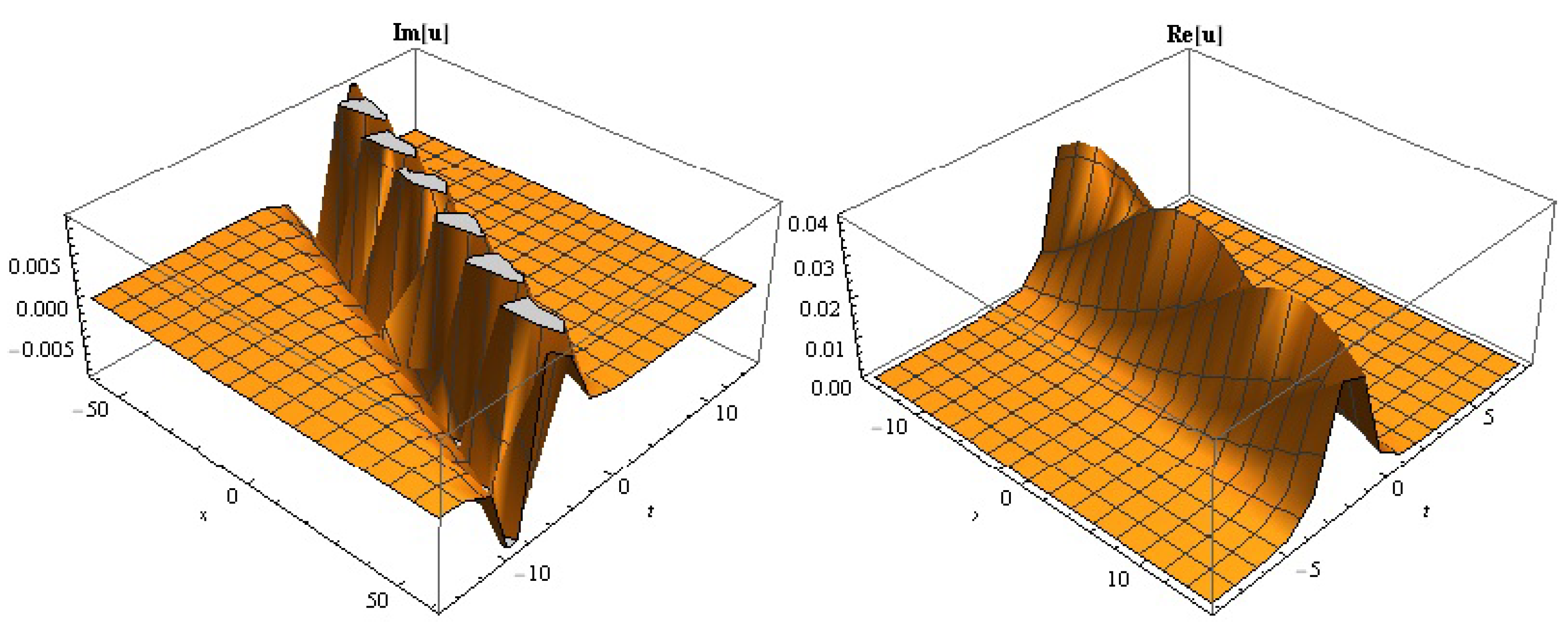
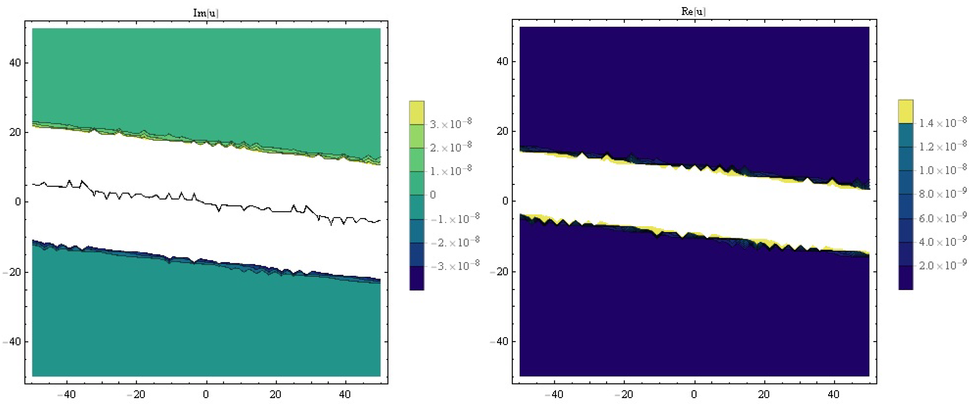
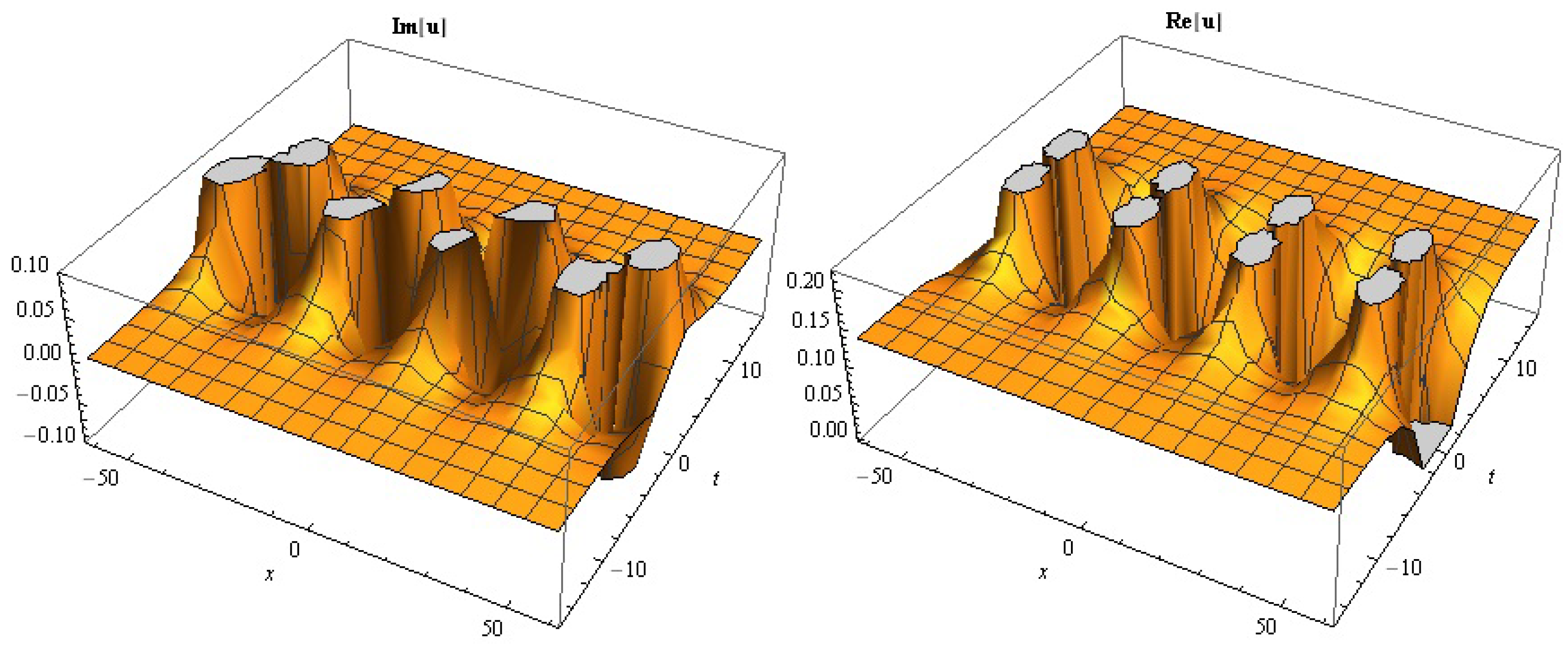
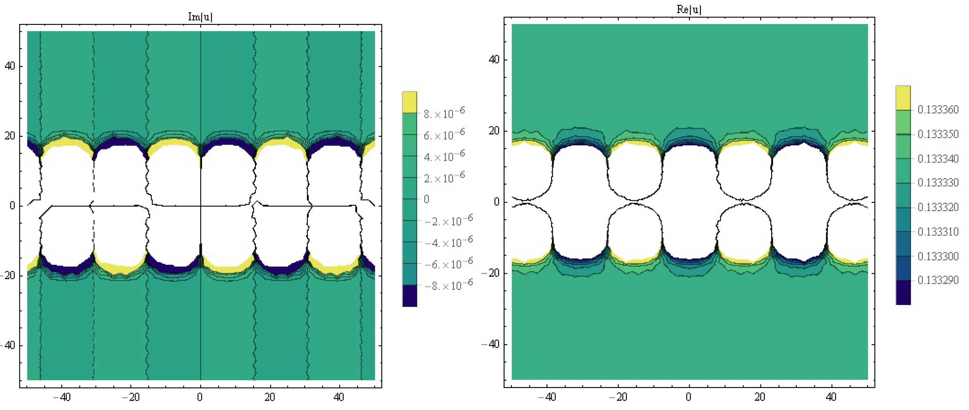
3. Application of SGEM

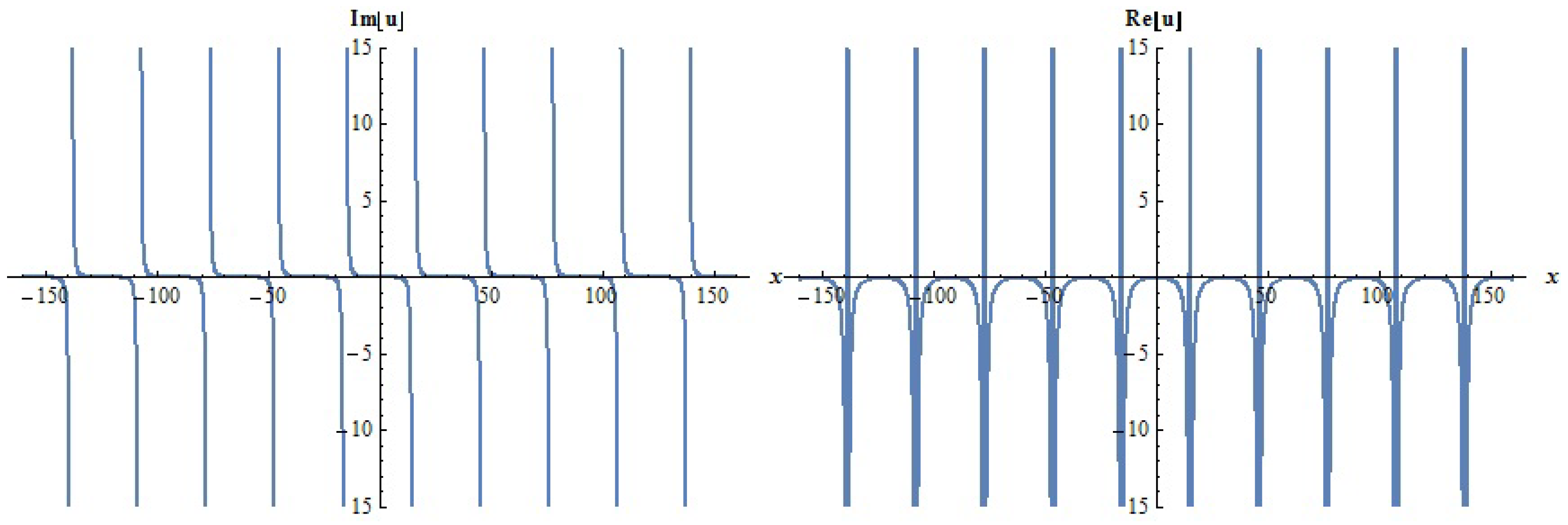
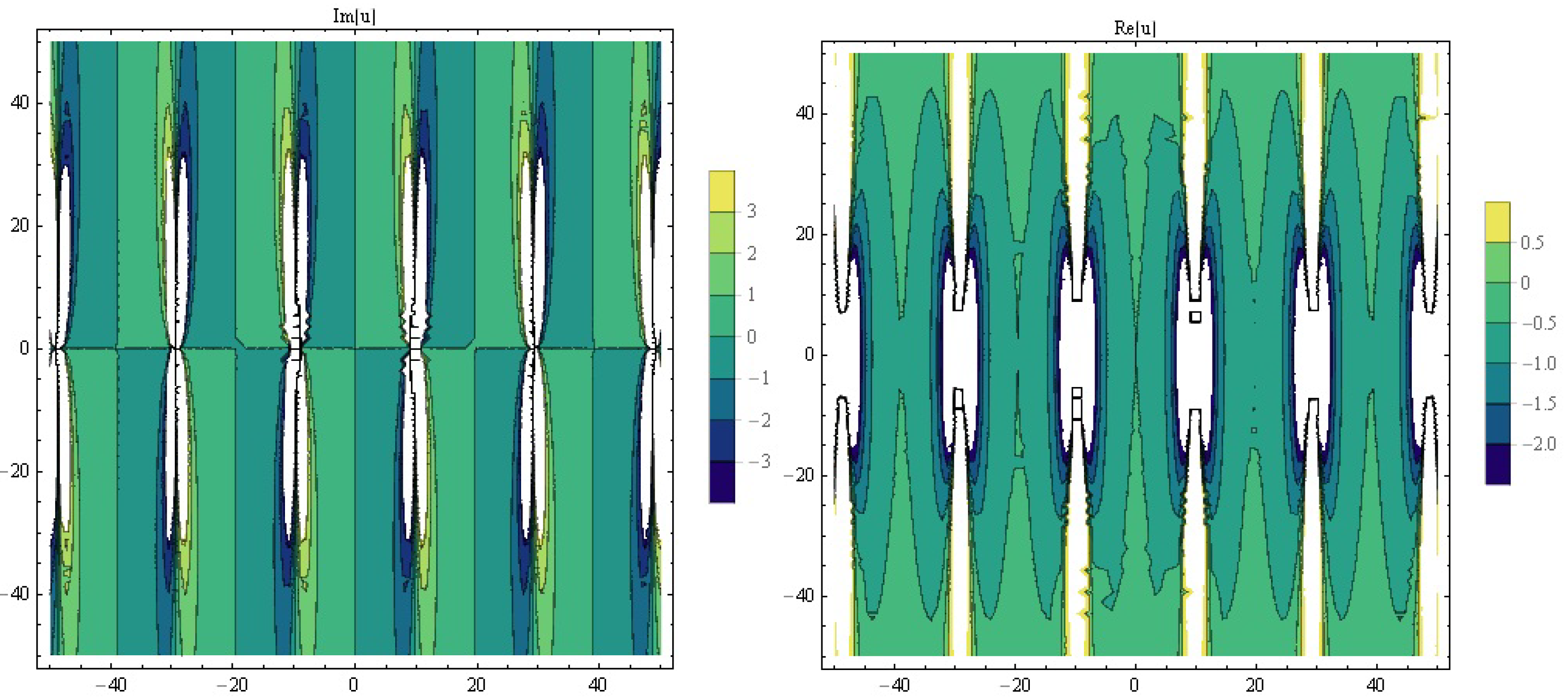
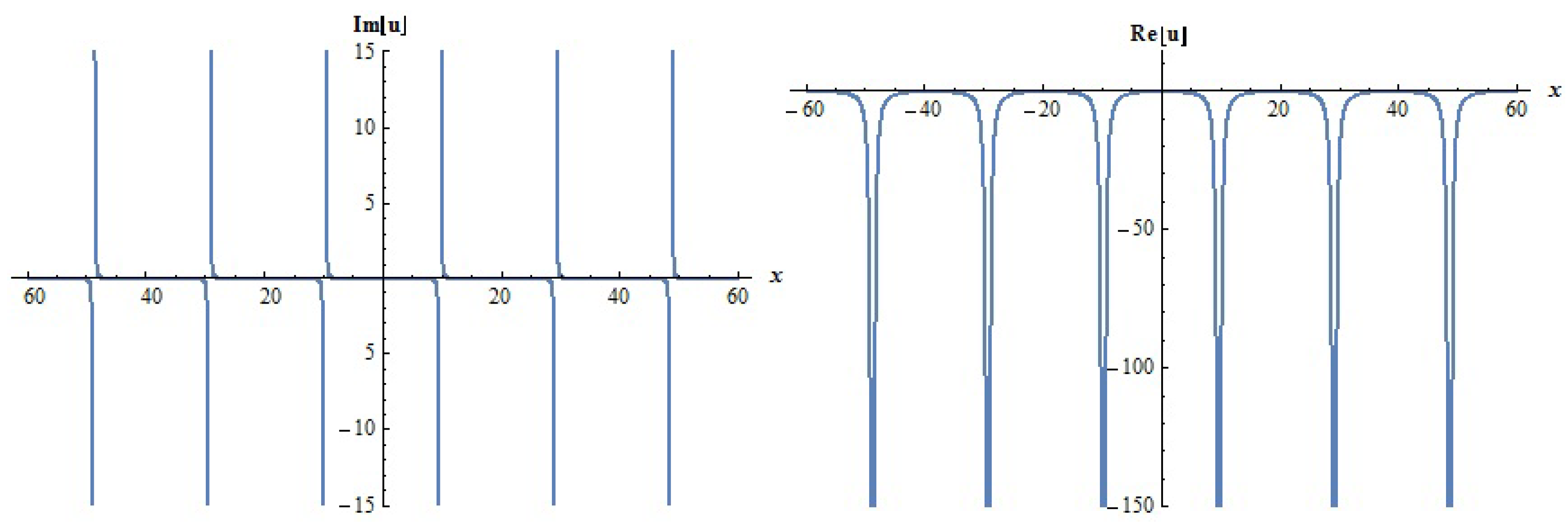
In this section, we apply SGEM to the Equation (1) for obtaining new traveling wave solutions. Applying the traveling wave transformation defined by

$$u(x,y,t)=U\left(\xi \right),\xi =kx+wy-ct,$$

(12)

into Equation (1) results in the following NODE:

$$(c^2-\alpha wc-\alpha w^2+{\alpha }_1ϵkw)U^{{}^{″}}+k^2{\alpha }_2ϵ{\left(U^2\right)}^{{}^{″}}+k^4{ϵ}^2{U}^{\left(4\right)}=0.$$

Integrating twice and setting the integral constants to zero yields the following NODE

$${\alpha }_3{k}^4{ϵ}^2{U}^{{}^{″}}+(c^2-\alpha wc-\alpha w^2+{\alpha }_1ϵkw)U+k^2{\alpha }_2ϵU^2=0.$$

(13)

Balancing in Equation (13) yields $n=2$. Putting $n=2$ in Equation (11), we get the following

$$U\left(w\right)=B_{1}sin\left(w\right)+A_{1}cos\left(w\right)+B_{2}cos\left(w\right)sin\left(w\right)+A_2{cos}^2\left(w\right)+A_0,$$

(14)

and

$$\begin{array}{cc}\hfill U^{{}^{″}}\left(w\right)=& B_1{cos}^2\left(w\right)sin\left(w\right)-B_1{sin}^3\left(w\right)-2A_1{sin}^2\left(w\right)cos\left(w\right)+\hfill \\ \hfill & B_2{cos}^{3}sin\left(w\right)-5B_2{sin}^3\left(w\right)cos\left(w\right)-4A_2{cos}^2\left(w\right){sin}^2\left(w\right)+2A_2{sin}^4\left(w\right).\hfill \end{array}$$

(15)

Substituting Equations (14) and (15) into Equation (13), we obtain an equation of ${sin}^i\left(w\right){cos}^i\left(w\right)$. Getting all coefficients of these terms to zero, we gain a system of equations. Solving this system via some powerful package programs, we find the values of parameters $A_i,B_i,\mu$ and c, which produce many entirely new traveling wave solutions to the Equation (1).

Case-1 When we select these values of parameters as $A_0=\frac{3k^2\epsilon {\alpha }_3}{{\alpha }_2},A_1=0,A_2=-\frac{3k^2\epsilon {\alpha }_3}{{\alpha }_2},B_1=0,B_2=\frac{3i{k}^2\epsilon {\alpha }_3}{{\alpha }_2},c=\frac{1}{2}(\alpha w-\sqrt{\alpha (4+\alpha )w^2-4k\epsilon (w{\alpha }_1+k^3\epsilon {\alpha }_3)})$ for placement into Equation (10) with $n=2$, it yields the following mixed dark-bright soliton solution to the governing model.

$$\begin{array}{cc}\hfill u_1(x,y,t)=& \frac{3k^2\epsilon {\alpha }_3}{{\alpha }_2}+\frac{3i{k}^2\epsilon {\alpha }_3}{{\alpha }_2}\mathrm{sech}(kx+wy-ct)\tanh (kx+wy-ct)\hfill \\ \hfill & -\frac{3k^2\epsilon {\alpha }_3}{{\alpha }_2}{\tanh }^2(kx+wy-ct),\hfill \end{array}$$

(16)

where c is defined as $\frac{1}{2}(\alpha w-\sqrt{\alpha (4+\alpha )w^2-4k\epsilon (w{\alpha }_1+k^3\epsilon {\alpha }_3)})$ with the strain condition $\alpha (4+\alpha )w^2-4k\epsilon (w{\alpha }_1+k^3\epsilon {\alpha }_3)\ge 0$.

Case-2 Choosing as $A_0=\frac{2k^2\epsilon {\alpha }_3}{{\alpha }_2},A_1=0,A_2=-\frac{3k^2\epsilon {\alpha }_3}{{\alpha }_2},B_1=0,B_2=-\frac{3i{k}^2\epsilon {\alpha }_3}{{\alpha }_2},c=\frac{1}{2}(\alpha w+\sqrt{\alpha (4+\alpha )w^2-4k\epsilon w{\alpha }_1+4k^4{\epsilon }^2{\alpha }_3})$ for Equation (10) with $n=2$, it produces another new mixed dark-bright soliton solution as follows.

$$\begin{array}{cc}\hfill u_2(x,y,t)=& \frac{2k^2\epsilon {\alpha }_3}{{\alpha }_2}-\frac{{\alpha }_3}{{\alpha }_2}3i{k}^2\epsilon \mathrm{sech}(kx+wy-ct)\tanh (kx+wy-ct)\hfill \\ \hfill & -\frac{{\alpha }_3}{{\alpha }_2}3k^2\epsilon {\tanh }^2(kx+wy-ct),\hfill \end{array}$$

(17)

where the strain condition is $\alpha w+\sqrt{\alpha (4+\alpha )w^2-4k\epsilon w{\alpha }_1+4k^4{\epsilon }^2{\alpha }_3}\ge 0$.

Case-3 Once we set $A_0=-A_2,A_1=B_1=0,B_2=-i{A}_2,{\alpha }_1=\frac{-3c^2+3\alpha cw+3\alpha w^2+k^2\epsilon A_2{\alpha }_2}{3kw\epsilon },{\alpha }_3=-\frac{A_2{\alpha }_2}{3k^2\epsilon },$ and inserting these values into Equation (10) along with $n=2$, we obtain another new complex dark-bright soliton as follows.

$$\begin{array}{c}\hfill u_3(x,y,t)=-A_2+i{A}_2\mathrm{sech}(-kx-wy+ct)\tanh (-kx-wy+ct)\\ \hfill +A_2{\tanh }^2(-kx-wy+ct);\end{array}$$

(18)

in here, $A_2,k,w,c$ are real constants and non-zero.

Case-4 If it is chosen that $A_0=\frac{6k^2\epsilon {\alpha }_3}{{\alpha }_2},A_1=0,A_2=-\frac{6k^2\epsilon {\alpha }_3}{{\alpha }_2},B_1=0,B_2=0,{\alpha }_1=\frac{-c^2+\alpha cw+\alpha w^2-4k^4{\epsilon }^2{\alpha }_3}{kw\epsilon }$, the dark soliton solution to the Equation (1), when considering Equation (10) to have $n=2$, is obtained as follows.

$$\begin{array}{c}\hfill u_4(x,y,t)=\frac{6k^2\epsilon {\alpha }_3}{{\alpha }_2}(1-{\tanh }^2(-kx-wy+ct)),\end{array}$$

(19)

in which $k,w,c,{\alpha }_3$ are real constants and non-zero.

Case-5 By considering another coefficients defined by $A_0=\frac{-A_2}{3},A_1=B_1=B_2=0,\alpha =\frac{-2A_2^2{\alpha }_2^2+3i{\alpha }_1\sqrt{6}w\sqrt{\epsilon A_2{\alpha }_2{\alpha }_3}+18c^2{\alpha }_3}{18w(c+w){\alpha }_3},k=\frac{i\sqrt{A_2{\alpha }_2}}{\sqrt{6\epsilon {\alpha }_3}}$, we find another complex dark soliton solution given by

$$\begin{array}{c}\hfill u_5(x,y,t)=\frac{-A_2}{3}+A_2{\tanh }^2(\frac{-i\sqrt{A_2{\alpha }_2}}{\sqrt{6\epsilon {\alpha }_3}}x-wy+ct),\end{array}$$

(20)

in which $A_2,\epsilon ,{\alpha }_2,{\alpha }_3,w,c$ are real constants and non-zero.

Case-6 Taking these coefficients as $A_0=-A_2,A_1=B_1=B_2=0,\alpha =\frac{A_2^2{\alpha }_2^2-3i{\alpha }_{1}w\sqrt{1.5\epsilon A_2{\alpha }_2{\alpha }_3}+9c^2{\alpha }_3}{9w(c+w){\alpha }_3},k=\frac{-i\sqrt{A_2{\alpha }_2}}{\sqrt{6\epsilon {\alpha }_3}}$, we find another complex dark soliton solution given by

$$\begin{array}{c}\hfill u_6(x,y,t)=-A_2+A_2{\tanh }^2(\frac{i\sqrt{A_2{\alpha }_2}}{\sqrt{6\epsilon {\alpha }_3}}x-wy+ct),\end{array}$$

(21)

in which $A_2,\epsilon ,{\alpha }_2,{\alpha }_3,w,c$ are real constants and non-zero. Choosing the suitable values of parameters along with strain conditions, we plot some various simulations as being Figure 1, Figure 2, Figure 3, Figure 4, Figure 5, Figure 6, Figure 7 and Figure 8 with the help of computational programs.

4. Conclusions

In this paper, we have successfully applied SGEM into a governing model. Many entirely new soliton solutions, such as dark, mixed dark-bright and complex, have been extracted. Strain conditions have been also given for valid the solutions. By putting suitable values of coefficients in to Equation (10) along with $n=2$, we have plotted the 2D, 3D and contour surfaces of some results. It has been observed that wave patterns from Figure 1, Figure 2, Figure 3, Figure 4, Figure 5, Figure 6, Figure 7 and Figure 8 show their estimated behaviors physically. Moreover, it has been also observed that these results satisfy the considered model. Furthermore, it is also estimated that these dark solitons are related to the gravitational potential [42].

References

1. Wazwaz, A.M. Bright and dark optical solitons for (2+1)-dimensional Schrodinger (NLS) equations in the anomalous dispersion regimes and the normal dispersive regimes. Optik 2019, 192, 162948. [Google Scholar] [CrossRef]
2. Biswas, A.; Yaard, E.; Zhoue, Q.; Seithuti, P.; Belic, M.M. Optical soliton solutions to Fokas-lenells equation using some different methods. Optik 2018, 173, 21–31. [Google Scholar] [CrossRef]
3. Wazwaz, A.M. Multiple complex and multiple real soliton solutions for the integrable sine Gordon equation. Optik 2018, 172, 622–627. [Google Scholar] [CrossRef]
4. Abdullahi, A. Symbolic computation on exact solutions of a coupled KadomtsevPetviashvili equation: Lie symmetry analysis and extended tanh method. Comput. Math. Appl. 2017, 74, 1897–1902. [Google Scholar]
5. Wazwaz, A.M. New (3+1)-dimensional nonlinear evolution equations with mKdV equation constituting its main part: Multiple soliton solutions. Chaos Solitons Fractals 2015, 76, 93–97. [Google Scholar] [CrossRef]
6. Wazwaz, A.M. The tanh method and the sine cosine method for solving the KP-MEW equation. Int. J. Comput. Math. 2007, 82, 235–246. [Google Scholar] [CrossRef]
7. Vakhnenko, V.O.; Parkes, E.J.; Morrison, A.J. A Backlund transformation and the inverse scattering transform method for the generalised Vakhnenko equation. Chaos Solitons Fractals 2003, 17, 683–692. [Google Scholar] [CrossRef]
8. Hu, C.C.; Deng, Y.S.; Tian, B.; Sun, Y.; Zhang, C.R. Rational and semi-rational solutions for the (3+1)-dimensional B-type Kadomtsev Petviashvili Boussinesq equation. Mod. Phys. Lett. B 2019, 33, 1950296. [Google Scholar]
9. Eskitascioglu, E.I.; Aktas, M.B.; Baskonus, H.M. New Complex and Hyperbolic Forms for Ablowitz-Kaup-Newell-Segur Wave Equation with Fourth Order. Appl. Math. Nonlinear Sci. 2019, 4, 105–112. [Google Scholar]
10. Khalique, C.M.; Mhlanga, I.E. Travelling waves and conservation laws of a (2+1)-dimensional coupling system with Korteweg-de Vries equation. Appl. Math. Nonlinear Sci. 2018, 3, 241–254. [Google Scholar] [CrossRef] [Green Version]
11. Bibi, S.; Mohyud-Din, S.T. New traveling wave solutions of Drinfeld Sokolov Wilson Equation using Tanh and Extended Tanh methods. J. Egypt. Math. Soc. 2014, 22, 517–523. [Google Scholar] [CrossRef] [Green Version]
12. Zayed, E.M.; Tala-Tebue, E. New Jacobi elliptic function solutions, solitons and other solutions for the (2+1)-dimensional nonlinear electrical transmission line equation. Eur. Phys. J. Plus 2018, 133, 314. [Google Scholar]
13. Fan, E. Extended tanh-function method and its applications to nonlinear equations. Phys. Lett. A 2000, 277, 212–218. [Google Scholar] [CrossRef]
14. Qingling, G. A Generalized Tanh Method and its Application. Appl. Math. Sci. 2011, 5, 3789–3800. [Google Scholar]
15. Willy, H.; Malfliet, W. The tanh method: II. Perturbation technique for conservative systems. Phys. Scr. 1996, 54, 569–575. [Google Scholar]
16. Zhang, J.L.; Mingliang, X.W. The ( G G ) expansion method and travelling wave solutions of nonlinear evolution equations in mathematical physics. Phys. Lett. A 2008, 372, 417–423. [Google Scholar]
17. Kudryashov, N.A. Traveling wave reduction of the modified KdV hierarchy: The Lax pair and the first integrals. Commun. Nonlinear Sci. Numer. Simul. 2019, 73, 472–480. [Google Scholar] [CrossRef]
18. Kudryashov, N.A. Solitary and periodic waves of the hierarchy for propagation pulse in optical fiber. Optik 2019, 194, 163060. [Google Scholar] [CrossRef]
19. Pandey, P.K. Solution of two point boundary value problems, a numerical approach: Parametric difference method. Appl. Math. Nonlinear Sci. 2018, 3, 649–658. [Google Scholar] [CrossRef] [Green Version]
20. Pandey, P.K.; Jaboob, S.S.A. A finite difference method for a numerical solution of elliptic boundary value problems. Appl. Math. Nonlinear Sci. 2018, 3, 311–320. [Google Scholar] [CrossRef] [Green Version]
21. Raslan, R.K.; Evans, J.D. The tanh function method for solving some important non-linear partial differential equations. Int. J. Comput. Math. 2005, 82, 897–905. [Google Scholar]
22. Raslan, K.R.; Ali, K.K.; Shallal, M.A. The modified extended tanh method with the Riccati equation for solving the space-time fractional EW and MEW equations. Chaos Solitons Fractals 2017, 103, 404409. [Google Scholar] [CrossRef]
23. Zhong, X.; Wu, B.; Sheng, J.; Cheng, K. Generation of bright-dark soliton trains with a central wide dip in optical fibers. Optik 2018, 162, 54–60. [Google Scholar] [CrossRef]
24. Yao, Y.; Ma, G.; Zhang, X.; Liu, W. M-typed dark soliton generation in optical fibers. Optik 2019, 193, 162997. [Google Scholar] [CrossRef]
25. Yao, Y.; Ma, G.; Zhang, X.; Liu, W. Interactions between M-typed dark solitons in nonlinear optics. Optik 2019, 198, 163170. [Google Scholar] [CrossRef]
26. Gao, Y.T.; Tian, B. Generalized hyperbolic-function method with computerized symbolic computation to construct the solitonic solutions to nonlinear equations of mathematical physics. Comput. Phys. Commun. 2001, 133, 158–164. [Google Scholar] [CrossRef]
27. Zhao, Z.; Han, B. Lump solutions of a (3+1)-dimensional B-type KP equation and its dimensionally reduced equations. Anal. Math. Phys. 2019, 9, 119–130. [Google Scholar] [CrossRef]
28. Zhao, Z.; He, L. Multiple lump solutions of the (3+1)-dimensional potential Yu-Toda-Sasa-Fukuyama equation. Appl. Math. Lett. 2019, 95, 114–121. [Google Scholar] [CrossRef]
29. Xu, Z.W.; Yu, G.F.; Zhu, Z.N. Bright-dark soliton solutions of the multi-component AB system. Wave Motion 2018, 83, 134–147. [Google Scholar] [CrossRef] [Green Version]
30. Hirota, R. Exact N-soliton solutions of the wave equation of long waves in shallow water and in nonlinear lattices. J. Math. Phys. 1973, 14, 810–814. [Google Scholar] [CrossRef]
31. Nguyen, L.T.K. Wronskian Formulation and Ansatz Method for Bad Boussinesq Equation. Vietnam J. Math. 2016, 44, 449–462. [Google Scholar] [CrossRef]
32. Nguyen, L.T.K. Soliton Solution of Good Boussinesq Equation. Vietnam J. Math. 2016, 44, 375–385. [Google Scholar] [CrossRef]
33. Xia, L.C.; Ma, W.X.; Liu, X.J.; Zeng, Y.B. Wronskian solutions of the Boussinesq equation solitons, negatons, postions and complexitons. Inverse Probl. 2007, 23, 279–296. [Google Scholar]
34. Nguyen, L.T.K. Modified homogeneous balance method: Applications and new solutions. Chaos Solitons Fractals 2015, 73, 148–155. [Google Scholar] [CrossRef]
35. Tariq, K.U.H.; Seadawy, A.R. Bistable Bright-Dark solitary wave solutions of the (3+1)-dimensional Breaking soliton, Boussinesq equation with dual dispersion and modified Korteweg-de Vries-Kadomtsev-Petviashvili equations and their applications. Results Phys. 2017, 7, 1143–1149. [Google Scholar] [CrossRef]
36. Cao, Y.; He, J.; Mihalache, D. Families of exact solutions of a new extended (2+1)-dimensional Boussinesq equation. Nonlinear Dyn. 2018, 91, 2593–2605. [Google Scholar] [CrossRef]
37. Moleleki, L.D.; Khalique, C.M. Solutions and Conservation Laws of a (2+1)-Dimensional Boussinesq Equation. Abstr. Appl. Anal. 2003, 2013, 1–8. [Google Scholar] [CrossRef] [Green Version]
38. Lu, D.; Seadawy, A.R.; Ahmed, I. Applications of mixed lump-solitons solutions and multi-peaks solitons for newly extended (2+1)-dimensional Boussinesq wave equation. Mod. Phys. Lett. B 2019, 33, 1950363. [Google Scholar] [CrossRef]
39. Gao, W.; Ismael, H.F.; Husien, A.M.; Bulut, H.; Baskonus, H.M. Optical Soliton solutions of the Nonlinear Schrödinger and Resonant Nonlinear Schrödinger Equation with Parabolic Law. Appl. Sci. 2020, 10, 219. [Google Scholar] [CrossRef] [Green Version]
40. Guirao, J.L.G.; Baskonus, H.M.; Kumar, A.; Rawat, M.S.; Yel, G. Complex Soliton Solutions to the (3+1)-Dimensional B-type Kadomtsev-Petviashvili-Boussinesq Equation. Symmetry 2020, 12, 17. [Google Scholar] [CrossRef] [Green Version]
41. Ismael, H.F.; Bulut, H.; Baskonus, H.M. Optical soliton solutions to the Fokas-Lenells equation via sine-Gordon expansion method and (m+G’/G)-expansion method. Pramana J. Phys. 2020, 94, 35. [Google Scholar] [CrossRef]
42. Weisstein, E.W. Concise Encyclopedia of Mathematics, 2nd ed.; CRC: New York, NY, USA, 2002. [Google Scholar]
Figure 1. The 3D figures of u 1 for k = 0.1, w = 2, ε = 1, α = 0.4 , α 1 = 0.3, α 2 = 4, α 3 = 0.5, y = 0.05.
Mathematics 08 00341 g001
Figure 2. The contour simulations of u 1 for k = 0.1, w = 2, ε = 1, α = 0.4 , α 1 = 0.3, α 2 = 4, α 3 = 0.5, y = 0.05.
Mathematics 08 00341 g002
Figure 3. The 3D figures of u 5 for α 2 = 0.1, α 3 = 0.32, ε = 1, w = 0.012 , A 2 = 0.2 , c = 0.3, y = 0.05.
Mathematics 08 00341 g003
Figure 4. The contour simulations of u 5 for α 2 = 0.1, α 3 = 0.32, ε = 1, w = 0.012 , A 2 = 0.2 , c = 0.3, y = 0.05.
Mathematics 08 00341 g004
Figure 5. The 2D graphs of u 5 for α 2 = 0.1, α 3 = 0.32, ε = 1, w = 0.012 , A 2 = 0.2 , c = 0.3, t = 0.13, y = 0.05.
Mathematics 08 00341 g005
Figure 6. The 3D figures of u 6 for α 2 = 0.1, α 3 = 0.32, ε = 1, w = 0.012 , A 2 = 0.5 , c = 0.01, y = 0.05.
Mathematics 08 00341 g006
Figure 7. The contour simulations of u 6 for α 2 = 0.1, α 3 = 0.32, ε = 1, w = 0.012 , A 2 = 0.5 , c = 0.01, y = 0.05.
Mathematics 08 00341 g007
Figure 8. The 2D graphs of u 6 for α 2 = 0.1, α 3 = 0.32, ε = 1, w = 0.012 , A 2 = 0.5 , c = 0.01, t = 0.01, y = 0.05.
Mathematics 08 00341 g008