An Integrated Approach of Best-Worst Method (BWM) and Triangular Fuzzy Sets for Evaluating Driver Behavior Factors Related to Road Safety

Abstract

Driver behavior plays a major role in road safety because it is considered as a significant argument in traffic accident avoidance. Drivers mostly face various risky driving factors which lead to fatal accidents or serious injury. This study aims to evaluate and prioritize the significant driver behavior factors related to road safety. In this regard, we integrated a decision-making model of the Best-Worst Method (BWM) with the triangular fuzzy sets as a solution for optimizing our complex decision-making problem, which is associated with uncertainty and ambiguity. Driving characteristics are different in different driving situations which indicate the ambiguous and complex attitude of individuals, and decision-makers (DMs) need to improve the reliability of the decision. Since the crisp values of factors may be inadequate to model the real-world problem considering the vagueness and the ambiguity, and providing the pairwise comparisons with the requirement of less compared data, the BWM integrated with triangular fuzzy sets is used in the study to evaluate risky driver behavior factors for a designed three-level hierarchical structure. The model results provide the most significant driver behavior factors that influence road safety for each level based on evaluator responses on the Driver Behavior Questionnaire (DBQ). Moreover, the model generates a more consistent decision process by the new consistency ratio of F-BWM. An adaptable application process from the model is also generated for future attempts.

1. Introduction

According to data from the worldwide road safety status report, annual traffic deaths are reported to reach 1.35 million [1]. According to this report, it was stated that the road safety performance for Hungary is below the EU average. In 2018, the proportion of people died on the roads in Hungary was set at 64 per million, and this statistic increased by 1% compared to the previous year [2]. However, the Road Safety Action Program (2014–2016) was integrated with the Hungarian Transport Strategy in line with the goal of reducing the number of road deaths by 50% between 2010 and 2020. According to the Road Safety Action Program situation analysis, most accidents stemmed from human-induced factors. Therefore, addressing them becomes a dynamic target of road safety actions [3]. According to the estimates of some previous studies, approximately 90% of road traffic accidents have been found to be the sole or major causative factor of human factors [4,5,6].

Many driver behavior factors emerge as dynamic, deliberate violations of the rules and mistakes resulting from less driving experience, while others appear as a result of carelessness, momentary errors, or failure to perform an action, the latter being generally age-related [7,8]. In order to alleviate the driver’s workload and increase the basic services of active vehicle safety systems, identification of risky driver behavior factors has been handled. However, these systems based on the average driver performance on the road and individual driver’s attitudes were seldom taken into consideration [9].

To analyze the risky driving behavior for road safety, the Driver Behavior Questionnaire (DBQ) was first introduced as a tool in the studies in the 1990s [10,11]. Reason et al., (1990) detected three kinds of driving behaviors, i.e., errors, lapses, and violations, and analyzed the association between driving behavior and accident involvement. Accordingly, human error is an unintended act or decision. Slips and lapses happen in very familiar tasks that we can execute without very much conscious consideration. Violations are intended failures—intentionally doing the wrong act [12,13,14]. In addition, the Driver Behavior Questionnaire (DBQ), with an extended version, was used to evaluate aberrant driver behaviors [12]. While the extended version of the DBQ consists of aggressive and ordinary violations, lapses and errors [14]. An aggressive violation behavior was identified as contradictory behavior towards other road users [13].

The previous study observed that the analytic hierarchy process (AHP) method was an effective approach in terms of prioritizing suburban road safety indicator to access the factors which reduce the number and severity of accidents in Iran [15]. However, the prioritizing of the AHP method is rather imprecise; and the subjective assessment by perception, evaluation, development, and assortment based on the preference of decision-makers (DMs) have a significant impact on AHP outcomes [16]. To deal with such tricky problems, many researchers integrate fuzzy theory with AHP to incorporate its results [17,18,19,20,21]. The fuzzy AHP, compared to AHP and the statistical methods of prioritization, has greater precision and certainty. Although in AHP, the experts compare the alternatives using their competencies and intellectual skills, but it may not completely reflect the human thinking style. However, the use of fuzzy numbers is more consistent in human linguistic representations. Therefore, the decisions can be made more reliable and more precise in the real world using fuzzy numbers [22].

However, it is not possible to ignore the inconsistency in AHP-based pairwise comparison matrices (PCMs) because inconsistency often occurs in practice [23,24]. The inconsistency in PCMs is the main drawback of AHP and can lead to uncertain results. In general, it is obvious that if the PCM is 5 × 5 or larger in the decision structure, the relatively consistent filling of this size of matrix by non-expert evaluators requires significant effort [16].

In order to solve this consistency problem in traditional AHP and to minimize PC surveys, Rezaei introduced the BWM method [25] to reduce the number of pairwise comparisons in the traditional AHP process. As a new technique, there are still gaps in both the theoretical structure and application areas of BWM. Thus, some questions remained open in terms of conditions and limitations on traditional AHP usage. For the BWM itself, the appropriate consistency ratio value and the inconsistency improving procedures can be addressed. Additionally, the BWM within other contexts could investigate the uncertainty. The model’s multiple optimality solution in BWM can be determined from other angles [26].

Due to the statistic that BWM is sensitive to preferences of DMs, it is very complicated to calculate the accurate weights when the DM utilizes natural language, such as “very high”, “medium”, or “very low”, to express a type of overall preferences [27]. Therefore, in this study, the crisp preferences in BMW are stretched with triangular fuzzy numbers to overcome the inherent ambiguity of the DM’s decision in real decision-making problems. Furthermore, this F-BWM model gives fewer PCs with high consistency of the pairwise comparison matrix. Saaty explains that consistency will not be good when the number of factors exceeds 7 ± 2 [28]. This is also a theoretical justification of Miller’s psychological investigation [29]. Therefore, the proposed model produces more consistent and reliable results with fewer PCs. In summary, BWM with triangular fuzzy sets merely considers reference pairwise comparisons and handles inconsistency in an effective manner versus conventional AHP with triangular fuzzy sets. Therefore, it presents an easy and accurate decision framework.

2. Literature Review

In the literature, BWM and its fuzzy extended versions are frequently applied to various areas, from manufacturing to supply chain management and transportation [30]. Although plenty of papers have been published in these areas, there are very few contributions applied to the evaluation of driving behaviors for road safety. Most of the recent BWM/F-BWM contributions focus on supply chain design, supplier or green supplier evaluation, and occupational or environmental safety risk analysis [31].

Regarding supply chain performance and supplier assessment, Badi and Ballem [31] studied supplier selection problems in the pharmaceutical industry using an integrated rough BWM method. While the Z-number BWM is proposed by Aboutorab et al. [32] for supplier development problem, intuitionistic F-BWM is applied for the green supplier selection problem by Tian et al. [33]. Wu et al. [34] integrated the interval type-2 fuzzy sets and BWM for green supplier selection problems.

In the risk assessment literature, AHP or F-AHP is mostly used as a weighted factor scoring method for risk parameters. After BWM is introduced, researchers have begun to use it instead of AHP due to its superiorities. BWM/F-BWM is used to assign weights to risk parameters like AHP. In many studies, it is frequently integrated with FMEA [35,36,37,38,39,40]. In some other studies, it is integrated with MCDM such as interval triangular fuzzy Delphi method under 5 × 5 matrix [41], F-TOPSIS [42], and artificial intelligence-based methods such as Bayesian networks [43,44] and business impact analysis [45].

In the light of this brief review of the previous studies related to BWM and F-BWM applied to diverse selection and ranking problems, it is observed that BWM has not integrated yet with fuzzy sets for the addressed problem “driving behavior evaluation”. Therefore, in the proposed approach, F-BWM is utilized to determine the importance weight of driver behavior factors related to road safety. As fuzzy extensions, triangular fuzzy numbers are used in the existed study since they reflect uncertainty in the decision-making process well. Additionally, the DBQ is attached to the F-BWM to strengthen the methodology of the study. The benefits of the applied F-BWM methodology are as follows: (1) From the theoretical viewpoint, it has designed a solid decision-making framework with the aid of triangular fuzzy numbers and, modeled uncertainty well. Although the literature covers methods like AHP and BWM in determining the importance weights of factors, the F-BWM methodology fits well with the structure of the problem handled in this study. The full consistency method (FUCOM) is the simplest example. It is proposed by Pamučar et al. [46] and applied by many scholars [47,48,49] to various MCDM problems. (2) From an application viewpoint, the study considers a DBQ and priorities the driving behavior factors relating to road safety. Previous studies regarding driving behavior factor evaluation are mostly based on statistical inference logic either cross-sectional or cross-cultural. However, this study handles the problem in an MCDM manner. Additionally, as a case study, the Budapest city of Hungary is studied to demonstrate applicability. Of course, the approach can be adapted to other cities.

3. Materials and Methods

3.1. Driver Behavior Questionnaire (DBQ) Survey

The study utilized the driver behavior questionnaire (DBQ) as a tool to collect driver behavior data on perceived road safety issues from Budapest city. To do so, the car drivers having at least fifteen-year driving experience were asked to fill the DBQ by face-to-face method, which increased its reliability. The drivers who participated in this study were the faculty members of the Department of Transport Technology and Economics and the Department of Control for Transportation and Vehicle Systems at Budapest University of Technology and Economics who also have transportation engineering research experience. In addition, the participants were asked to indicate how often they likely to involve in each of the observed driver behaviors in the recent year using Saaty’s traditional ratio scale (1–9). The questionnaire survey was designed in two parts: The first part intended to measure demographic data about the participants and results are tabulated in

Table 1. Sample characteristics.

Variables	Data Analysis Results
N	100
Age: Mean (SD)	32.341 (3.421)
Gender (1 = male, 0 = female): Mean (SD)	0.845 (0.125)
Duration of driving license: Mean (SD)	15.312 (1.589)

. The results stated the mean and standard deviation (SD) values of observed data such as age, gender, and driving experience based on drivers’ responses. In addition, we used digits (1, 0) for assessment purposes to explain simply the characteristics of gender.

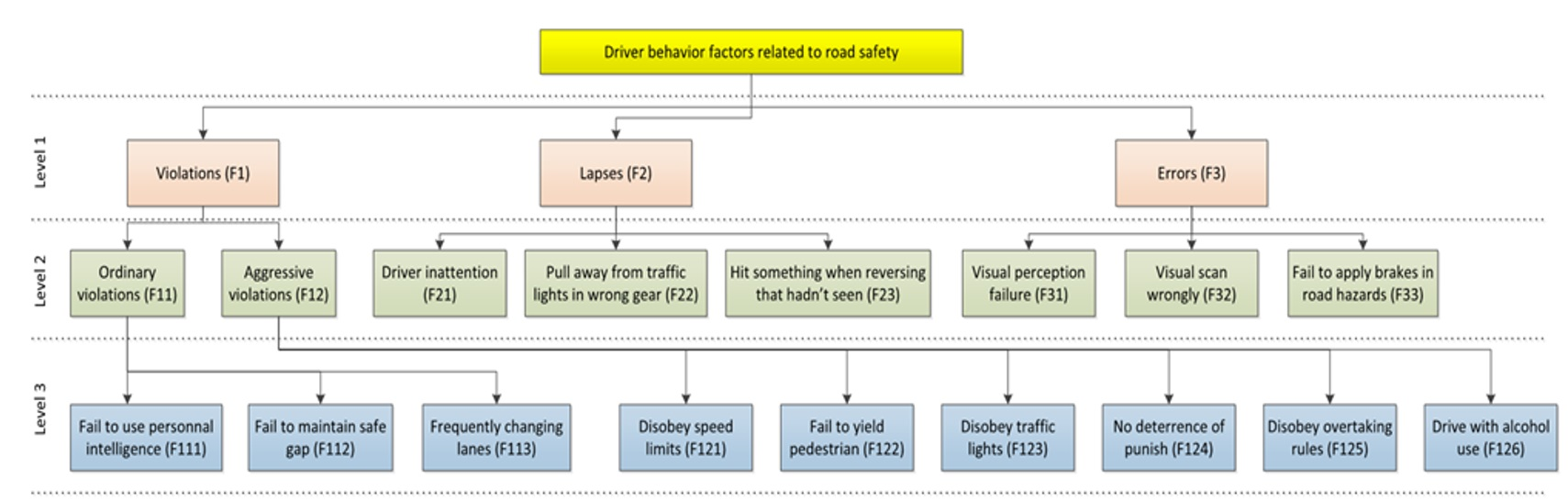
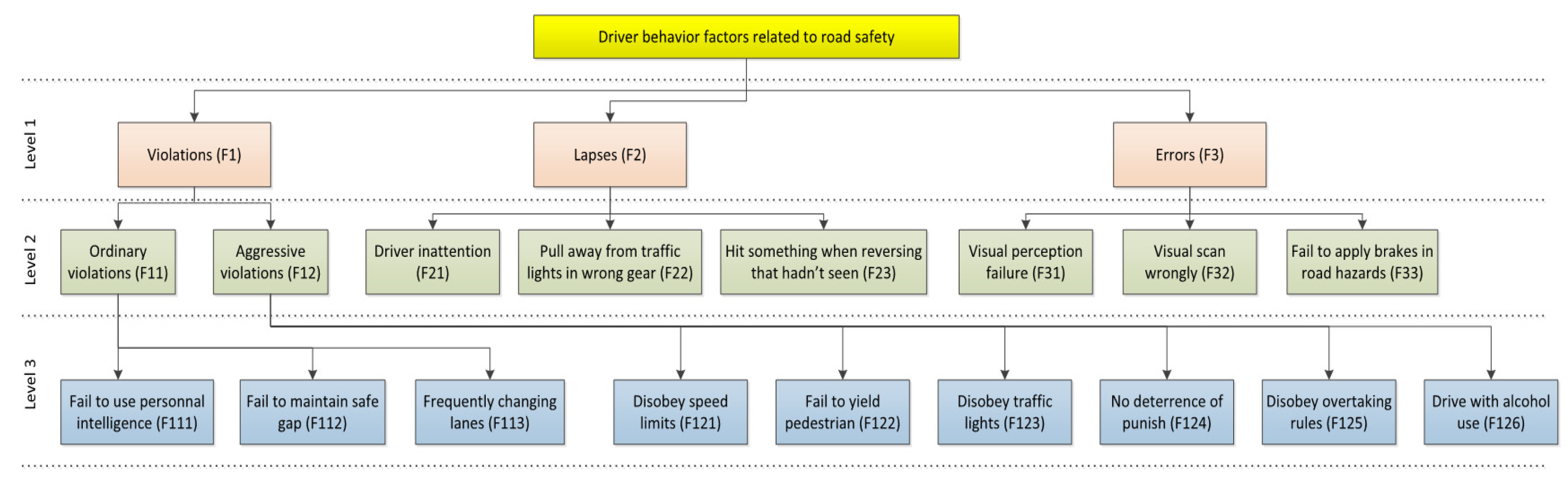
The second part of DBQ designed on Saaty scale (1977) to analyze the significant driver behavior factors related to road safety. For evaluation purposes, the driver behavior factors were designed in a three-level hierarchical structure and symbolized each factor with alphabet ‘F’ as shown in Figure 1. These driver behavior factors have a significant influence on road safety. Some recent studies considered the specified driver behavior factors for evaluation of road safety performance by different evaluator groups [50,51,52].

3.2. Overview on Best Worst Method (BWM)

The general BWM method was created by Rezaei (2015) to derive the weights of the criteria with the smaller number of comparisons and more consistent comparisons. The most important factor is the one which has the most vital role in making the decision, while the less important has the opposite role in the decision process. Furthermore, the BMW does not only derive the weights independently but it can also be combined with other multi-criteria-decision-making methods [53,54,55].

• The procedure of the BWM can be highlighted as follows:
• Identification of the decision-making problem and its factors
• Determination of the most crucial and least crucial factor
• Determination of the preference of the most crucial factor over all the other factors
• Determination of the preference of the least crucial factor over all the other factors
• Make the consistency check
• Determination of the importance weight of the factors

We consider a set of elements ($e_1,e_2,\dots ,e_n$) and then select the most important element and compare it to others using Saaty’s scale (1–9). Accordingly, this provides the most important element to other vectors would be: $E_a=\left(e_{a1},e_{a2},\dots ,e_{an}\right)$, and obviously $e_{aa}=1$. However, the least important element to other vectors would be: $E_b={\left(e_{1b},e_{2b},\dots ,e_{nb}\right)}^T$ by using the same scale.

After deriving the optimal weight scores, the consistency has been checked through computing the consistency ratio from the following formula:

$$\begin{gathered} {\xi }^2-(1+2u_{BW})\xi +(u_{BW}^2-u_{BW})=0 \\ ConsistencyRatio=\frac{{\xi }^{*}}{ConsistencyIndex} \end{gathered}$$

(1)

where

Table 2. Consistency index (CI) values.

${\mathit{e}}_{\mathit{a}\mathit{b}}$	1	2	3	4	5	6	7	8	9
$ConsistencyIndex\left(\max \xi \right)$	0.0	0.44	1.0	1.63	2.3	3.0	3.73	4.47	5.23

provides us the consistency index values:

To obtain an optimal weight for all elements, the maximum definite differences are $\left|\frac{w_a}{w_j}-e_{aj}\right|$ and $\left|\frac{w_j}{w_b}-e_{jb}\right|$, and for all $j$ is minimized. If we assumed a positive-sum for the weights, the following problem would be solved:

$$\begin{array}{l}\min ma{x}_j\left\{\left|\frac{w_a}{w_j}-e_{aj}\right|,\left|\frac{w_j}{w_b}-e_{jb}\right|\right\}\\ \mathrm{s}.\mathrm{t}.\\ {\displaystyle \sum }_j{b}_j=1\\ b_j\ge 0,\mathrm{for}\mathrm{all}j\end{array}$$

(2)

The problem could be transferred into the following problem:

$$\begin{array}{l}\min \xi \\ \mathrm{s}.\mathrm{t}.\\ \left|\frac{w_a}{w_j}-e_{aj}\right|\le \xi ,\mathrm{for}\mathrm{all}j\\ \left|\frac{w_j}{w_b}-e_{jb}\right|\le \xi \mathrm{for}\mathrm{all}j\\ {\displaystyle \sum }_j{b}_j=1\\ b_j\ge 0,\mathrm{for}\mathrm{all}j\end{array}$$

(3)

By solving this problem, we obtain the optimal weights and ${\xi }^{*}$. For further reading on priority criteria, one may refer to [56,57]. While $w_B$ presents the importance weights of best criterion, $w_W$ shows the e importance weights of the worst criterion. $e_{Bj}$ denotes the evaluation of the best to others, $e_{Wj}$ denotes the evaluation of the others to worst.

3.3. The Proposed F-BWM Model

3.3.1. General Information on Fuzzy Sets

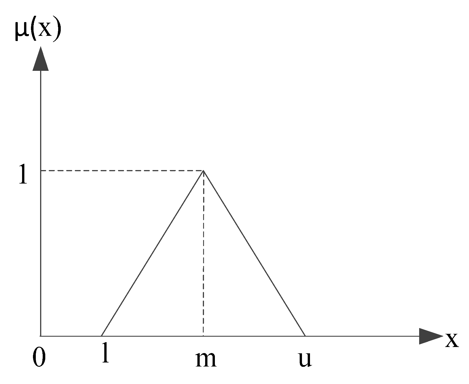
Prior to explaining F-BWM, some fundamental notations regarding fuzzy sets can be useful. Zadeh [58] introduced fuzzy sets for better reflecting of the human judgments and assessment in the decision making process. It is considered as a more robust tool to deal with vagueness, ambiguity, and uncertainty. Many decision-making problems consist of goals, constraints, and possible actions that are not known precisely [58]. The usage of fuzzy sets is better for transforming the linguistic decision of human judgment. Hence, many real-world decision-making problems have used fuzzy sets [59,60]. A triangular fuzzy number consists of lower, medium and upper numbers of the fuzzy as $\tilde{A}=\left(l,m,u\right)$ where l, m and u which is crisp and real numbers ($x\le y\le z.$ The membership function of a triangular fuzzy number can be defined as follows:

$${\mu }_{\tilde{A}}=\{\begin{array}{cc}0,& x<l\\ \left(x-l\right)/\left(m-l\right),& l\le x\le m\\ \left(u-x\right)/\left(u-m\right),& m\le x\le u\\ 0& x\ge u\end{array}$$

(4)

A triangular fuzzy number is presented in Figure 2. The linguistic terms and triangular fuzzy numbers are also given in

Table 3. The linguistic terms and fuzzy numbers.

Linguistic Term	Triangular Fuzzy Number
Equally Importance (EI)	(1, 1, 1)
Weakly Important (WI)	(2/3, 1, 1.5)
Fairly Important (FI)	(1.5, 2, 2.5)
Very Important (VI)	(2.5, 3, 3.5)
Absolutely Important (AI)	(3.5, 4, 4.5)

.

${\tilde{A}}_1=\left(l_1,m_1,u_1\right)$ and ${\tilde{A}}_2=\left(l_2,m_2,u_2\right)$ are any two triangular fuzzy numbers, and the mathematical calculation of the two triangular fuzzy numbers is defined as follows:

The addition operation:

$${\tilde{A}}_1+{\tilde{A}}_2=\left(l_1+l_2,m_1+m_2,u_1+u_2\right)$$

(5)

The subtraction operation:

$${\tilde{A}}_1-{\tilde{A}}_2=\left(l_1-u_2,m_1-m_2,u_1-l_2\right)$$

(6)

The multiplication operation:

$${\tilde{A}}_{1}x{\tilde{A}}_2=\left(l_{1}x{l}_2,m_{1}x{m}_2,u_{1}x{u}_2\right)$$

(7)

The arithmetic operation:

$$kx{\tilde{A}}_1=\left(kx{l}_1,kx{m}_1,kx{u}_1\right),\left(k>0\right)$$

(8)

$$\frac{{\tilde{A}}_1}{k}=\left(\frac{l_1}{k},\frac{m_1}{k},\frac{u_1}{k}\right),\left(k>0\right)$$

(9)

The graded mean integration representation (GMIR) $R\left({\tilde{A}}_i\right)$ of a triangular fuzzy number for the ranking of triangular fuzzy number is calculate as follows:

$$R\left({\tilde{A}}_i\right)=\frac{l_i+4m_i+u_i}{6}$$

(10)

3.3.2. Fuzzy Best-Worst Method (F-BWM)

The BWM was proposed by Rezai (2015) for multi-criteria decision-making problems considering pairwise comparison manner. The best and worst criteria are determined in BWM [33]. Different fuzzy sets-based versions have been proposed as intuitionistic fuzzy sets [32,61], triangular fuzzy numbers [27,62], Z-numbers [34], dominance degree [63], and interval type-2 fuzzy number [64,65]. Mi et al. [66] presented a survey of BWM applications and extensions. The interested readers and researchers may refer to this study in detail.

In BWM, there are $n$ criteria, and the fuzzy pairwise comparisons are applied based on the linguistic terms of decision-makers as presented in Table 3. Then, the linguistic evaluations are transformed into triangular fuzzy numbers. The fuzzy comparison matrix is getting as follows:

$$\begin{array}{ll}& \begin{array}{cccc}{c}_1& c_2& \cdots & c_n\end{array}\\ \tilde{A}=\begin{array}{c}{c}_1\\ c_2\\ ⋮\\ c_n\end{array}& \left[\begin{array}{cccc}{\tilde{a}}_{11}& {\tilde{a}}_{12}& \cdots & {\tilde{a}}_{1n}\\ {\tilde{a}}_{21}& {\tilde{a}}_{22}& \cdots & {\tilde{a}}_{2n}\\ ⋮& ⋮& \ddots & ⋮\\ {\tilde{a}}_{n1}& {\tilde{a}}_{n2}& \cdots & {\tilde{a}}_{nn}\end{array}\right]\end{array}$$

where ${\tilde{a}}_{ij}$ denotes the relative fuzzy preference of criterion i to criterion j, which is a triangular fuzzy number; ${\tilde{a}}_{ij}=\left(1,1,1\right)$ when i = j.

In this paper, we will present the detailed steps of fuzzy BWM. The detailed steps of fuzzy BWM are used for obtaining the fuzzy weights [62].

Step 1. Construct the criteria system. A set of criteria reflects the performances of different criteria. Suppose there are n decision criteria $\left\{c_1,c_2,\dots ,c_n\right\}$.

Step 2. Determine the best criterion and the worst criterion. In this step, the best criterion and the worst criterion is determined by experts based on the constructed decision criteria system. The best criterion is denoted as $c_B$, and the worst criterion is also denoted as $c_W$.

Step 3. Perform the fuzzy reference comparisons for the best criterion. According to the pairwise comparison ${\tilde{a}}_{ij}$, $c_B$ is the best criterion; $c_W$ is the worst criterion. The fuzzy preferences of the best criterion over all the criteria can be determined. Then, the fuzzy comparisons are converted to triangular fuzzy numbers. The fuzzy Best-to-Others vector is obtained as follows:

$${\tilde{A}}_B=\left\{{\tilde{a}}_{B1},{\tilde{a}}_{B2},\dots ,{\tilde{a}}_{Bn}\right\}$$

where ${\tilde{A}}_B$ denotes the fuzzy best-to-others vector; ${\tilde{a}}_{Bj}$ denotes the fuzzy comparison of the best criterion $c_B$ over criterion j, $j=1,2,\dots ,n$. It is known that ${\tilde{a}}_{BB}=\left(1,1,1\right)$.

Step 4. Perform the fuzzy reference comparisons for the worst criterion. In this step, the fuzzy preferences of all the criteria over the worst criterion can be determined. They are transformed into triangular fuzzy numbers. The fuzzy others-to-worst vector can be obtained as:

$${\tilde{A}}_W=\left\{{\tilde{a}}_{1W},{\tilde{a}}_{2W},\dots ,{\tilde{a}}_{nW}\right\}$$

where ${\tilde{A}}_W$ denotes the fuzzy others-to-worst vector; ${\tilde{a}}_{iW}$ denotes the fuzzy comparison of the worst criterion $c_W$, $i=1,2,\dots ,n$. It is known that ${\tilde{a}}_{WW}=\left(1,1,1\right)$.

Step 5. Determine the optimal fuzzy weights$\left({\tilde{w}}_1^{*},{\tilde{w}}_2^{*},\dots ,{\tilde{w}}_n^{*}\right)$. In this step, the optimal fuzzy weight for each criterion is determined for each fuzzy pair ${\tilde{w}}_B/{\tilde{w}}_j$ and ${\tilde{w}}_j/{\tilde{w}}_W$. It should have ${\tilde{w}}_B/{\tilde{w}}_j={\tilde{a}}_{Bj}$ and ${\tilde{w}}_j/{\tilde{w}}_W={\tilde{a}}_{jW}$. A solution is obtained that the maximum absolute gaps $\left|\frac{{\tilde{w}}_B}{{\tilde{w}}_j}-{\tilde{a}}_{Bj}\right|$ and $\left|\frac{{\tilde{w}}_j}{{\tilde{w}}_W}-{\tilde{a}}_{jW}\right|$ for all j are minimized to satisfy these conditions for all j. ${\tilde{w}}_B$,${\tilde{w}}_j$ and ${\tilde{w}}_W$ in fuzzy BWM are triangular fuzzy numbers. In some cases, we prefer to use ${\tilde{w}}_j=\left(l_j^w,m_j^w,u_j^w\right)$ for optimal criteria selection. The triangular fuzzy weight of the criterion ${\tilde{w}}_j=\left(l_j^w,m_j^w,u_j^w\right)$ is transformed to a crisp value using Equation (11). Consequently, the constrained optimization problem is constructed for obtaining the optimal fuzzy weights $\left({\tilde{w}}_1^{*},{\tilde{w}}_2^{*},\dots ,{\tilde{w}}_n^{*}\right)$ as follows:

$$\begin{array}{l}\min \underset{j}{\max }\left\{\left|\frac{{\tilde{w}}_B}{{\tilde{w}}_j}-{\tilde{a}}_{Bj}\right|,\left|\frac{{\tilde{w}}_j}{{\tilde{w}}_W}-{\tilde{a}}_{jW}\right|\right\}\\ s.t.\{\begin{array}{l}{\displaystyle \sum _{j=1}^{n}R\left({\tilde{w}}_i\right)}=1\\ l_j^w\le m_j^w\le u_j^w\\ l_j^w\ge 0\\ j=1,2,\dots ,n\end{array}\end{array}$$

(11)

where ${\tilde{w}}_B=\left(l_B^w,m_B^w,u_B^w\right)$, ${\tilde{w}}_j=\left(l_j^w,m_j^w,u_j^w\right)$, ${\tilde{w}}_W=\left(l_W^w,m_W^w,u_W^w\right)$, ${\tilde{a}}_{Bj}=\left(l_{Bj}^w,m_{Bj}^w,u_{Bj}^w\right)$ and ${\tilde{a}}_{jW}=\left(l_{jW}^w,m_{jW}^w,u_{jW}^w\right)$. Equation (12) is transformed to the nonlinearly constrained optimization problem:

$$\begin{array}{l}\min \xi \\ s.t.\{\begin{array}{l}\left|\frac{{\tilde{w}}_B}{{\tilde{w}}_j}-{\tilde{a}}_{Bj}\right|\le \xi \\ \left|\frac{{\tilde{w}}_j}{{\tilde{w}}_W}-{\tilde{a}}_{jW}\right|\le \xi \\ {\displaystyle \sum _{j=1}^{n}R\left({\tilde{w}}_i\right)}=1\\ l_j^w\le m_j^w\le u_j^w\\ l_j^w\ge 0\\ j=1,2,\dots ,n\end{array}\end{array}$$

(12)

where $\xi =\left(l^{\xi },m^{\xi },u^{\xi }\right)$.

Considering $l^{\xi }\le m^{\xi }\le u^{\xi }$, it is supposed that ${\xi }^{*}=\left(k^{*},k^{*},k^{*}\right)$, $k^{*}\le l^{\xi }$ then Equation (13) can be transferred as:

$$\begin{array}{l}\min {\xi }^{*}\\ s.t.\{\begin{array}{l}\left|\frac{\left(l_B^w,m_B^w,u_B^w\right)}{\left(l_j^w,m_j^w,u_j^w\right)}-\left(l_{Bj},m_{Bj},u_{Bj}\right)\right|\le \left(k^{*},k^{*},k^{*}\right)\\ \left|\frac{\left(l_j^w,m_j^w,u_j^w\right)}{\left(l_W^w,m_W^w,u_W^w\right)}-\left(l_{jW},m_{jW},u_{jW}\right)\right|\le \left(k^{*},k^{*},k^{*}\right)\\ {\displaystyle \sum _{j=1}^{n}R\left({\tilde{w}}_i\right)}=1\\ l_j^w\le m_j^w\le u_j^w\\ l_j^w\ge 0\\ j=1,2,\dots ,n\end{array}\end{array}$$

(13)

Step 6. Determine the consistency ratio. The consistency ratio is determined in the same way as BWM. In this step, the consistency index for fuzzy BWM is calculated.

The main steps of the proposed F-BWM model are discussed in Figure 3.

4. Results

The F-BWM model was applied to evaluate driver behavior factors related to road safety and to compute weight scores. Furthermore, the reliability of the PCs consistency in F-BWM was checked, and it was acceptable for each matrix. In the following, step by step application of F-BWM to the problem is provided. In this application, three main factors, eight sub-factors, and nine sub-sub-factors are evaluated. We will first present the F-BWM model for main factors as violations (F₁), lapses (F₂), and errors (F₃). The violations (F₁) and lapses (F₂) are determined as the most significant and the less significant factor, respectively (Step 2). The fuzzy reference comparisons are applied, and the linguistic terms for fuzzy preferences of the most significant factor and the less significant factor are given in

Table 4. The linguistic terms for fuzzy preferences of the most important factor.

Factor	F1	F2	F3
Best factor (F1)	EI	FI	WI

and

Table 5. The linguistic terms for fuzzy preferences of the less important factor.

Factor	Worst Factor (F2)
F1	FI
F2	EI
F3	WI

, respectively.

Then, the fuzzy most significant-to-others vector and the fuzzy others-to-less significant can be obtained with respect to Table 3 as follows (Step 3).

$$\begin{gathered} {\tilde{a}}_B=\left[(1,1,1),(3/2,2,5/2),(2/3,1,3/2)\right] \\ {\tilde{a}}_W=\left[(3/2,2,5/2),(1,1,1),(2/3,1,3/2)\right] \end{gathered}$$

Then, for obtaining the optimal fuzzy weights of all the main factors, the nonlinearly constrained model is constructed as follows in Equation (14):

$$\begin{array}{l}\min {\xi }^{*}\\ s.t.\{\begin{array}{l}\left|\frac{\left(l_{f1}^w,m_{f1}^w,u_{f1}^w\right)}{\left(l_{f1}^w,m_{f1}^w,u_{f1}^w\right)}-\left(l_{f11},m_{f11},u_{f11}\right)\right|\le (e^{*},e^{*},e^{*})\\ \left|\frac{\left(l_{f1}^w,m_{f1}^w,u_{f1}^w\right)}{\left(l_{f2}^w,m_{f2}^w,u_{f2}^w\right)}-\left(l_{f12},m_{f12},u_{f1\left|\right|2}\right)\right|\le (e^{*},e^{*},e^{*})\\ \left|\frac{\left(l_{f1}^w,m_{f1}^w,u_{f1}^w\right)}{\left(l_{f3}^w,m_{f3}^w,u_{f3}^w\right)}-\left(l_{f13},m_{f13},u_{f13}\right)\right|\le (e^{*},e^{*},e^{*})\\ \left|\frac{\left(l_{f1}^w,m_{f1}^w,u_{f1}^w\right)}{\left(l_{f2}^w,m_{f2}^w,u_{f2}^w\right)}-\left(l_{f12},m_{f12},u_{f12}\right)\right|\le (e^{*},e^{*},e^{*})\\ \left|\frac{\left(l_{f2}^w,m_{f2}^w,u_{f2}^w\right)}{\left(l_{f2}^w,m_{f2}^w,u_{f2}^w\right)}-\left(l_{f22},m_{f22},u_{f22}\right)\right|\le (e^{*},e^{*},e^{*})\\ \left|\frac{\left(l_{f3}^w,m_{f3}^w,u_{f3}^w\right)}{\left(l_{f2}^w,m_{f2}^w,u_{f2}^w\right)}-\left(l_{f32},m_{f32},u_{f32}\right)\right|\le (e^{*},e^{*},e^{*})\\ {\displaystyle \sum _{j=1}^{3}R({\tilde{w}}_j)=1}\\ l_{fj}^w\le m_{fj}^w\le u_{fj}^w\\ l_{fj}^w\ge 0\\ j=1,2,3\end{array}\end{array}$$

(14)

Then, the following nonlinearly constrained optimization problem is obtained using represented by crisp numbers as in Equation (15).

$$\begin{array}{l}\min e\\ s.t.\{\begin{array}{l}{l}_{f1}-1.5*u_{f2}-u_{f2}*e\le 0;l_{f1}-1.5*u_{f2}+u_{f2}*e\ge 0;m_{f1}-2*m_{f2}-m_{f2}*e\le 0;\\ m_{f1}-2*m_{f2}+m_{f2}*e\ge 0;u_{f1}-2.5*l_{f2}-l_{f2}*e\le 0;u_{f1}-2.5*l_{f2}+l_{f2}*e\ge 0;\\ l_{f1}-\frac{2}{3}*u_{f3}-u_{f3}*e\le 0;l_{f1}-\frac{2}{3}*u_{f3}+u_{f3}*e\ge 0;m_{f1}-1*m_{f3}-m_{f3}*e\le 0;\\ m_{f1}-1*m_{f3}+m_{f3}*e\ge 0;u_{f1}-1.5*l_{f3}-l_{f3}*e\le 0;u_{f1}-1.5*l_{f3}+l_{f3}*e\ge 0;\\ l_{f3}-\frac{2}{3}*u_{f2}-u_{f2}*e\le 0;l_{f3}-\frac{2}{3}*u_{f2}+u_{f2}*e\ge 0;m_{f3}-1*m_{f2}-m_{f2}*e\le 0;\\ m_{f3}-1*m_{f2}+m_{f2}*e\ge 0;u_{f3}-1.5*l_{f2}-l_{f2}*e\le 0;u_{f3}-1.5*l_{f2}+l_{f2}*e\ge 0;\\ l_{f1}\le m_{f1}\le u_{f1};l_{f2}\le m_{f2}\le u_{f2};l_{f3}\le m_{f3}\le u_{f3};\\ \frac{1}{6}*(l_{f1}+4*m_{f1}+u_{f1})+\frac{1}{6}*(l_{f2}+4*m_{f2}+u_{f2})+\frac{1}{6}*(l_{f3}+4*m_{f3}+u_{f3})=1;\\ l_{f1}>0;l_{f2}>0;l_{f3}>0\\ e\ge 0\end{array}\end{array}$$

(15)

The optimal fuzzy weights of three factors (‘violations’, ‘lapses’, and ‘errors’) are calculated as follows:

$w_{F1}^{*}=(0.365,0.418,0.500)$, $w_{F2}^{*}=(0.223,0.246,0.296)$, $w_{F3}^{*}=(0.283,0.321,0.393)$ and $\xi *=(0.303,0.303,0.303)$

Then, the crisp weights of three factors ‘violations’, ‘lapses’, and ‘errors’, are determined as follows: $w_{F1}^{*}=0.423,w_{F2}^{*}=0.251,w_{F3}^{*}=0.327$. In this process, the consistency ratio is calculated. ${\tilde{a}}_{Bw}=a_{12}=(1.5,2,2.5)$ is the largest in the interval, hence, CI is considered as 5.29 using

Table 6. Consistency index (CI) for fuzzy BWM.

Linguistic Terms.	Equally Importance (EI)	Weakly Important (WI)	Fairly Important (FI)	Very Important (VI)	Absolutely Important (AI)
${\tilde{a}}_{Bw}$	(1, 1, 1)	(2/3, 1, 3/2)	(3/2, 2, 5/2)	(5/2, 3, 7/2)	(7/2, 4, 9/2)
CI	3	3.8	5.29	6.69	8.04

. The consistency ratio is $CR=0.303/5.29=0.0573$ which shows a very high consistency because the consistency ratio 0.0573 is very close to zero.

According to the results of the F-BWM model, among the main factors at the first level, “violations” (F1) were found to be the most crucial driver behavior factor related to road safety based on the responses given by the assessors in DBQ. One of the previous studies [67] stated that Road Traffic Violations (RTVs) are the most important factor causing certain risks for other road users. Subsequently, “errors” (F3) followed by “lapses” (F2) as shown in

Table 7. The importance weights of the first-level factors.

Factor	Weight	Rank
F1	0.423	1
F2	0.251	3
F3	0.327	2

, as the second-ranking factor.

Among the second level factors, “aggressive violation” (F12) has emerged as the most crucial driver behavior factor related to road safety. According to the results of a previous study carried for Finland and Iran [68], it is found a significant relationship between aggressive violations and the number of accidents. Additionally, the results demonstrated that “fail to apply brakes in road hazards” (F33) was determined as the second most crucial factor as compared to other related factors. The previous study noticed that more fatalities can occur if the driver does not apply the brakes and has higher impact-speed crashes [69,70]. While “pull away from traffic lights in wrong gear” (F22) is observed as the lowest ranked driver behavior factor related to road safety as shown in

Table 8. The global importance weights of the second-level factors.

Factor	Weight	Rank
F11	0.106	4
F12	0.317	1
F21	0.076	6
F22	0.042	8
F23	0.133	3
F31	0.094	5
F32	0.047	7
F33	0.186	2

.

According to the evaluation results of the third level factors, the most important driver behavior factor related to road safety was identified as “driving with alcohol” (F126). This result is directly proportional to the zero-tolerance policy in practice in drinking and driving according to Hungarian driving laws and can be verified in this context [71]. Subsequently, the model results observed, “failing to yield pedestrian” (F122) as second rank factor followed by “disobey traffic lights” (F123). The previous study revealed that one of the possible causes for the high number of crashes and injuries is due to beating traffic lights [72]. While the results showed “no deterrence of punishing” (F124) as the least rank driver behavior factor as compared to other related factors as shown in

Table 9. The global importance weights of the third-level factors.

Factor	Weight	Rank
F111	0.068	7
F112	0.112	4
F113	0.071	5
F121	0.114	3
F122	0.177	2
F123	0.114	3
F124	0.057	8
F125	0.070	6
F126	0.216	1

.

Due to space limitations, open forms of mathematical models for the remaining two levels (levels 2 and level 3) are provided in the Appendix A. All mathematical models for the F-BWM are solved in GAMS version 23.5.1 as minimization problems by mixed-integer non-linear programming (MINLP).

5. Comparative Study

In this section, we make a comparative study between the results of the existed approach (F-BWM model) and a recent hybrid study covering AHP and BWM models [51]. Moslem et al. [51] handled evaluation of the driver behavior factors related to road safety using both AHP and BWM. They used AHP in PCMs that have a 4 × 4 or smaller structure. On the other side, they used BWM in 5 × 5 matrices or larger ones. We then observe the variations in factor rankings of both approaches. The results are shown in

Table 10. Comparative study results of factor ranks.

Factor/Sub-Factor/Sub-sub-Factor	Rank
	AHP-BWM Model (Moslem et al. [51])	F-BWM Model (Existed Study)
F1	1	1
F2	3	3
F3	2	2
F11	7	4
F12	1	1
F21	4	6
F22	6	8
F23	3	3
F31	5	5
F32	8	7
F33	2	2
F111	9	7
F112	6	4
F113	8	5
F121	7	3
F122	3	2
F123	2	3
F124	5	8
F125	4	6
F126	1	1

.

It is observed from Table 10 that, by both approaches, the ranks of main factors have remained the same. By using the AHP-BWM model of Moslem et al. [51], we notice that the ranks of sub-factors F11, F21, and F22 are changed. Regarding sub-sub-factors, F126 is the most important one by both approaches. When we compare the results obtained by both approaches, we observe that there are very small rank variations between them. The highest difference is observed in sub-sub-factor ranking results. Although we do not observe drastic rank variations between the benchmarking model that have been previously proved in the literature and our current approach, it can be claimed that the application of this approach is new in the application domain. It is also noted that, according to a correlation analysis, which measures the association between the rank of factors, there is a significant and strong positive correlation between both approaches. The Spearman rank correlation coefficient (RHO) values for every three groups are obtained as 1.00, 0.79, and 0.62.

From the methodological perspective, there exist some similar contributions in the literature [73,74,75,76]. Gerogiannis et al. [73] studied a group-AHP scoring model. The method used in [73] is differentiated from our current approach considering that the decision is based on the aggregation of both experts’ and users’ judgements. Similar to our approach, [73] seeks a solution in facing a very large number of PCs. However, in BWM/FBWM-based approaches, decreased PCMs are designed according to the best and the worst criterion. The two studies of [74] and [75] have focused on the improvement of the traditional BWM approach. While the first one proposes a mixed-integer linear programming model approximation, the other deals with a robust solution to BWM. In [76], the same problem which we handle in the current study is aimed to solve by using the analytic network process (ANP). A primitive version of the criteria set which we used in the current study is used to prioritize. It has also taken into account the interrelationships between the decision criteria. In light of the above critics, the integrated BWM approach with triangular fuzzy sets enables decision-makers more freedom in making the final decision and face with a decreased number of PCMs.

6. Conclusions

The significance of driver behavior factors for road safety is critical and difficult to analyze due to uncertain driver behavior. The novelty of this study is the combined use of the best-worst method (BWM) and triangular fuzzy sets as a supporting tool for ranking and prioritizing the critical driver behavior criteria. For the first level of hierarchical structure, the study evaluation results observed the ‘violations’ as the most significant factor related to road safety followed by ‘errors’. Subsequently, for the second level, the study results observed the ‘aggressive violations’ as the most significant driver behavior factor related to road safety followed by ‘fail to apply brakes in road hazards’. While the study results revealed the ‘visual scan wrongly’ as the least important driver behavior factor related to road safety. Furthermore, for the third level, the F-BWM model results evaluated the ‘drive alcohol use’ as the most important factor followed by ‘disobey traffic lights’ as compared to other specified factors. While ‘failing to use personal intelligence’ was observed as the least important driver behavior factor related to road safety.

Driver behavior recognition has been noticed as a significant and complex concern to obviate road issues due to the huge amount of driver behavior data and its variation [47,48,49]. In the current study, we explained some AHP drawbacks and then utilized an advanced F-BWM model for estimating the driver behavior factors related to road safety. To collect driver behavior data, the study utilized the driver behavior questionnaire from experienced drivers with fifteen years of driving experience or more. This causes less evaluation time and better understandability for evaluators due to fewer comparisons as compared to conventional methods, like AHP. The acquired model results are more coherent due to more consistent PCs which increase the efficiency of the proposed model.

Considering further research, more applications of the F-BWM model are essential to obtain familiar to analyze different real-world features. The objective advantages are evident: it gives quicker and cheaper survey processes, and undoubtedly the survey pattern can more easily be expanded by this method than employing the classical AHP with complex PC questionnaires. However, this paper only provided one example, but many other applications can ultimately validate the technique. The F-BWM model will help the researchers to enhance their future studies by developing consistency with fewer PCs and save time for analyzing the collected data.

For future directions, BWM can be applied to the same problem under recently released fuzzy extensions such as Pythagorean fuzzy sets [77,78,79], spherical fuzzy sets [80], and hexagonal fuzzy sets [81]. By doing this, a comparative framework may be developed and used to test the solidity of the integration of BWM and fuzzy set extensions.

References

World Health Organization. The Global Status Report on Road Safety; WHO: Geneva, Switzerland, 2018. [Google Scholar]
EU Commission. Road Safety Facts & Figures; EU Commission: Brussels, Belgium, 2019. [Google Scholar]
Choi, E.H. Crash Factors in Intersection-Related Crashes: An On-Scene Perspective; Technical Report No. DOT HS 811 366; U.S. Department of Transportation, National Highway Traffic Safety Administration (NHTSA): Washington, DC, USA, 2010.
Evans, L. Traffic Safety; Science Serving Society, Inc.: Bloomfield Hills, MI, USA, 2004. [Google Scholar]
Papaioannou, P. Driver behavior, dilemma zone and safety effects at urban signalised intersections in Greece. Accid. Anal. Prev.2007, 39, 147–158. [Google Scholar] [CrossRef] [PubMed]
Stanton, N.A.; Salmon, P.M. Human error taxonomies applied to driving: Generic driver error taxonomy and its implications for intelligent transport systems. Saf. Sci.2009, 47, 227–237. [Google Scholar] [CrossRef]
Wang, J.; Li, M.; Liu, Y.; Zhang, H.; Zou, W.; Cheng, L. Safety assessment of shipping routes in the South China Sea based on the fuzzy analytic hierarchy process. Saf. Sci.2014, 62, 46–57. [Google Scholar] [CrossRef]
Wierwille, W.W.; Hanowski, R.J.; Hankey, J.M.; Kieliszewski, C.A.; Lee, S.E.; Medina, A.; Keisler, A.S.; Dingus, T.A. Identification and Evaluation of Driver Errors: Overview and Recommendations; Technical Report No. FHWA-RD-02-003; U.S. Department of Transportation, Federal Highway Administration: Washington, DC, USA, 2002.
Reason, R.T.; Manstead, A.S.R.; Stradling, S.; Baxter, J.; Campbell, K. Errors and violations on the roads. Ergonomics1990, 33, 1315–1332. [Google Scholar] [CrossRef]
Lajunen, T.; Parker, D.; Summala, H. The Manchester Driver Behaviour Questionnaire: A cross-cultural study. Accid. Anal. Prev.2004, 36, 231–238. [Google Scholar] [CrossRef]
Lawton, R.; Parker, D.; Stradling, S.G.; Manstead, A.S.R. Predicting road traffic accidents: The role of social deviance and violations. Br. J. Psychol.1997, 88, 249–262. [Google Scholar] [CrossRef]
Bener, A.; Özkan, T.; Lajunen, T. The driver behaviour questionnaire in Arab gulf countries: Qatar and United Arab Emirates. Accid. Anal. Prev.2008, 40, 1411–1417. [Google Scholar] [CrossRef] [PubMed]
Mirmohammadi, F.; Khorasani, G.; Tatari, A.; Yadollahi, A.; Taherian, H.; Motamed, H.; Fazelpour, S.; Khorasani, M.; Maleki Verki, M. Investigation of road accidents and casualties’ factors with MCDM methods in Iran. J. Am. Sci.2013, 9, 11–20. [Google Scholar]
Duleba, S.; Moslem, S. Examining Pareto optimality in analytic hierarchy process on real Data: An application in public transport service development. Exp. Syst. Appl.2019, 116, 21–30. [Google Scholar] [CrossRef]
Moslem, S.; Ghorbanzadeh, O.; Blaschke, T.; Duleba, S. Analysing Stakeholder Consensus for a Sustainable Transport Development Decision by the Fuzzy AHP and Interval AHP. Sustainability2019, 11, 3271. [Google Scholar] [CrossRef] [Green Version]
Moslem, S.; Duleba, S. Sustainable Urban Transport Development by Applying a Fuzzy-AHP Model: A Case Study from Mersin, Turkey. Urban Sci.2019, 3, 55. [Google Scholar] [CrossRef] [Green Version]
Fan, G.; Zhong, D.; Yan, F.; Yue, P. A hybrid fuzzy evaluation method for curtain grouting efficiency assessment based on an AHP method extended by D numbers. Exp. Syst. Appl.2016, 44, 289–303. [Google Scholar] [CrossRef]
Pourghasemi, H.R.; Pradhan, B.; Gokceoglu, C. Application of fuzzy logic and analytical hierarchy process (AHP) to landslide susceptibility mapping at Haraz watershed, Iran. Nat. Hazards2012, 63, 965–996. [Google Scholar] [CrossRef]
Gumus, A.T. Evaluation of hazardous waste transportation firms by using a twostep fuzzy-AHP and TOPSIS methodology. Exp. Syst. Appl.2009, 36, 4067–4074. [Google Scholar] [CrossRef]
Kwong, C.K.; Bai, H. A fuzzy AHP approach to the determination of importance weights of customer requirements in quality function deployment. J. Intell. Manuf.2002, 13, 367–377. [Google Scholar] [CrossRef]
Pourghasemi, H.; Moradi, H.; Aghda, S.F.; Gokceoglu, C.; Pradhan, B. GIS-based landslide susceptibility mapping with probabilistic likelihood ratio and spatial multi-criteria evaluation models (North of Tehran, Iran). Arab. J. Geosci.2014, 7, 1857–1878. [Google Scholar] [CrossRef] [Green Version]
Ghorbanzadeh, O.; Feizizadeh, B.; Blaschke, T. An interval matrix method used to optimize the decision matrix in AHP technique for land subsidence susceptibility mapping. Environ. Earth Sci.2018, 77, 584. [Google Scholar] [CrossRef]
Rezaei, J. Best-worst multi-criteria decision-making method: Some properties and a linear model. Omega2016, 64, 126–130. [Google Scholar] [CrossRef]
Hafezalkotob, A.; Hafezalkotob, A. A novel approach for combination of individual and group decisions based on fuzzy best-worst method. Appl. Soft Comput.2017, 59, 316–325. [Google Scholar] [CrossRef]
Saaty, T.L. A scaling method for priorities in hierarchical structures. J. Math. Psychol.1977, 15, 234–281. [Google Scholar] [CrossRef]
Miller, G.A. The magical number seven, plus or minus two: Some limits on our capacity for processing information. Psychol. Rev.1956, 63, 81. [Google Scholar] [CrossRef] [PubMed] [Green Version]
Yucesan, M.; Gul, M. Failure prioritization and control using the neutrosophic best and worst method. Granul. Comput.2019, 1–15. [Google Scholar] [CrossRef]
Badi, I.; Ballem, M. Supplier selection using the rough BWM-MAIRCA model: A case study in pharmaceutical supplying in Libya. Decis. Mak. Appl. Manag. Eng.2018, 1, 16–33. [Google Scholar] [CrossRef]
Tian, Z.P.; Zhang, H.Y.; Wang, J.Q.; Wang, T.L. Green supplier selection using improved TOPSIS and best-worst method under intuitionistic fuzzy environment. Informatica2018, 29, 773–800. [Google Scholar] [CrossRef] [Green Version]
Yucesan, M.; Mete, S.; Serin, F.; Celik, E.; Gul, M. An integrated best-worst and interval type-2 fuzzy topsis methodology for green supplier selection. Mathematics2019, 7, 182. [Google Scholar] [CrossRef] [Green Version]
Aboutorab, H.; Saberi, M.; Asadabadi, M.R.; Hussain, O.; Chang, E. ZBWM. The Z-number extension of Best Worst Method and its application for supplier development. Exp. Syst. Appl.2018, 107, 115–125. [Google Scholar] [CrossRef]
Ghoushchi, S.J.; Yousefi, S.; Khazaeili, M. An extended FMEA approach based on the Z-MOORA and fuzzy BWM for prioritization of failures. Appl. Soft Comput.2019, 81, 105505. [Google Scholar] [CrossRef]
Chang, T.W.; Lo, H.W.; Chen, K.Y.; Liou, J.J. A novel FMEA model based on rough BWM and rough TOPSIS-AL for risk assessment. Mathematics2019, 7, 874. [Google Scholar] [CrossRef] [Green Version]
Lo, H.W.; Liou, J.J.; Huang, C.N.; Chuang, Y.C. A novel failure mode and effect analysis model for machine tool risk analysis. Reliab. Eng. Syst. Saf.2019, 183, 173–183. [Google Scholar] [CrossRef]
Lo, H.W.; Liou, J.J. A novel multiple-criteria decision-making-based FMEA model for risk assessment. Appl. Soft Comput.2018, 73, 684–696. [Google Scholar] [CrossRef]
Tian, Z.P.; Wang, J.Q.; Zhang, H.Y. An integrated approach for failure mode and effects analysis based on fuzzy best-worst, relative entropy, and VIKOR methods. Appl. Soft Comput.2018, 72, 636–646. [Google Scholar] [CrossRef]
Ru-Xin, N.; Tian, Z.P.; Wang, X.K.; Wang, J.Q.; Wang, T.L. Risk evaluation by FMEA of supercritical water gasification system using multi-granular linguistic distribution assessment. Knowl.-Based Syst.2018, 162, 185–201. [Google Scholar]
Mohandes, S.R.; Zhang, X. Towards the development of a comprehensive hybrid fuzzy-based occupational risk assessment model for construction workers. Saf. Sci.2019, 115, 294–309. [Google Scholar] [CrossRef]
Norouzi, A.; Namin, H.G. A Hybrid Fuzzy TOPSIS–Best Worst Method for Risk Prioritization in Megaprojects. Civil Eng. J.2019, 5, 1257–1272. [Google Scholar] [CrossRef]
Rostamabadi, A.; Jahangiri, M.; Zarei, E.; Kamalinia, M.; Alimohammadlou, M. A novel Fuzzy Bayesian Network approach for safety analysis of process systems; An application of HFACS and SHIPP methodology. J. Clean. Prod.2020, 244, 118761. [Google Scholar] [CrossRef]
Rostamabadi, A.; Jahangiri, M.; Zarei, E.; Kamalinia, M.; Banaee, S.; Samaei, M.R. Model for A Novel Fuzzy Bayesian Network-HFACS (FBN-HFACS) model for analyzing Human and Organizational Factors (HOFs) in process accidents. Process Saf. Environ. Prot.2019, 132, 59–72. [Google Scholar] [CrossRef]
Torabi, S.A.; Giahi, R.; Sahebjamnia, N. An enhanced risk assessment framework for business continuity management systems. Saf. Sci.2016, 89, 201–218. [Google Scholar] [CrossRef]
Pamučar, D.; Stević, Ž.; Sremac, S. A new model for determining weight coefficients of criteria in mcdm models: Full consistency method (fucom). Symmetry2018, 10, 393. [Google Scholar] [CrossRef] [Green Version]
Stević, Ž.; Brković, N. A Novel Integrated FUCOM-MARCOS Model for Evaluation of Human Resources in a Transport Company. Logistics2020, 4, 4. [Google Scholar] [CrossRef] [Green Version]
Pamucar, D.; Deveci, M.; Canıtez, F.; Bozanic, D. A fuzzy Full Consistency Method-Dombi-Bonferroni model for prioritizing transportation demand management measures. Appl. Soft Comput.2020, 87, 105952. [Google Scholar] [CrossRef]
Badi, I.; Abdulshahed, A. Ranking the Libyan airlines by using full consistency method (FUCOM) and analytical hierarchy process (AHP). Oper. Res. Eng. Sci. Theory Appl.2019, 2, 1–14. [Google Scholar] [CrossRef] [Green Version]
Farooq, D.; Moslem, S.; Duleba, S. Evaluation of driver behavior criteria for evolution of sustainable traffic safety. Sustainability2019, 11, 3142. [Google Scholar] [CrossRef] [Green Version]
Moslem, S.; Farooq, D.; Ghorbanzadeh, O.; Blaschke, T. Application of AHP-BWM Model for Evaluating Driver Behaviour Factors Related to Road Safety: A Case Study for Budapest City. Symmetry2020, 12, 243. [Google Scholar] [CrossRef] [Green Version]
Farooq, D.; Moslem, S. A Fuzzy Dynamical Approach for Examining Driver Behavior Criteria Related to Road Safety. In Proceedings of the IEEE 2019 Smart City Symposium Prague (SCSP), Prague, Czech Republic, 23–24 May 2019. [Google Scholar]
Mahdiraji, A.H.; Arzaghi, S.; Stauskis, G.; Zavadskas, E. A hybrid fuzzy BWM-COPRAS method for analyzing key factors of sustainable architecture. Sustainability2018, 10, 1626. [Google Scholar] [CrossRef] [Green Version]
Kolagar, M. Adherence to Urban Agriculture in Order to Reach Sustainable Cities; a BWM–WASPAS Approach. Smart Cities2019, 2, 31–45. [Google Scholar] [CrossRef] [Green Version]
Kumar, A.; Aswin, A.; Gupta, H. Evaluating green performance of the airports using hybrid BWM and VIKOR methodology. Tour. Manag.2019, 76, 103941. [Google Scholar] [CrossRef]
Mashunin, K.Y.; Mashunin, Y.K. Vector optimization with equivalent and priority criteria. J. Comput. Syst. Sci. Int.2017, 56, 975–996. [Google Scholar] [CrossRef]
Mashunin, Y.K. Mathematical Apparatus of Optimal Decision-Making Based on Vector Optimization. Appl. Syst. Innov.2019, 2, 32. [Google Scholar] [CrossRef] [Green Version]
Celik, E.; Gul, M.; Aydin, N.; Gumus, A.T.; Guneri, A.F. A comprehensive review of multi criteria decision making approaches based on interval type-2 fuzzy sets. Knowl.-Based Syst.2015, 85, 329–341. [Google Scholar] [CrossRef]
Gul, M.; Celik, E.; Aydin, N.; Gumus, A.T.; Guneri, A.F. A state of the art literature review of VIKOR and its fuzzy extensions on applications. Appl. Soft Comput.2016, 46, 60–89. [Google Scholar] [CrossRef]
Qiong, M.; Zeshui, X.; Huchang, L. An intuitionistic fuzzy multiplicative best-worst method for multi-criteria group decision making. Inf. Sci.2016, 374, 224–239. [Google Scholar]
Guo, S.; Zhao, H. Fuzzy best-worst multi-criteria decision-making method and its applications. Knowl.-Based Syst.2017, 121, 23–31. [Google Scholar] [CrossRef]
Li, J.; Wang, J.Q.; Hu, J.H. Multi-criteria decision-making method based on dominance degree and BWM with probabilistic hesitant fuzzy information. Int. J. Mach. Learn. Cybern.2019, 10, 1671–1685. [Google Scholar] [CrossRef]
Wu, Q.; Zhou, L.; Chen, Y.; Chen, H. An integrated approach to green supplier selection based on the interval type-2 fuzzy best-worst and extended VIKOR methods. Inf. Sci.2019, 502, 394–417. [Google Scholar] [CrossRef]
Qin, J.; Liu, X. Interval Type-2 Fuzzy Group Decision Making by Integrating Improved Best Worst Method with COPRAS for Emergency Material Supplier Selection. In Type-2 Fuzzy Decision-Making Theories, Methodologies and Applications; Springer: Singapore, 2019; pp. 249–271. [Google Scholar]
Mi, X.; Tang, M.; Liao, H.; Shen, W.; Lev, B. The state-of-the-art survey on integrations and applications of the best worst method in decision making: Why, what, what for and what’s next? Omega2019, 87, 205–225. [Google Scholar] [CrossRef]
Stradling, S.G.; Meadows, M.L.; Beatty, S. Driving as part of your work may damage your health. Behav. Res. Road Saf.2000, IX, 1–9. [Google Scholar]
Ozkan, T.; Lajunen, T.; Chliaoutakis, J.E.I.; Parker, D.; Summala, H. Cross-cultural differences in driving behaviors: A comparison of six countries. Transp. Res. Part F2006, 9, 227–242. [Google Scholar] [CrossRef]
Yanagisawa, M.; Swanson, E.; Najm, W.G. Target Crashes and Safety Benefits Estimation Methodology for Pedestrian Crash Avoidance/Mitigation Systems; Technical Report No. DOT HS 811 998; National Highway Traffic Safety Administration: Washington, DC, USA, 2014.
Zeng, W.; Chen, P.; Nakamura, H.; Asano, M. Modeling Pedestrian Trajectory for Safety Assessment at Signalized Crosswalks. In Proceedings of the 10th International Conference of the Eastern Asia Society for Transportation Studies, Taipei, Taiwan, 9–12 September 2013. [Google Scholar]
World Health Organization (WHO). Legal BAC Limits by Country; WHO: Geneva, Switzerland, 2015. [Google Scholar]
Subramaniam, K.; Phang, W.K.; Hayati, K.S. Traffic light violation among motorists in Malaysia. IATSS Res.2007, 31, 67–73. [Google Scholar]
Gerogiannis, V.C.; Fitsilis, P.; Voulgaridou, D.; Kirytopoulos, K.A.; Sachini, E. A case study for project and portfolio management information system selection: A group AHP-scoring model approach. Int. J. Proj. Organ. Manag.2010, 2, 361–381. [Google Scholar] [CrossRef] [Green Version]
Beemsterboer, D.J.C.; Hendrix, E.M.T.; Claassen, G.D.H. On solving the best-worst method in multi-criteria decision-making. IFAC-PapersOnLine2018, 51, 1660–1665. [Google Scholar] [CrossRef]
Sadjadi, S.; Karimi, M. Best-worst multi-criteria decision-making method: A robust approach. Decis. Sci. Lett.2018, 7, 323–340. [Google Scholar] [CrossRef]
Farooq, D.; Moslem, S. Evaluation and Ranking of Driver Behavior Factors Related to Road Safety by Applying Analytic Network Process. Periodica Polytech. Transp. Eng.2020, 48, 189–195. [Google Scholar] [CrossRef] [Green Version]
Gul, M.; Guneri, A.F.; Nasirli, S.M. A fuzzy-based model for risk assessment of routes in oil transportation. Int. J. Environ. Sci. Technol.2019, 16, 4671–4686. [Google Scholar] [CrossRef]
Gul, M.; Ak, M.F.; Guneri, A.F. Pythagorean fuzzy VIKOR-based approach for safety risk assessment in mine industry. J. Saf. Res.2019, 69, 135–153. [Google Scholar] [CrossRef]
Ak, M.F.; Gul, M. AHP–TOPSIS integration extended with Pythagorean fuzzy sets for information security risk analysis. Complex Intell. Syst.2019, 5, 113–126. [Google Scholar] [CrossRef] [Green Version]
Gündoğdu, F.K.; Kahraman, C. A novel fuzzy TOPSIS method using emerging interval-valued spherical fuzzy sets. Eng. Appl. Artif. Intell.2019, 85, 307–323. [Google Scholar] [CrossRef]
Parveen, N.; Kamble, P.N. Decision-Making Problem Using Fuzzy TOPSIS Method with Hexagonal Fuzzy Number. In Computing in Engineering and Technology; Springer: Singapore, 2020; pp. 421–430. [Google Scholar]
Figure 1.
The hierarchical structure of the problem [50].
Figure 2.
Triangular fuzzy number.
Figure 3.
The main steps of the proposed F-BWM model.