Mitigating Safety Concerns and Profit/Production Losses for Chemical Process Control Systems under Cyberattacks via Design/Control Methods

Abstract

One of the challenges for chemical processes today, from a safety and profit standpoint, is the potential that cyberattacks could be performed on components of process control systems. Safety issues could be catastrophic; however, because the nonlinear systems definition of a cyberattack has similarities to a nonlinear systems definition of faults, many processes have already been instrumented to handle various problematic input conditions. Also challenging is the question of how to design a system that is resilient to attacks attempting to impact the production volumes or profits of a company. In this work, we explore a process/equipment design framework for handling safety issues in the presence of cyberattacks (in the spirit of traditional HAZOP thinking), and present a method for bounding the profit/production loss which might be experienced by a plant under a cyberattack through the use of a sufficiently conservative operating strategy combined with the assumption that an attack detection method with characterizable time to detection is available.

1. Introduction

Cybersecurity is becoming an issue of significant importance in the control systems literature [1,2,3]. While cybersecurity has received focus in various applications, such as the power grid [4,5], it has only recently begun to receive focus in the chemical engineering/chemical process control literature. Cyberattack-resilience was examined in several contexts for various types of control systems, including in cases where specific attack types are in view (e.g., denial-of-service attacks [6]) or in cases where an appropriate definition of resilience is sought [7], and using techniques such as state estimation [8]. More generally in the cybersecurity literature, game theory (e.g., [6]) and Markov decision processes (e.g., [9]) have been used (e.g., in modeling attack-defender interactions as part of securing control systems against attacks, or without specific control implications but for network security). Reference [10] (again without control focus) used Markov decision processes to trade off between making a system able to recover from attacks and to prevent them from succeeding. For chemical processes, early work studying control system cybersecurity involving a simple chemical process was performed by Cárdenas et al. [11]. Recently, several works have begun to probe the cybersecurity issue for chemical processes in greater depth. For example, our recent work [12] explored several different model predictive control (MPC) designs with respect to whether they are resilient to cyberattacks in which it was assumed that the attack involved false state measurement information being provided to the MPC’s at each sampling time. Reference [13] explored a neural network-based cyberattack detection mechanism for nonlinear (including chemical) processes. Reference [14] used a dynamic watermarking scheme for control system attack detection.

For chemical processes, it would be expected that attacks may be geared toward targeting safety or production volumes/profitability. Many safety issues which could be brought on by cyberattacks in the process industries could be considered (e.g., if a runaway reaction was to be blocked from being protected against via the control system by an attacker). In addition, profitability attacks might involve, for example, an attack intended to set off a safety system to spoil the quality of production to ruin material being produced or even potentially cause shortages of needed materials. Though techniques for completely isolating control or safety systems from any others could be tried to prevent attacks, industry has interest in new developments in networking/communication and computing (e.g., wireless sensors [15,16,17], the Internet of Things [18,19], and Cloud computing [20]) for the potential that these applications have for ushering in even greater efficiency. Some new developments will not be best used with conservative information technology best practices for cybersecurity (for example, air gapping business and industrial control networks can limit the ability to use the Industrial Internet of Things to its fullest capacity [21]), and we can expect to see further developments for manufacturing in the future that could not be used without modifications to current paradigms in securing computing and communication networks that will continue to make cyberattack-resilience of control systems a critical industrial concern.

This work explores how knowledge of the allowable set of initial conditions for the process state and knowledge of the input bounds can be used in designing process equipment and controllers that are cyberattack-resilient under certain assumptions, providing explicit links between process and control design with a cybersecurity angle. Specifically, we consider the benefits of a control design known as Lyapunov-based economic model predictive control (LEMPC) [22], an optimization-based controller for which a distinguishing feature is its ability to maintain the closed-loop state in a bounded operating region even in the presence of sufficiently small disturbances, for promoting cyberattack-resilience. The property of LEMPC that will receive focus in this context is the bounded operating region, termed the “stability region,” in which the LEMPC is guaranteed to maintain the closed-loop state. This region serves as a set of allowable initial conditions from which the process should be initialized under the controller, and it aids in allowing the worst-case scenarios under both safety-based cyberattacks and profit-based attacks to be characterized to aid in developing physical systems and control laws with the ability to withstand attacks.

For the safety discussion, the stability region will play a key role in an initial framework to be suggested for making a system cyberattack-resilient. To develop the framework, we will use several process examples, controlled both with and without LEMPC, to illustrate the fundamental nature of control system cybersecurity and its relationship to process design. We will conclude our discussion of control system cybersecurity and process safety with a process example under LEMPC that will showcase the potential benefits of considering worst-case operating conditions to design against (through the equipment and safety systems) if the initial condition is contained within the stability region. Throughout this discussion, the relationship between cybersecurity design procedures and those traditionally used to mitigate consequences from actuator faults will be highlighted, which will indicate that LEMPC may also provide an interesting framework for integrating process safety and control development through the equipment/safety system designs and the stability region in general. Specifically, the chemical process industries have historically taken a conservative design approach that may help to prevent many potential “successful” cyberattacks on current systems (in the sense that they are able to manipulate process inputs) from causing safety issues. For example, many processes where failure of a cooling input could lead to a runaway reaction were given backup safety mechanisms that take over when such a problem occurs, such as safety relief valves [23]. A traditional procedure which process designs undergo is known as a hazard and operability (or HAZOP) analysis [24], in which each part of the process is examined in great detail for the potential failure modes, and thereafter instrumented to prevent failures from causing safety problems. If a cyberattack were to be equivalent to one of the failure modes (e.g., if it involved an attacker moving a valve to a fixed position unassociated with the controller’s computed control action), but the designers had already considered that as a potential fault, the system may already contain protections against such safety issues. The fault-tolerant control framework proposed in [25] attempts to make a process safe in the presence of faults via a conservative design strategy; a similar concept is used here to discuss cyberattack-resilience from a design perspective.

In the second half of the work, we again note the benefits of the stability region and LEMPC for cyberattack-resilient control, but in that case for resilience against profit-based attacks (in the sense that the worst-case profit losses under an attack could be characterized with help from the knowledge of the allowable initial conditions in the stability region, the input bounds, and an assumption that an attack detection mechanism which can detect attacks within a known timeframe is available). Specifically, through the use of input rate of change constraints [26] and a conservative operating region, conditions required to guarantee boundedness of the closed-loop state within the stability region for a known timeframe even in the presence of an attack are developed.

This paper is organized as follows: Section 2 presents various preliminaries, including notation, the class of systems considered, and a description of LEMPC. Section 3 reviews the nonlinear systems definition of cybersecurity from our prior work [12], which will underlie the discussion in the remainder of the paper regarding the use of LEMPC, and in particular closed-loop simulations considering initial conditions within the stability region, for enhancing cyberattack-resilience for safety and profitability through design and control. Section 4 provides an analysis of the manner in which the stability region of LEMPC may aid in analyzing cyberattack-resilient process designs. It begins by making explicit connections in a nonlinear systems context, both theoretically (Section 4.1) and through a numerical example (Section 4.1.1), between process design and control. Subsequently, a larger-scale process example is used for illustrating relationships between design and control system cybersecurity (Section 4.1.2), and finally, Section 4.1.3 introduces the relationships between the stability region in LEMPC and cybersecure equipment/safety system design. Section 4.1.4 closes out the safety and equipment-based discussion. The second half of the paper (Section 5) focuses on the benefits of the LEMPC stability region for handling profit/production-based attacks. An LEMPC formulation and its implementation strategy are presented in Section 5.1 and Section 5.2 that, as demonstrated in Section 5.3, are able to maintain the closed-loop state in a bounded operating region even after a false sensor measurement occurs on the LEMPC. Section 5.3.1 demonstrates this development, and conclusions from the cybersecurity studies presented in this paper are presented in Section 6. This paper is an extended version of [27] and [28].

2. Preliminaries

2.1. Notation

The notation $|·|$ signifies the Euclidean norm of a vector. $x^T$ signifies the transpose of a vector x. We define $t_k=k\Delta$, where $\Delta$ refers to the sampling period and $k=0,1,\dots$. $diag\left(x\right)$ represents a matrix with the components of the vector x on its diagonal. A class $\mathcal{K}$ function is a function $\alpha :[0,a)\to [0,\infty )$ where $\alpha \left(0\right)=0$ and the function strictly increases. Set subtraction is signified by “/” (i.e., $x\in A/B:=\{x\in R^n:x\in A,x\notin B\}$). ${\mathrm{\Omega }}_{\rho }:=\{x\in R^n:V\left(x\right)\le \rho \}$ denotes the level set of a positive definite function V.

2.2. Class of Systems

We consider classes of process systems of the form:

$$\dot{x}=f(x,u,w)$$

(1)

where $x\in X\subset R^n$ represents the process state vector, $u\in U\subset R^m$ represents the process input vector, and $w\in W\subset R^z$ represents the vector of bounded process disturbances (i.e., $W:=\{w\in R^z|\left|w\right|\le \theta$, $\theta >0\}$). f is a nonlinear, locally Lipschitz vector function of its arguments. We consider that $f(0,0,0)=0$ and that X is the set of safe states (i.e., if $x\in X$, $\forall t\ge 0$, no process incidents occur).

We consider that the system of Equation (1) is stabilizable in the sense that there exists a sufficiently smooth positive definite Lyapunov function $V:R^n\to R_{+}$, as well as class $\mathcal{K}$ functions ${\alpha }_j(·)$, $j=1,\dots ,4$, and a controller $h_1\left(x\right)$ that can asymptotically stabilize the origin of the closed-loop system of Equation (1) with $w\left(t\right)\equiv 0$ in the sense that:

$${\alpha }_1\left(\right|x\left|\right)\le V\left(x\right)\le {\alpha }_2\left(\right|x\left|\right)$$

(2)

$$\frac{\partial V\left(x\right)}{\partial x}f(x,h_1\left(x\right),0)\le -{\alpha }_3\left(\right|x\left|\right)$$

(3)

$$\left|\frac{\partial V\left(x\right)}{\partial x}\right|\le {\alpha }_4\left(\right|x\left|\right)$$

(4)

$$h_1\left(x\right)\in U$$

(5)

$\forall x\in D\subset R^n$, where D is an open neighborhood of the origin. The level set ${\mathrm{\Omega }}_{\rho }\subset D\cap X$ of V is termed the stability region.

We furthermore assume that $h_1\left(x\right)$ is locally Lipschitz such that:

$$|h_{1,i}\left(x\right)-h_{1,i}\left(\widehat{x}\right)|\le L_h|x-\widehat{x}|,i=1,\dots ,m$$

(6)

for all $x,\widehat{x}\in {\mathrm{\Omega }}_{\rho }$, with $L_h>0$, where $h_{1,i}$ represents the i-th component of $h_1$. Also, because f is considered to be a locally Lipschitz function of its arguments and V is sufficiently smooth:

$$\left|f\right(x,u,w\left)\right|\le M$$

(7)

$$|f(x_1,u_1,w)-f(x_1,u_2,w)|\le L_u|u_1-u_2|$$

(8)

$$|f(x_1,u_1,w)-f(x_2,u_1,0)|\le L_x|x_1-x_2|+L_w\left|w\right|$$

(9)

$$|\frac{\partial V\left(x_1\right)}{\partial x}f(x_1,u_1,w)-\frac{\partial V\left(x_2\right)}{\partial x}f(x_2,u_1,0)|\le L_x^{\prime }|x_1-x_2|+L_w^{\prime }\left|w\right|$$

(10)

for all $x_1,x_2\in {\mathrm{\Omega }}_{\rho }$, $u,u_1,u_2\in U$, and $w\in W$, where M, $L_u$, $L_x$, $L_w$, $L_x^{\prime }$, and $L_w^{\prime }$ are positive constants.

2.3. Model Predictive Control

Model predictive control (MPC) is an optimization-based control framework where the optimal control action is determined from the following optimization problem at every sampling time $t_k$:

$$\begin{array}{}\mathrm{(11a)}& \hfill \underset{u\left(t\right)\in S(\Delta )}{min}& {\int }_{t_k}^{t_{k+N}}{L}_e(\tilde{x}\left(\tau \right),u\left(\tau \right))d\tau \hfill \mathrm{(11b)}& \hfill \mathrm{s}.\mathrm{t}.& \dot{\tilde{x}}\left(t\right)=f(\tilde{x}\left(t\right),u\left(t\right),0)\hfill \mathrm{(11c)}& & \tilde{x}\left(t_k\right)=x\left(t_k\right)\hfill \mathrm{(11d)}& & \tilde{x}\left(t\right)\in X,\forall t\in [t_k,t_{k+N})\hfill \mathrm{(11e)}& & u\left(t\right)\in U,\forall t\in [t_k,t_{k+N})\hfill \end{array}$$

In Equation (11), $u\left(t\right)\in S(\Delta )$ represents that the input trajectory is a vector of piecewise-constant inputs held for periods $\Delta$. The stage cost $L_e(x,u)$ is optimized (Equation (11a)) subject to constraints on the states (Equation (11d)) and inputs (Equation (11e)), where state predictions come from the nominal ($w\equiv 0$) dynamic model of Equation (11b).

2.4. Lyapunov-Based Economic Model Predictive Control

Lyapunov-based economic model predictive control (LEMPC) [22] is a variation on the MPC formulation in Equation (11) as follows:

$$\begin{array}{}\mathrm{(12a)}& \hfill \underset{u\left(t\right)\in S(\Delta )}{min}& {\int }_{t_k}^{t_{k+N}}{L}_e(\tilde{x}\left(\tau \right),u\left(\tau \right))d\tau \hfill \mathrm{(12b)}& \hfill \mathrm{s}.\mathrm{t}.& \dot{\tilde{x}}\left(t\right)=f(\tilde{x}\left(t\right),u\left(t\right),0)\hfill \mathrm{(12c)}& & \tilde{x}\left(t_k\right)=x\left(t_k\right)\hfill \mathrm{(12d)}& & \tilde{x}\left(t\right)\in X,\forall t\in [t_k,t_{k+N})\hfill \mathrm{(12e)}& & u\left(t\right)\in U,\forall t\in [t_k,t_{k+N})\hfill & & V\left(\tilde{x}\left(t\right)\right)\le {\rho }_e,\forall t\in [t_k,t_{k+N}),\hfill \mathrm{(12f)}& & \mathrm{if}x\left(t_k\right)\in {\mathrm{\Omega }}_{{\rho }_e}\hfill & & \frac{\partial V\left(x\left(t_k\right)\right)}{\partial x}f(x\left(t_k\right),u\left(t_k\right),0)\hfill & & \le \frac{\partial V\left(x\left(t_k\right)\right)}{\partial x}f(x\left(t_k\right),h_1\left(x\left(t_k\right)\right),0)\hfill \mathrm{(12g)}& & \mathrm{if}x\left(t_k\right)\in {\mathrm{\Omega }}_{\rho }/{\mathrm{\Omega }}_{{\rho }_e}\hfill \end{array}$$

where the notation follows that in Equation (11). ${\mathrm{\Omega }}_{{\rho }_e}\subset {\mathrm{\Omega }}_{\rho }$ is a level set of V which renders ${\mathrm{\Omega }}_{\rho }$ forward invariant under the LEMPC of Equation (11).

3. Chemical Engineering and Control System Cybersecurity

Our recent work [12] defined cyberattacks in a nonlinear systems context as follows:

Definition 1.

A cyberattack on a feedback control system is a disruption of information flow in the loop such that any $u\in U$ can potentially be applied at any state x that is accessed by the plant over time.

The remainder of this work focuses on characterizing two methods for developing resilience to attacks of this type: one which takes advantage of the process design, and another which assumes the availability of a detection method with a characterizable time to detection.

4. Safety-Based Attacks and Control System Cybersecurity

This section analyzes design-based approaches for preventing cyberattack success, along with numerical examples which demonstrate how design and cyberattacks on control systems can be related. Throughout this discussion, we will exemplify and discuss the results with a focus on cyberattacks consisting of false state measurements being provided to the control system, but in general, process designs for which no safety issues occur even when the worst-case input trajectories are applied to the system (i.e., inherently safe designs) would be a way for combating cyberattacks brought on by any means by which an actuator may provide a series of inputs in the input bounds that do not have any relationship to being stabilizing. This means that process designs which do not allow safety issues for any allowable input trajectories could even avoid unsafe situations if false signals were sent from a controller to an actuator, for example, or if any type of false state measurement attack occurred (including classical attacks like min-max, replay, and denial-of-service). Throughout this section, the simulation studies were performed in either MATLAB R2016a or R2016b, on either a Lenovo model 80XN x64-based ideapad 320 with an Intel(R) Core(TM) i7-7500U CPU at 2.70 GHz, 2904 Mhz, running Windows 10 Enterprise, or on a desktop Intel(R) Xeon(R) CPU E-3 1240 v5 at 3.50GHz, with a 64-bit operating system with an x64-based processor running Windows 10 Enterprise; simulations noted as being performed in Ipopt were performed on the latter machine.

Remark 1.

Though the focus is on false measurements provided directly to controllers, measurements can be used in designing parts of an EMPC where inaccuracies in the design of these pieces of the controller could be problematic. For example, the models used in EMPC in practice may not be derived from first-principles, but may instead be derived via process data. If false process data is provided to the model identification algorithm and an inaccurate process model is identified, this could be problematic for closed-loop stability under a cyberattack as well, even if accurate sensor measurements are being received, as then plant-model mismatch could be quite significant, leading the controller to select control actions which are not stabilizing (works such as [29,30,31] demonstrate that under sufficient conditions, closed-loop stability under LEMPC incorporating empirical process models can be guaranteed if the mismatch between the empirical model state predictions and the actual dynamic system state is sufficiently small). Though this does represent a possible alternate attack mechanism, it has a different character than that considered in this work, and therefore is not addressed here but can be explored in future work.

4.1. Safety-Based Attacks and Control System Cybersecurity: A Nonlinear Systems Perspective

In [12], resilience against attacks intended to impact process safety was defined as follows:

Definition 2.

A process design that is resilient to cyberattacks intended to affect process safety is one for which there exists no input policy $u\left(t\right)\in U$, $t\in [0,\infty )$, such that $x\left(t\right)\notin X$, for any $x_0\in \overline{X}$ and $w\left(t\right)\in W$, $t\in [0,\infty )$.

In Definition 2, $\overline{X}\subseteq X$ represents a set of allowable initial conditions. The process design impacts the dynamics of the process. Furthermore, the dynamics defined by a given design may form a hybrid system if, for example, parts of the design are physically actuated on and off (e.g., if a burst disc bursts when the pressure gets to a certain value, changing the underlying process dynamics). We therefore revise the definition of cyberattack-resilience above to make this explicit, using the notation ${\dot{\overline{x}}}_i={\overline{f}}_i({\overline{x}}_i,{\overline{u}}_i,{\overline{w}}_i)$ to represent different models that may be activated over time, where ${\overline{x}}_i$, ${\overline{u}}_i$, and ${\overline{w}}_i$ are within $X_i$, $U_i$, and $W_i:=\{{\overline{w}}_i\in R^z\left|\right|{\overline{w}}_i|\le {\theta }_i,{\theta }_i>0\}$, and ${\overline{x}}_i$ and ${\overline{u}}_i$ represent the deviation variable forms of x and u with respect to the steady-state of the i-th model, with ${\overline{w}}_i$ as the disturbance for the i-th model:

Definition 3.

A process design is said to be cyberattack-resilient if there exist p process models defined by ${\dot{\overline{x}}}_i={\overline{f}}_i({\overline{x}}_i,{\overline{u}}_i,{\overline{w}}_i)$, $i=1,\dots ,p$, and associated input bounds $U_i$, $i=1,\dots ,p$, that are activated by initial conditions within $X_i$ and for which ${\overline{x}}_i\left(t\right)\in X_i$, for any input policy ${\overline{u}}_i\left(t\right)\in U_i$, and for all ${\overline{w}}_i\left(t\right)\in W_i$, for all $t\ge 0$, $i=1,\dots ,p$, when the transitions between models are activated.

Remark 2.

A key difference between cyberattacks and actuator faults, despite that both may follow Definition 2, is in the intentionality of the problems to be caused by cyberattacks. For example, during a HAZOP analysis, chemical process personnel will consider all of the possible failure scenarios and consequences throughout the process and set up barriers (e.g., safety instrumented systems or safety relief systems) that, independent of the control system function, are able to prevent the process state from entering an unsafe region [32,33]. However, if there are scenarios which were not protected due to them being thought to be extremely unlikely to occur in a traditional fault-based framework, those may remain open for a cyberattacker to exploit. Essentially, cyberattacks are able to go after vulnerabilities in a process that were not designed against (because they are not expected to be possible in typical failure situations) through their ability to manipulate u to take malicious trajectories within U over time, which is something that faults are not expected to be capable of.

4.1.1. Safety-Based Attacks and Control System Cybersecurity: Numerical Example

To demonstrate the concept of stability for the switching process models, consider the following dynamic equation:

$$\dot{x}=-x+u$$

(13)

where the inputs are constrained. From a design perspective, either the input bounds can be modified upon the process state entering certain regions of state-space, or the right-hand-side of the differential equation can be changed. If the input bounds are considered available for change, then if the input bounds can be activated to physically/mechanically change based on the actual process state, the system of Equation (13) can be rendered asymptotically stable (and therefore its state maintained within a characterizable region of state-space over time) by a series of inputs in the input bounds when the input bounds change according to the following scheme:

$$\left\{\begin{array}{c}u\in [-1,0],\mathrm{if}x\left(0\right)\in (0,\infty )\hfill \\ u=0,\mathrm{if}x\left(0\right)=0\hfill \\ u\in [0,1],\mathrm{if}x\left(0\right)\in (-\infty ,0)\hfill \end{array}\right.$$

If instead the input bounds are fixed and the right-hand side of the differential equation can be physically/mechanically forced to change when the process state enters certain regions of state-space, then if, for example, $u\in [-1,1]$, the following strategy for manipulating the dynamic model can be used to drive the closed-loop state to the origin with some series of inputs in the input bounds (again keeping the state within a bounded region of state-space):

$$\left\{\begin{array}{c}\dot{x}=-x+2+u,\mathrm{if}x\left(0\right)\in (-\infty ,0)\hfill \\ \dot{x}=-x,\mathrm{if}x\left(0\right)=0\hfill \\ \dot{x}=-x-2-u,\mathrm{if}x\left(0\right)\in (0,\infty )\hfill \end{array}\right.$$

This numerical example indicates that it may be possible, for some dynamic models, to locate input bounds-process model combinations that, if they could be physically triggered, could prevent unsafe scenarios from resulting, regardless of how the inputs are selected within the bounds. This approach to cyberattack-resilient process designs is conservative in that it requires boundedness of the closed-loop state of each sub-model for certain sets of initial conditions regardless of the value of u. Using tighter inputs bounds may be a way of preventing process behavior from deviating as much from steady-state behavior [25], but could also lead to difficulties with disturbance rejection, flexibility, and profitability.

4.1.2. Safety-Based Attacks and Control System Cybersecurity: Process Design Example

The goal of this section is to provide insights into the connections between process design and control system cybersecurity before proceeding to the following section, in which the potential benefits of LEMPC and its stability region for this task will be highlighted. In the process example in this section, we explore cybersecurity considerations for chemical processes from a process design perspective using a process example comprised of two CSTR’s in series, followed by a flash drum with recycle of condensed vapor from the flash drum back to the first CSTR. The reactant A is fed to CSTR 1 (Vessel 1) at concentration $C_{A10}$ and flow rate $F_{10}$, as well as to CSTR 2 (Vessel 2) at concentration $C_{A20}$ and flow rate $F_{20}$. The flow rate of the recycle stream from the flash drum (Vessel 3) is $F_r$, and the product stream (denoted by $F_3$) is the liquid stream leaving the flash drum. The desired product is B and the undesired product is C, where both are produced from A. The manipulated inputs are the rates of heat supplied to or removed from Vessels 1, 2, and 3 at rates $Q_1$, $Q_2$, and $Q_3$, respectively. The model equations are presented below and are taken from [34], though with slight changes to the equations for the concentrations $C_{Ar}$, $C_{Br}$, and $C_{Cr}$ of species A, B, and C in the recycle stream:

$$\frac{d{T}_1}{dt}=\frac{F_{10}}{V_1}(T_{10}-T_1)+\frac{F_r}{V_1}(T_3-T_1)+\frac{-\Delta H_1}{\rho C_p}{k}_1{e}^{-\frac{E_1}{R{T}_1}}{C}_{A1}+\frac{-\Delta H_2}{\rho C_p}{k}_2{e}^{-\frac{E_2}{R{T}_1}}{C}_{A1}+\frac{Q_1}{\rho C_p{V}_1}$$

(14)

$$\frac{d{C}_{A1}}{dt}=\frac{F_{10}}{V_1}(C_{A10}-C_{A1})+\frac{F_r}{V_1}(C_{Ar}-C_{A1})-k_1{e}^{\frac{-E_1}{R{T}_1}}{C}_{A1}-k_2{e}^{-\frac{E_2}{R{T}_1}}{C}_{A1}$$

(15)

$$\frac{d{C}_{B1}}{dt}=-\frac{F_{10}}{V_1}\left(C_{B1}\right)+\frac{F_r}{V_1}(C_{Br}-C_{B1})+k_1{e}^{\frac{-E_1}{R{T}_1}}{C}_{A1}$$

(16)

$$\frac{d{C}_{C1}}{dt}=-\frac{F_{10}}{V_1}\left(C_{C1}\right)+\frac{F_r}{V_1}(C_{Cr}-C_{C1})+k_2{e}^{-\frac{E_2}{R{T}_1}}{C}_{A1}$$

(17)

$$\frac{d{T}_2}{dt}=\frac{F_1}{V_2}(T_1-T_2)+\frac{F_{20}}{V_2}(T_{20}-T_2)+\frac{-\Delta H_1}{\rho C_p}{k}_1{e}^{-\frac{E_1}{R{T}_2}}{C}_{A2}+\frac{-\Delta H_2}{\rho C_p}{k}_2{e}^{-\frac{E_2}{R{T}_2}}{C}_{A2}+\frac{Q_2}{\rho C_p{V}_2}$$

(18)

$$\frac{d{C}_{A2}}{dt}=\frac{F_1}{V_2}(C_{A1}-C_{A2})+\frac{F_{20}}{V_2}(C_{A20}-C_{A2})-k_1{e}^{\frac{-E_1}{R{T}_2}}{C}_{A2}-k_2{e}^{-\frac{E_2}{R{T}_2}}{C}_{A2}$$

(19)

$$\frac{d{C}_{B2}}{dt}=\frac{F_1}{V_2}(C_{B1}-C_{B2})-\frac{F_{20}}{V_2}{C}_{B2}+k_1{e}^{\frac{-E_1}{R{T}_2}}{C}_{A2}$$

(20)

$$\frac{d{C}_{C2}}{dt}=\frac{F_1}{V_2}(C_{C1}-C_{C2})-\frac{F_{20}}{V_2}{C}_{C2}+k_2{e}^{\frac{-E_2}{R{T}_2}}{C}_{A2}$$

(21)

$$\frac{d{T}_3}{dt}=\frac{F_2}{V_3}(T_2-T_3)-\frac{H_{vap}{F}_{rm}}{\rho C_p{V}_3}+\frac{Q_3}{\rho C_p{V}_3}$$

(22)

$$\frac{d{C}_{A3}}{dt}=\frac{F_2}{V_3}(C_{A2}-C_{A3})-\frac{F_r}{V_3}(C_{Ar}-C_{A3})$$

(23)

$$\frac{d{C}_{B3}}{dt}=\frac{F_2}{V_3}(C_{B2}-C_{B3})-\frac{F_r}{V_3}(C_{Br}-C_{B3})$$

(24)

$$\frac{d{C}_{C3}}{dt}=\frac{F_2}{V_3}(C_{C2}-C_{C3})-\frac{F_r}{V_3}(C_{Cr}-C_{C3})$$

(25)

$$C_{jr}=\frac{{\alpha }_j{C}_{j3}}{K_d},j=A,B,C,D$$

(26)

where D is an inert material, ${\alpha }_j$ is the relative volatility of species j at the flash drum conditions, and $C_{ji}$, $i=1,2,3$, is the concentration of species j in the liquid in Vessel i ($T_i$ is the temperature in Vessel i). $F_{rm}=F_r{\rho }_M$, where ${\rho }_M$ and $K_d$ are computed as follows:

$$K_d=\left[\sum _{j=A}^C\frac{{\alpha }_j{C}_{j3}}{{\rho }_M}\right]+{\alpha }_D\frac{\rho -{\sum }_{j=A}^C{C}_{j3}{M}_{Wj}}{M_{WD}{\rho }_M}$$

(27)

where

$${\rho }_M=\frac{\rho -\left[{\sum }_{j=A}^C{C}_{j3}{M}_{Wj}\right]}{M_{WD}}+\left[\sum _{j=A}^C{C}_{j3}\right]$$

(28)

where $\rho$ is the density of the liquid and ${\rho }_M$ is the molar density (which is given the same value in the liquid and vapor in this simulation) in the flash drum, and $M_{Wj}$ represents the molecular weight of species j.

Table 1. Process parameters for the 2 CSTR-flash drum process.

Parameter	Value	Units	Parameter	Value	Units
$T_{10}$	300	K	$E_1$	$5\times {10}^4$	kJ/kmol
$T_{20}$	300	K	$E_2$	$5.5\times {10}^4$	kJ/kmol
$F_{10}$	5	m${}^3$/h	$k_1$	$3\times {10}^6$	h${}^{-1}$
$F_r$	1.9	m${}^3$/h	$k_2$	$3\times {10}^6$	h${}^{-1}$
$C_{A10}$	4	kmol/m${}^3$	$\Delta H_1$	$-5\times {10}^4$	kJ/kmol
$C_{A20}$	3	kmol/m${}^3$	$\Delta H_2$	$-5.3\times {10}^4$	kJ/kmol
$V_1$	1	m${}^3$	$H_{vap}$	5	kJ/kmol
$V_2$	0.5	m${}^3$	$C_p$	0.231	kJ/kg K
$V_3$	1	m${}^3$	R	8.314	kJ/kmol K
$\rho$	1000	kg/m${}^3$	$M_{WA}$	50	kg/kmol
${\alpha }_A$	2	-	$M_{WB}$	50	kg/kmol
${\alpha }_B$	1	-	$M_{WC}$	50	kg/kmol
${\alpha }_C$	1.5	-	$M_{WD}$	18	kg/kmol
${\alpha }_D$	3	-	$F_{20}$	5	m${}^3$/h

lists the values of the parameters used in the above equations.

The state vector of the process is denoted by $\overline{x}$ = $[T_1$ $C_{A1}$ $C_{B1}$ $C_{C1}$ $T_2$ $C_{A2}$ $C_{B2}$ $C_{C2}$ $T_3$ $C_{A3}$ $C_{B3}$ $C_{C3}{]}^T$, with steady-states denoted with an “ss” subscript for each state. The following results will consider two steady-states, one that is open-loop unstable (${\overline{x}}_u$ = $[370.22$ $3.29$ $0.17$ $0.42$ $435.32$ $2.74$ $0.45$ $0.11$ $435.15$ $2.88$ $0.50$ ${0.12]}^T$) and one that is open-loop stable (${\overline{x}}_s$ = $[300.97$ $3.55$ $0.0035$ $0.00050$ $300.78$ $3.32$ $0.0029$ $0.00041$ $300.61$ $3.50$ $0.0033$ ${0.00044]}^T$), where steady-state stability was assessed based on the eigenvalues of the numerically approximated linearization of the dynamic model [35]. For both steady-states, the manipulated inputs are $Q_{1,ss}=0$ kJ/h, $Q_{2,ss}=0$ kJ/h, $Q_{3,ss}=0$ kJ/h, and $\Delta F_{20,ss}=(F_{20}-5)=0$ m${}^3$/h.

In the following, we will first revisit the results from [27] which demonstrate the relationship between cyberattacks and process design by operating the CSTR under an MPC, and then extend these. We consider lower and upper bounds on $Q_1$, $Q_2$, and $Q_3$ of $-1\times {10}^6$ and $1\times {10}^6$ kJ/h and the upper and lower bounds on $\Delta F_{20}$ of −5 and 5 m${}^3$/h. The MPC uses the following steady-state tracking stage cost:

$$\begin{array}{cc}\hfill L_e& ={10}^5((\overline{x}-{\overline{x}}_q)P{(\overline{x}-{\overline{x}}_q)}^T+5\times {10}^{-12}{Q}_1^2+5\times {10}^{-12}{Q}_2^2+5\times {10}^{-12}{Q}_3^2+100\Delta F_{20}^2)\hfill \end{array}$$

(29)

where q is u when the process is operated around the unstable steady-state and s when it is operated around the stable steady-state. The weighting matrix in the stage cost is $P=diag(20,{10}^3,{10}^3,{10}^3,10,{10}^3,{10}^3,{10}^3,10,{10}^3,{10}^3,{10}^3)$. In the simulations, the dynamic model of Equations (14)–(28) is integrated using the Explicit Euler numerical integration method with an integration step size of ${10}^{-5}$ h. The MPC uses the process dynamic model in Equations (14)–(28) for making state predictions. 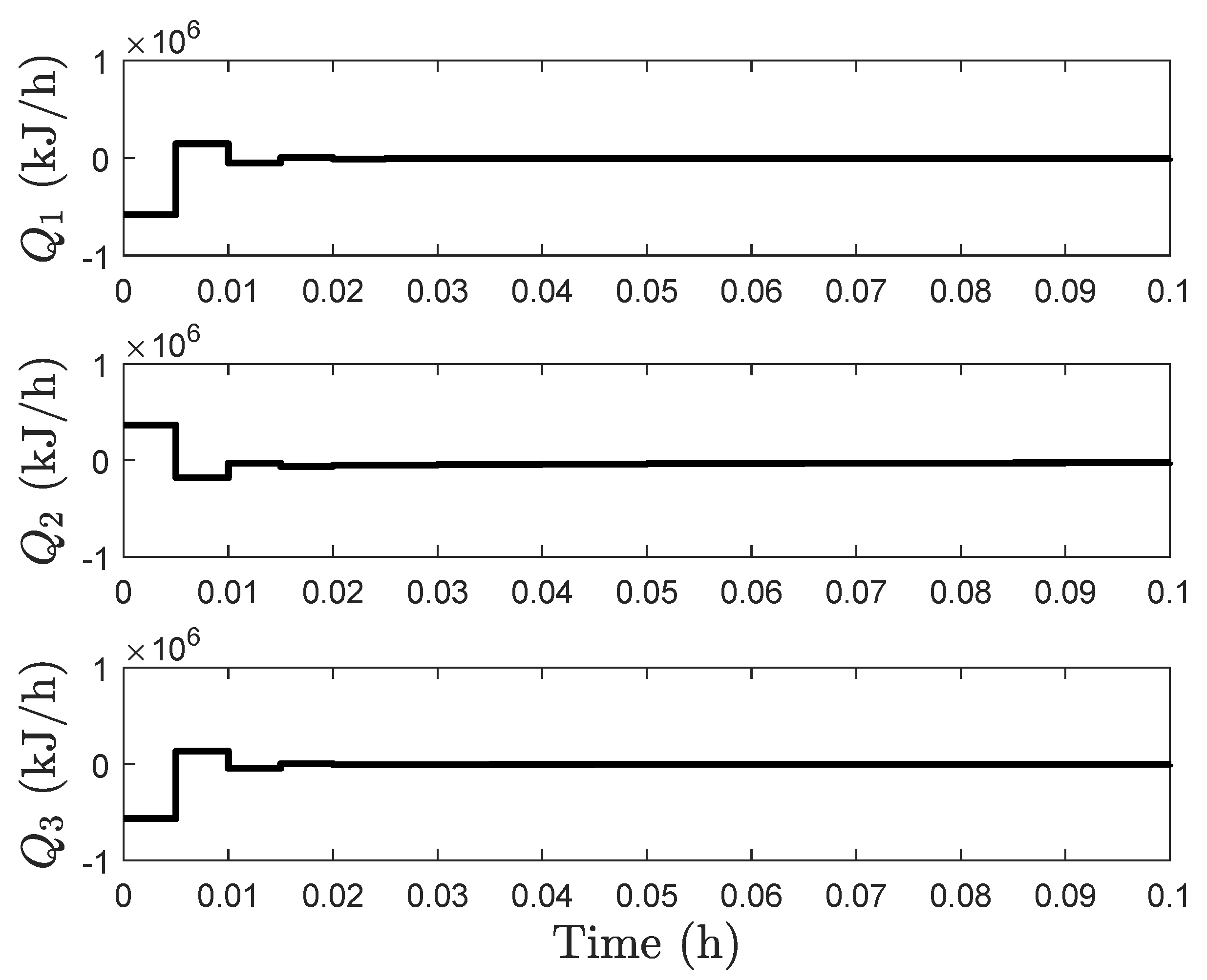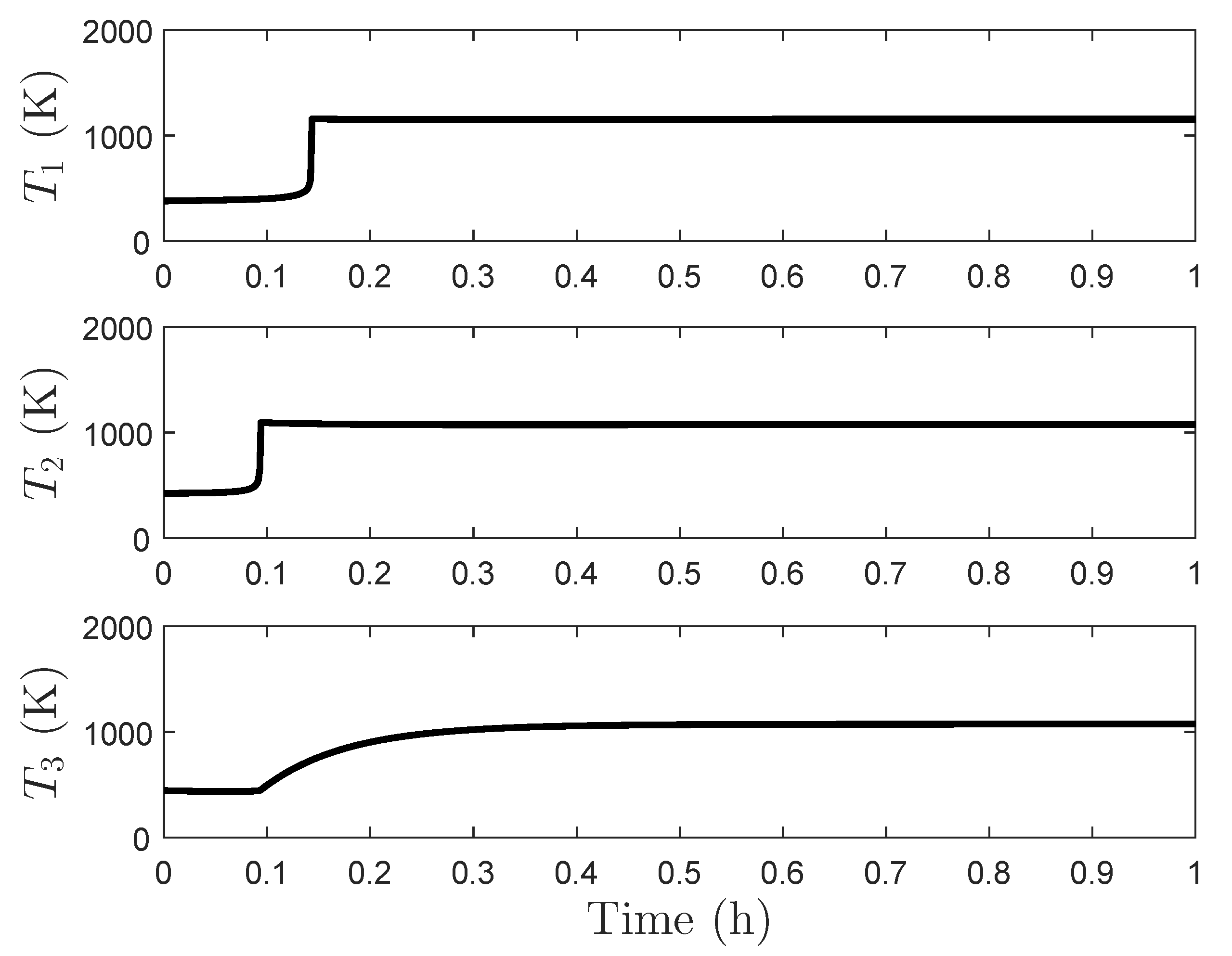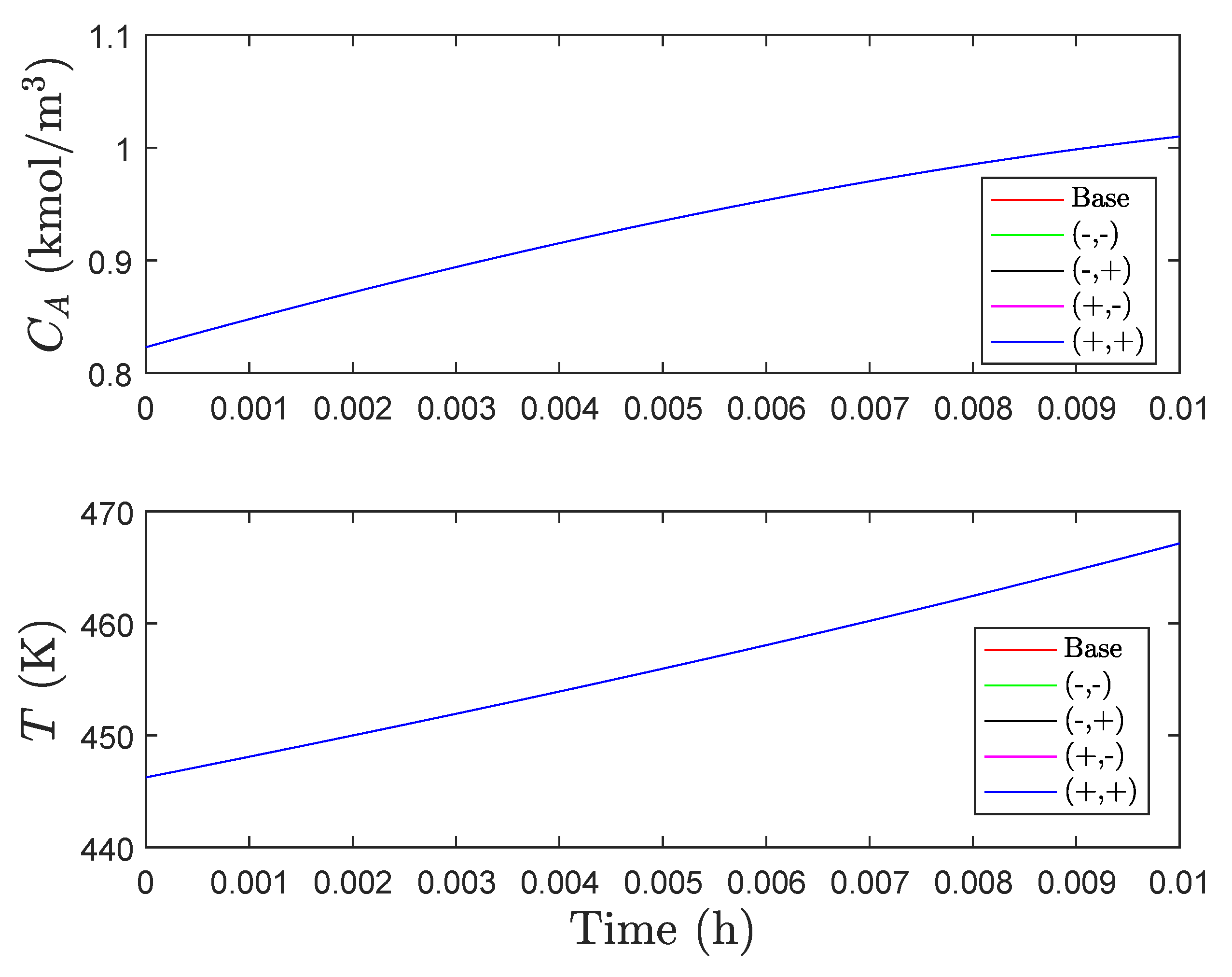The process is operated for one hour with controller parameters of $N=6$ and $\Delta =0.005$ h. MATLAB’s fmincon function was used to solve the MPC optimization problems. Throughout this paper, due to the reasonable controller behavior in all simulations using fmincon, both local minima found by fmincon, as well as possible local minima (without checking whether they were truly local minima) were accepted as solutions to the MPC optimization problems. 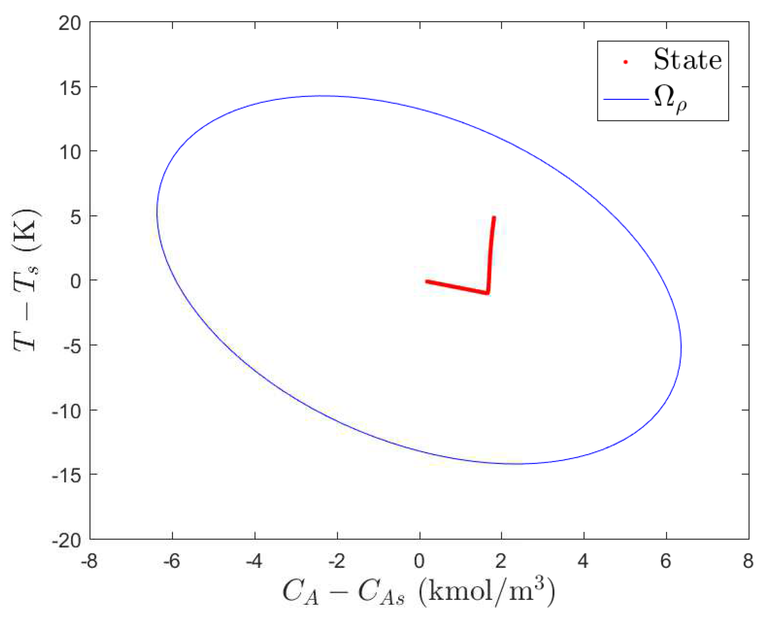Because they will be explored further below, the temperature trajectories in the three vessels and the heat inputs when the process is operated under the MPC designed around the unstable steady-state for the first 0.1 h of operation are shown in Figure 1 and Figure 2. The closed-loop state is observed to be driven to the steady-state value by the controller in the absence of disturbances or plant-model mismatch.

For the design with the parameters in Table 1, we explore the impacts of cyberattacks on the MPC when the process is operated around the unstable steady-state and when it is operated around the stable steady-state. When the MPC is operated around the unstable steady-state (i.e., $q=u$ in Equation (29)) and the process is initialized from $x_I$ = ${\overline{x}}_q$ + $[10$ $0.5$ $-0.001$ $-0.0001$ $-10$ $0.5$ $-0.001$ $-0.0001$ 10 $0.5$ $-0.001$ ${-0.0001]}^T$ but with a false state measurement (denoted by $x_{F1}$) of $x_{F1}={\overline{x}}_u$ provided to the MPC at every sampling time, the state and input trajectories in 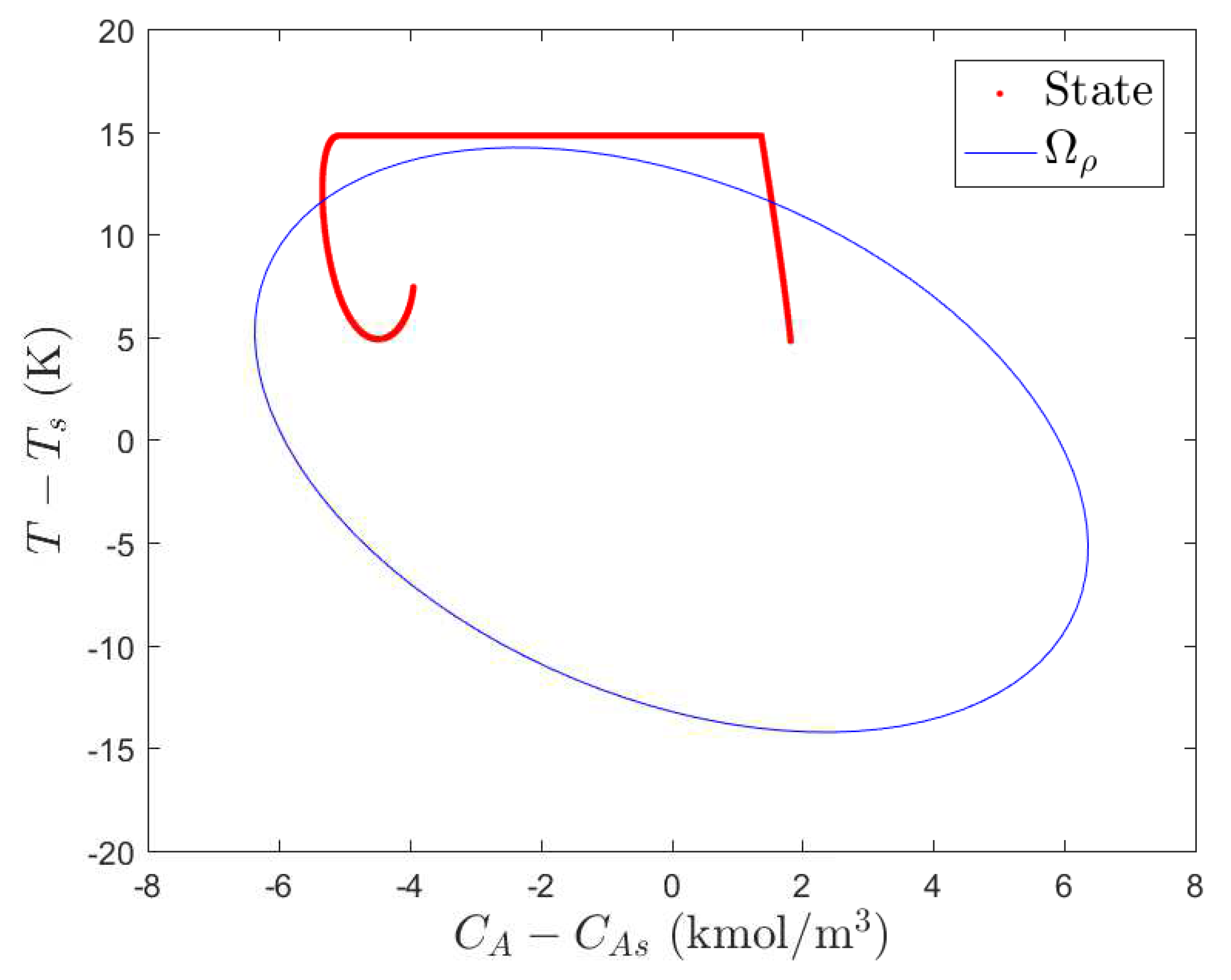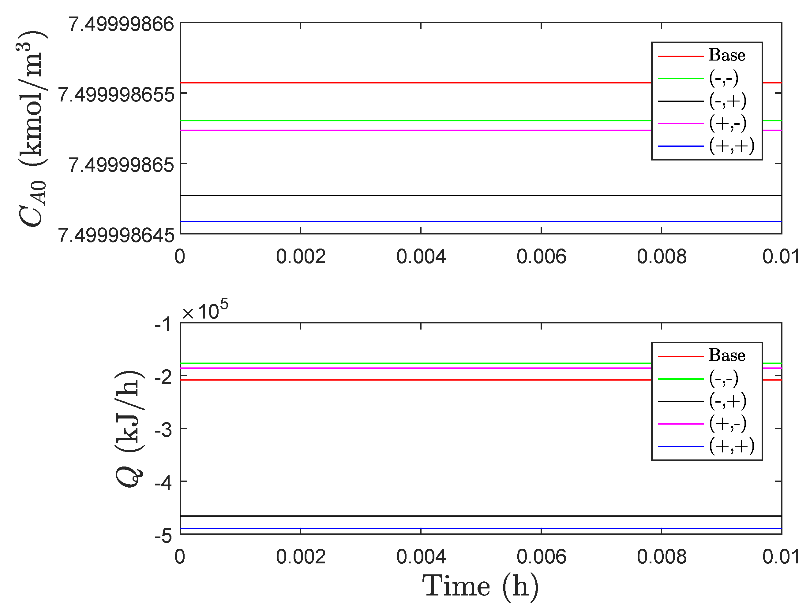Figure 3 and Figure 4 are obtained. This attack takes advantage of nonlinear dynamic behavior (e.g., as shown in Figure 3, the heat rate inputs did not need to be high for the temperatures in the units to become high). In this case, the MPC believes that the state is at the steady-state, and therefore computes the steady-state input, which is not stabilizing for an initial condition slightly off of the steady-state (instead, it causes the closed-loop state to approach a different but stable higher-temperature steady-state). It is noted that this issue may not be able to be readily handled via techniques for accounting for disturbances in MPC (e.g., by estimating the disturbance), as in this case, the controller is not aware of the mismatch between the actual state and the steady-state, and therefore attempts to account for the mismatch between those states as a disturbance would not necessarily be helpful. It also is a relatively easy attack to recognize given the dynamics of unstable systems and the control law considered, despite the multi-unit and interconnected nature of the system. However, fixing of the inputs at the values in Figure 4 is the same effect as would be observed if those actuators were to be fixed at their values via a fault; HAZOP studies should have indicated this and caused the system to be instrumented with, perhaps, a safety valve to prevent the temperatures in the reactor from ever hitting such levels physically. Specifically, because the safety system in that case is actuated based on a problematic process state (pressure) regardless of the path by which that pressure was reached, then whether a cyberattack or a fault caused that condition, the process is protected against it. In contrast, when the process is operated around the stable steady-state (i.e., $q=s$) and the operating steady-state (now ${\overline{x}}_s$) is provided as the false state measurement at every sampling time, this attack strategy drives the closed-loop state to the steady-state ${\overline{x}}_s$ because it causes the MPC to again compute the steady-state input (which for the open-loop stable steady-state is stabilizing from $x_I$).

We now look in greater detail at the role of process design in the success of cyberattacks by analyzing a similar attack on the process described above (i.e., an attack involving a false measurement corresponding to an alternative unstable steady-state ${\overline{x}}_{u,2}$ of a re-designed process being applied to the process initialized at $x_I$ = ${\overline{x}}_{u,2}$ + $[10$ $0.5$ $-0.001$ $-0.0001$ $-10$ $0.5$ $-0.001$ $-0.0001$ 10 $0.5$ $-0.001$ ${-0.0001]}^T$). To re-design the process, it was assumed that though there should be bounds on the states of Vessels 1, 2, and 3, the only states for which it is necessary to maintain the values at specific targets during re-design were the concentration of the product in the product stream ($C_{B3}$) and the concentration of the byproduct in this stream ($C_{C3}$). It was desired to locate a steady-state for this process for which $T_1+T_2+T_3$ was minimized, subject to lower and upper bounds on the vector $v_{dv}$ of decision variables of the re-design ($v_{dv}$ = $[V_1$ $V_2$ $V_3$ $F_{10}$ $T_{10}$ $T_{20}$ $Q_{1,ss}$ $Q_{2,ss}$ $Q_{3,ss}$ $\Delta F_{20,ss}$ $T_{1,ss}$ $C_{A1,ss}$ $C_{B1,ss}$ $C_{C1,ss}$ $T_{2,ss}$ $C_{A2,ss}$ $C_{B2,ss}$ $C_{C2,ss}$ $T_{3,ss}$ $C_{A3,ss}{]}^T$; the lower bound vector was $[0.2$ m${}^3$ 0.2 m${}^3$ 0.2 m${}^3$ 0.2 m${}^3$/h 260 K 260 K $-1\times {10}^6$ kJ/h $-1\times {10}^6$ kJ/h $-1\times {10}^6$ kJ/h −5 m${}^3$/h 260 K 0 kmol/m${}^3$ 0 kmol/m${}^3$ 0 kmol/m${}^3$ 260 K 0 kmol/m${}^3$ 0 kmol/m${}^3$ 0 kmol/m${}^3$ 260 K 0 kmol/m${}^3{]}^T$, and the upper bound vector was $[10$ m${}^3$ 10 m${}^3$ 10 m${}^3$ 10 m${}^3$/h 500 K 500 K $1\times {10}^6$ kJ/h $1\times {10}^6$ kJ/h $1\times {10}^6$ kJ/h 5 m${}^3$/h 500 K 4 kmol/m${}^3$ 3 kmol/m${}^3$ 2 kmol/m${}^3$ 500 K 4 kmol/m${}^3$ 3 kmol/m${}^3$ 2 kmol/m${}^3$ 500 K 4 kmol/m${}^3{]}^T$). MATLAB’s function fmincon was used to find a locally optimal solution to this design problem, subject to the requirement that Equations (14)–(28) be satisfied at the steady-state with $C_{B3}=0.50$ kmol/m${}^3$ and $C_{C3}=0.12$ kmol/m${}^3$ as at the unstable steady-state ${\overline{x}}_u$. The resulting design is $V_1=0.20$ m${}^3$, $V_2=10.00$ m${}^3$, $V_3=5.09$ m${}^3$, $F_{10}=0.21$ m${}^3$/h, $T_{10}=379.98$ K, and $T_{20}=379.99$ K, with the steady-state ${\overline{x}}_{u,s}=[260.00$ K 0.57 kmol/m${}^3$ 0.15 kmol/m${}^3$ 0.05 kmol/m${}^3$ 364.63 K 0.26 kmol/m${}^3$ 0.41 kmol/m${}^3$ 0.10 kmol/m${}^3$ 260.00 K 0.29 kmol/m${}^3$ 0.50 kmol/m${}^3$ 0.12 kmol/m${}^3{]}^T$ corresponding to inputs $Q_{1,ss}=-5809.73$ kJ/h, $Q_{2,ss}=18144.68$ kJ/h, $Q_{3,ss}=-171320.01$ kJ/h, and $\Delta F_{20,ss}=-5.00$ m${}^3$/h. The results from the cyberattack being performed on this process are shown in Figure 5. In contrast to Figure 3 and Figure 4, the maximum temperatures reached in Figure 5 are approximately 919 K for $T_1$, 1003 K for $T_2$, and 895 K for $T_3$, whereas in Figure 3, they are approximately 1156 K for $T_1$, 1093 K for $T_2$, and 1073 K for $T_3$. In the above, only one cyberattack was examined with the design change, but the lower temperatures reached in the time period examined in Figure 5 compared to Figure 3 indicates that for the same design values of $C_{B3}$ and $C_{C3}$, an attack providing the steady-state measurement to an MPC for a process designed around the steady-state in Figure 5 when initiated slightly off that steady-state may be able to be withstood with equipment with a lower design temperature than the process in Figure 3.

4.1.3. Safety-Based Attacks and Control System Cybersecurity: Equipment and Safety System Design

Based on the results of the above sections, when cyberattacks are not seeking to impact conditions which depend on past states and inputs (as might occur with, for example, fatigue) cyberattack resilience of a process design might be analyzed by considering what set of states can be accessed from all initial conditions and under all input trajectories possible, given the system dynamics and any changes in the dynamics as safety systems are activated. This means that, if all allowable initial conditions can be characterized (as, for example, would be theoretically true with LEMPC, where the set of allowable initial conditions could be characterized as those within the set ${\mathrm{\Omega }}_{\rho }$), then simulations can be performed which consider all states which could be reached from these conditions for inputs in the input bounds. For example, from all allowable initial conditions, the state at the next sampling time could be obtained under all possible values of the inputs via simulation (the state and input spaces would need to be discretized to carry this out practically). For each resulting state at the next sampling time that is in the stability region, because the path to that state is not considered important and those states were just tested as initial conditions under all possible inputs to see where the closed-loop state can go at the end of the sampling period, they do not need to be tested again. However, for any that go outside the stability region or access new states not previously tested, further simulations must be done from each of those points until eventually all points that are the final states at the end of each sampling period were already tested as an initial condition for another. This does not account for disturbances, which could also be discretized and the above problem considered for every possible one. Notably, this is no different than the procedure that could be used for faults.

Below, we sketch how this concept for performing such an analysis could be initiated using two continuous stirred tank reactor examples, one which uses a safety system, and one which does not. A goal of the examples in this section is also to clarify the significant similarity between cyberattack-resilient process designs and those which maintain safety under process faults, while also highlighting key differences.

The first system to be explored will revisit an example previously presented in [27], but with a slight change for the purpose of presenting the resilient design mechanism outlined above. This example consists of a continuous stirred tank reactor (CSTR) which is followed by process piping and is considered for converting species A to B, where the piping is rigidly fixed at the CSTR outlet and has a bellows joint with spring constant $k_s$ on the other side. The concentration of reactant $C_A$ and temperature T in the reactor evolve according to the following dynamic model:

$${\dot{C}}_A=\frac{F}{V}(C_{A0}-C_A)-k_0{e}^{-\frac{E}{R_{g}T}}{C}_A^2$$

(30)

$$\dot{T}=\frac{F}{V}(T_0-T)-\frac{\Delta H{k}_0}{{\rho }_L{C}_p}{e}^{-\frac{E}{R_{g}T}}{C}_A^2+\frac{Q}{{\rho }_L{C}_{p}V}$$

(31)

where the inlet reactant concentration $C_{A0}$ and heat rate Q are the manipulated inputs. The parameters F, $k_0$, V, E, $\Delta H$, $R_g$, $C_p$, and ${\rho }_L$ (provided in

Table 2. CSTR process parameters.

Parameter	Value	Units
V	1	m${}^3$
$C_p$	$0.231$	$\frac{\mathrm{kJ}}{\mathrm{kg}\mathrm{K}}$
$T_0$	300	K
$\Delta H$	$-1.15\times {10}^4$	$\frac{\mathrm{kJ}}{\mathrm{kmol}}$
$k_0$	$8.46\times {10}^6$	$\frac{{\mathrm{m}}^3}{\mathrm{h}\mathrm{kmol}}$
F	5	$\frac{{\mathrm{m}}^3}{\mathrm{h}}$
E	$5\times {10}^4$	$\frac{\mathrm{kJ}}{\mathrm{kmol}}$
${\rho }_L$	1000	$\frac{\mathrm{kg}}{{\mathrm{m}}^3}$
$R_g$	$8.314$	$\frac{\mathrm{kJ}}{\mathrm{kmol}\mathrm{K}}$

) correspond to the flow rate through the CSTR, the pre-exponential constant, the CSTR volume, the reaction activation energy, the enthalpy of reaction, the ideal gas constant, the heat capacity of the liquid in the CSTR, and the density of the liquid in the CSTR, respectively.

As in [27], we consider that the goal in characterizing the worst-case conditions under a cyberattack is to select appropriate equipment designs for the CSTR and piping if possible. In particular, we here focus on the value of $k_s$, which could have a significant impact on the ability of the equipment to withstand a cyberattack. To see this, consider that the yield strength of the piping is 270 MPa, and that its thermal expansion coefficient, Young’s Modulus, length, and cross-sectional area are $12.5\times {10}^{-6}$ K${}^{-1}$, 200 GPa, $2.54$ m, and $A=0.002041$ m${}^2$, respectively [36]. The CSTR is controlled by an MPC with the stage cost stage cost:

$$\begin{array}{cc}\hfill L_e=& 100{(C_A-C_{As})}^2+{(T-T_s)}^2+{(C_{A0}-C_{A0s})}^2+{10}^{-10}{(Q-Q_s)}^2\hfill \end{array}$$

(32)

and with the inputs restricted as follows: $0.5\le C_{A0}\le 7.5$ kmol/m${}^3$ and $\left|Q\right|\le 5\times {10}^5$ kJ/h. In [27], this process was examined without additional constraints on the states and inputs. In this section, however, we will extend the work in [27] to present a concept for determining the worst-case conditions which could occur under a cyberattack so that equipment might be designed to withstand it. To analyze the worst-case condition, it is helpful to characterize the set of allowable initial conditions, which is done by using Lyapunov-based stability constraints to bound these conditions. In particular, Lyapunov-based stability constraints are developed around the steady-state $C_{As}=1.22$ kmol/m${}^3$, $T_s=438.2$ K, $C_{A0s}=4$ kmol/m${}^3$, and $Q_s=0$ kJ/h, (i.e., we define $x={\left[x_1{x}_2\right]}^T={[C_A-C_{As}T-T_s]}^T$ and $u={\left[u_1{u}_2\right]}^T={[C_{A0}-C_{A0s}Q-Q_s]}^T$), using $V=x^{T}Px$, with P given as follows:

$$P=\left[\begin{array}{cc}1200& 5\\ 5& 0.1\end{array}\right]$$

(33)

The model of Equations (30) and (31) has the form $\dot{x}=\tilde{f}\left(x\right)+g\left(x\right)u$, where $\tilde{f}$ represents a vector function derived from Equations (30) and (31) that is not multiplied by u, and $g\left(x\right)={\left[g_1{g}_2\right]}^T={[\frac{F}{V}0;0\frac{1}{{\rho }_L{C}_{p}V}]}^T$ represents the vector function which multiplies u in these equations. The Lyapunov-based controller $h_1\left(x\right)$ was designed such that $h_{1,1}\left(x\right)=0$ kmol/m${}^3$ and $h_{1,2}\left(x\right)$ is first computed as follows (Sontag’s Formula [37]):

$$\begin{array}{c}\hfill h_{1,2}\left(x\right)=\left\{\begin{array}{cc}-\frac{L_{\tilde{f}}V+\sqrt{L_{\tilde{f}}{V}^2+L_{{\tilde{g}}_2}{V}^4}}{L_{{\tilde{g}}_2}V},\hfill & \mathrm{if}{L}_{{\tilde{g}}_2}V\ne 0\hfill \\ 0,\hfill & \mathrm{if}{L}_{{\tilde{g}}_2}V=0\hfill \end{array}\right.\end{array}$$

(34)

and then saturated at the input bounds if they are exceeded. $L_{\tilde{f}}V$ and $L_{{\tilde{g}}_2}V$ are Lie derivatives of V with respect to the vector functions $\tilde{f}$ and ${\tilde{g}}_2$, respectively. ${\rho }^{\prime }$ and ${\rho }_e^{\prime }$ were set to 300 and 225, respectively.

It should be noted that in [22], it is demonstrated that when disturbances, the sampling period, and ${\rho }_e$ are sufficiently small, the closed-loop state will not be able to leave ${\mathrm{\Omega }}_{\rho }$ for the process operated under LEMPC. In this example, however, the controller parameters do not meet these requirements, and therefore the simulations do not allow closed-loop stability to be guaranteed. However, because the guarantees could be obtained with modified selection of control design parameters, we use this type of control design to demonstrate how the cyberattack-resilient design methodology would proceed if ${\mathrm{\Omega }}_{\rho }$ was forward invariant such that it represented the allowable set of states without attacks.

The MPC uses a prediction horizon of $N=10$ and a sampling period of $\Delta =0.01$ h, and is solved using MATLAB’s function fmincon. The explicit Euler numerical integration method with an integration step of ${10}^{-4}$ h is used to simulate the process. 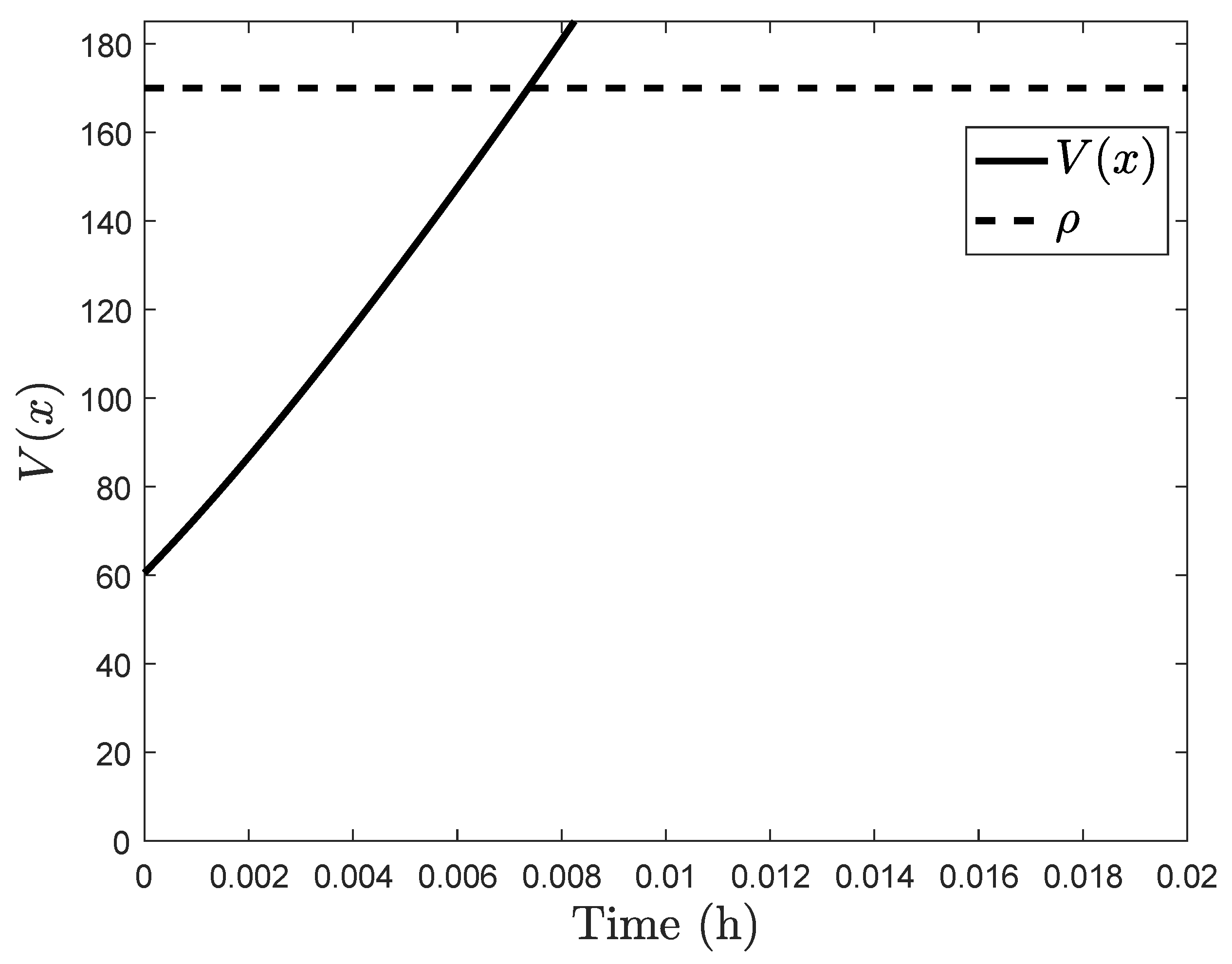The process is initialized off of its steady-state condition $C_A=C_{As}$, $T=T_s$, $C_{A0}=C_{A0s}$, and $Q=Q_s$ from an initial condition at $C_A-C_{As}=-0.4$ kmol/m${}^3$ and $T-T_s=8$ K. When no cyberattack occurs, this controller drives the closed-loop state back to the steady-state. However, when a cyberattack is performed, the temperature of the fluid leaving the CSTR can increase considerably (for example, Figure 6 shows the trajectory when a false state measurement of $C_A\left(t_k\right)=0.8$ kmol/m${}^3$ and $T\left(t_k\right)=430$ K is provided to the MPC at every sampling time for an hour, where the temperature increases by over 400 K above $C_{As}$).

In [27], it was noted that if $k_s$ is unusually stiff (e.g., $k_s=5.5\times {10}^7$ N/m), then yielding could occur for the piping when the temperature is about 278 K greater than its steady-state value. This means that if the piping temperature comes to thermal equilibrium with the fluid leaving the pipe at the end of the time period shown in Figure 6, yielding is possible. In contrast, for a more common (and less stiff) spring constant (e.g., $k_s=4.4\times {10}^5$ N/m [36]), $T-T_s$ would need to be greater than about 39,410 K to cause yielding, which is much greater than the temperature which the piping would be expected to approach according to Figure 6. Therefore, as long as the CSTR itself can withstand the temperature in Figure 6, the piping can be considered to be resilient against the attack on the CSTR’s control system.

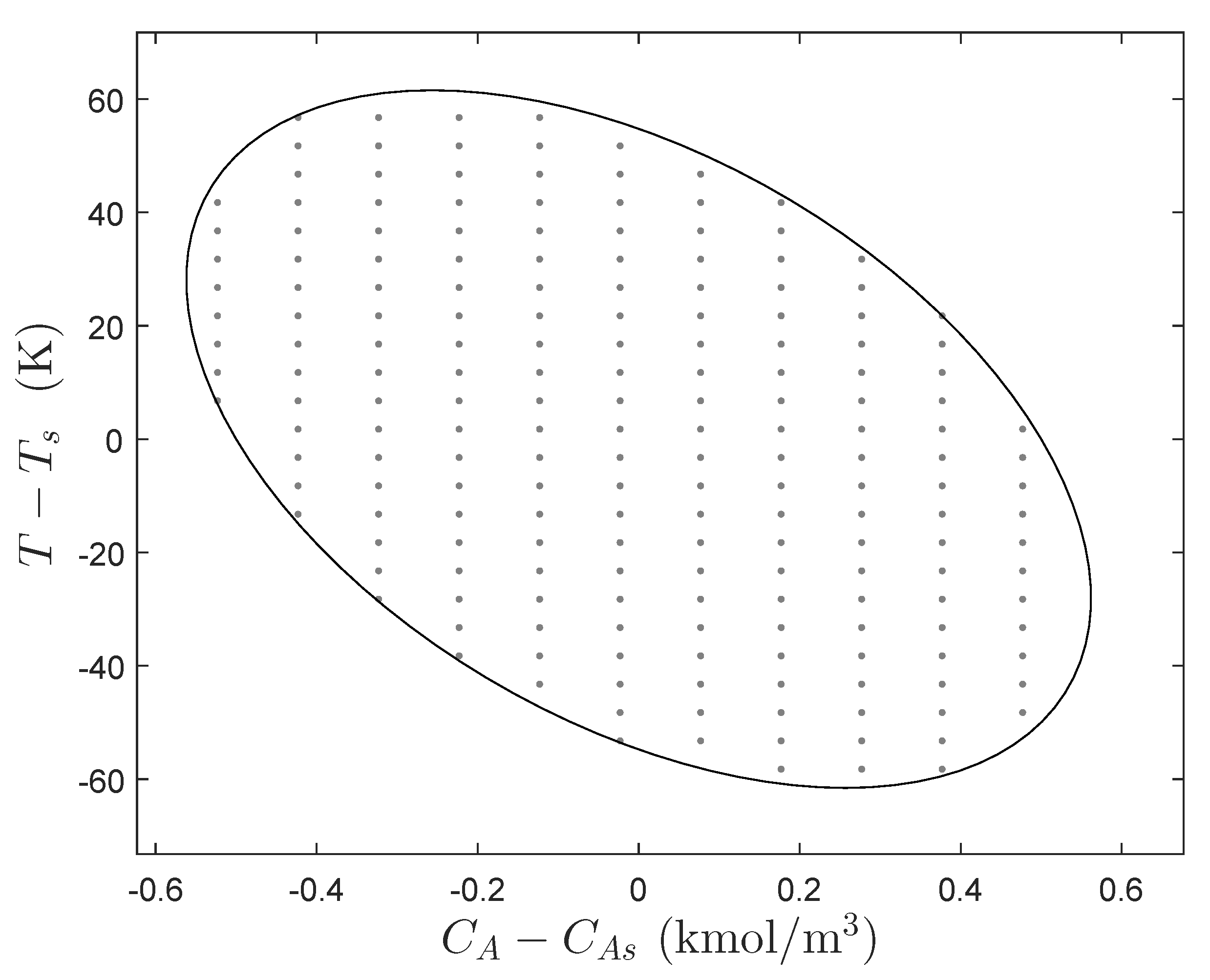
The example above tests one specific initial condition and attack. An exhaustive search technique was suggested above for searching for the worst-case conditions under all attacks. The first step in this search technique was suggested to be characterization of the set of allowable initial conditions, which for LEMPC could be considered to be all the states in the stability region. The state-space can be discretized to identify all of these states for simulation purposes; for the purpose of demonstrating the proposed technique, a relatively coarse discretization (where the points from which the simulation will be carried out are shown in gray in Figure 7) was performed for this example, though a finer one would give more comprehensive results.

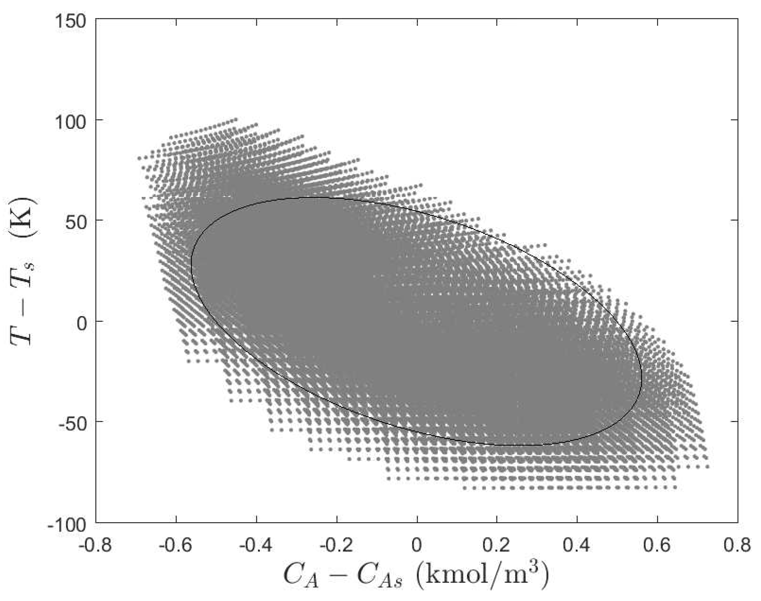
The next step in the proposed procedure is to identify all possible states which could be reached from the set of initial conditions after one sampling period, for any input in the input bounds. For cyberattacks (as well as faults), this represents all possible inputs that could be applied, given any false state measurement or other possible attack. Again using a relatively coarse grid, this can be simulated for this example by finding the final values of the states for $C_{A0}$ between 0.5 and 7.5 kmol/m${}^3$ in increments of 0.5 kmol/m${}^3$, and for Q between $-5\times {10}^5$ and $5\times {10}^5$ kJ/h in units of ${10}^5$ kJ/h. The plots of the resulting initial conditions at the end of a sampling period are shown in Figure 8. The grid was too coarse to capture many of the other final conditions; however, despite only capturing some of the possible final conditions which could occur for various initial conditions in ${\mathrm{\Omega }}_{\rho }$ when inputs in the input bounds are applied for a sampling period, Figure 8 does indicate the concept of the mechanism for checking cyberattack-resilience of a process design. Specifically, after the first sampling period, some of the states under some of the input trajectories are still in ${\mathrm{\Omega }}_{\rho }$; with a finer grid, these points should already have been tested during the first test to see where they would go next under all inputs. Specifically, because the states over the subsequent sampling period do not depend on past values of the states or inputs (i.e., how the state came to be at its initial condition), any final points at the end of the first sampling period (which would serve as initial points for the considerations in the next sampling period) which are the same as those considered at the beginning of the first do not need to be considered in the second sampling period, because the final conditions at the end of the subsequent sampling period were effectively already evaluated by the end of the first sampling period. However, taking all points outside of ${\mathrm{\Omega }}_{\rho }$ at the end of the first sampling period as initial conditions for the second sampling period and analyzing all possible trajectories which could occur within the input bounds after this occurs could be undertaken.

We here highlight that in an actuator fault involving a valve becoming stuck at a given position, the only possible scenarios after the first sampling period as the state evolves from all possible initial conditions under each possible input value are those which have the same input applied as in the prior sampling period. In contrast, in a cyberattack, the input could take any trajectory in any subsequent sampling period. However, if this more conservative approach to evaluating possible worst-case scenarios is used for both cyberattacks and faults, both can be protected against via process design in an equivalent fashion. This may be a very computationally intensive screening method, however, due to the large number of possible scenarios which would need to be evaluated, despite the ability to prune off those where final states from one sampling period correspond to initial states which were already looked at at a prior sampling time in later sampling periods. It should be noted that the equipment must be resilient against even time-varying types of “faulty” behavior, such as fatigue that might be induced by time-varying profiles of the inputs which observers may not be aware of.

In the example above, the discussion focused on ways of checking that an equipment design is fully cyberattack-resilient through an inherently safe design by designing equipment to withstand the worst-case scenarios that could be encountered from any possible state and for any possible inputs. However, this approach may result in a highly conservative and possibly expensive design. An alternative is to add safety systems. For example, consider the methyl isocyanate (MIC) hydrolysis model from [38] in which the hydrolysis reaction is assumed to occur in a CSTR according to the following dynamic equations:

$$\frac{d{C}_A}{dt}=-k_0{e}^{-E/\left(RT\right)}{C}_A+\frac{F}{m}(C_{A0}-C_A)$$

(35)

$$\frac{dT}{dt}=\frac{-\Delta H{k}_0}{C_p}{e}^{-E/\left(RT\right)}{C}_A+\frac{F}{m}(T_0-T)-\frac{U}{m{C}_p}(T-T_j)$$

(36)

where the process parameter values and units corresponding to the mass of the reaction mixture (m), the pre-exponential constant $k_0$, the activation energy E, the ideal gas constant R, the flow rate F through the CSTR, the heat of reaction $\Delta H$, the heat transfer coefficient U, and the inlet fluid temperature $T_0$ are noted in

Table 3. CSTR process parameters for the MIC hydrolysis process [38].

Parameter	Value	Units
$T_0$	293	K
m	$4.1\times {10}^4$	kg
$k_0$	$4.13\times {10}^8$	s${}^{-1}$
$C_p$	3000	J kg${}^{-1}$ K${}^{-1}$
U	$7.1\times {10}^6$	J s${}^{-1}$ K${}^{-1}$
$T_{js}$	293	K
$T_s$	305.1881	K
F	57.5	kg s${}^{-1}$
E	$6.54\times {10}^4$	J mol${}^{-1}$
$\Delta H$	$-8.04\times {10}^4$	J mol${}^{-1}$
R	8.314	J mol${}^{-1}$ K${}^{-1}$
$C_{A0}$	29.35	mol kg${}^{-1}$
$C_{As}$	10.1767	mol kg${}^{-1}$
$A_1$	−20.1597	−
$B_1$	$-1.1878\times {10}^3$	K
$C_1$	$1.3274\times 10$	−
$D_1$	$-2.4414\times {10}^{-2}$	K${}^{-1}$
$E_1$	$1.3907\times {10}^{-5}$	K${}^{-2}$

. The concentration of MIC in the reactor ($C_A$, in mol/kg) and the temperature in the reactor (T, in K) are the states of the process, with the jacket temperature $T_j$ representing the manipulated input. The steady-state values of these variables ($C_{As}$, $T_s$, and $T_{js}$) are also noted in Table 3.

We consider a control and safety system design similar to that from [38]. Specifically, an MPC was designed with the objective function $L_e=3{(C_A-C_{As})}^2+5{(T-T_s)}^2+{(T_j-T_{js})}^2$ and with the Lyapunov-based stability constraint of Equation (12g) using $V=x^{T}Px$ for $P=[20033;3340]$, and the Lyapunov-based controller designed via Sontag’s control law. The bounds on the input are $280\le T_j\le 300$ K, with $\rho =7000$ used in fixing the stability region size as in [38]. The process is simulated under the MPC using an integration step of ${10}^{-3}$ s in an MPC and of ${10}^{-6}$ s for the process, with $N=10$, for 850 s of operation with $\Delta =1$ s. The process state was initialized at $C_a=12$ kmol/m${}^3$ and $T=310$ K. Ipopt [39] was used to perform the simulation with automatic differentiation using ADOL-C [40]. In addition, a safety system was used in which three actions were taken: (1) the state measurements provided to the LEMPC were used to set the value of the manipulated input to its lower bound when $V\left(x\right)>\rho$ (these measurements could be falsified by a cyberattacker who could falsify the state measurements to the LEMPC); (2) a physical mechanism opens a valve when the temperature becomes greater than 320 K in the CSTR and leaves it open for the subsequent time until the temperature drops back below 320 K (physically actuated safety valves typically operate based on pressure rather than temperature exceeding a limit, but in this case, we use temperature for a numerical example that demonstrates the concept of the safety system securing a system against cyberattacks). When the safety valve opens, it is assumed that a mass flow rate of water equal to that of the mass flow rate of fluid leaving through the safety valve exits the CSTR; this flow rate $m_{flow}$ (in kg/m${}^2$ s) is given by:

$$p_1=A_1+\frac{B_1}{T}+C_1{log}_{10}T+D_{1}T+E_1{T}^2$$

(37)

$$p_2=-\frac{B_1}{T^2}+\frac{C_1}{Tln\left(10\right)}+D_1+2E_{1}T$$

(38)

$$m_{flow}=3514.80\sqrt{\frac{T}{C_p}}{10}^{p_1}{p}_1{p}_2$$

(39)

The values of $A_1$, $B_1$, $C_1$, $D_1$, and $E_1$ are given in Table 3, and are set equal to values from [41] for an Antoine-like equation for methyl isocyanate. The form of Equation (39) used in this paper was inspired by a safety valve example from [42], but the safety system design was not rigorously performed for this example. However, the flow rate given by Equation (39) serves to demonstrate the concept of the use of safety systems in arresting the impacts of a cyberattack, as is demonstrated below, and the lack of a rigorous safety system modeling effort does not detract from the overall conclusion that one could simulate the process and its safety system under various possible cyberattacks to understand worst-case scenarios, or whether the safety system allows the design to be resilient against the attacks. The dynamic equations in the presence of the safety system thus become:

$$\frac{d{C}_A}{dt}=-k_0{e}^{-E/\left(RT\right)}{C}_A+\frac{F}{m}(C_{A0}-C_A)-\frac{m_{flow}{A}_{SV}{C}_A}{m}$$

(40)

$$\frac{dT}{dt}=\frac{-\Delta H{k}_0}{C_p}{e}^{-E/\left(RT\right)}{C}_A+\frac{F}{m}(T_0-T)-\frac{U}{m{C}_p}(T-T_j)+\frac{m_{flow}{A}_{SV}}{m}(T_{cooling}-T)$$

(41)

where $A_{SV}=0.4$ m${}^3$ represents the safety valve area (selected for the purpose of allowing the safety system to combat a cyberattack as will be demonstrated below) and $T_{cooling}=280$ K is the temperature of the cooling water stream that is injected into the reactor as part of the safety system. The heat capacity of all streams, including the pure water stream, is taken to be $C_p$ for simplicity; despite a large number of modeling assumptions that are not true physically in this example, it is effective at showing the concept of the safety system preventing the cyberattack success, as discussed below.

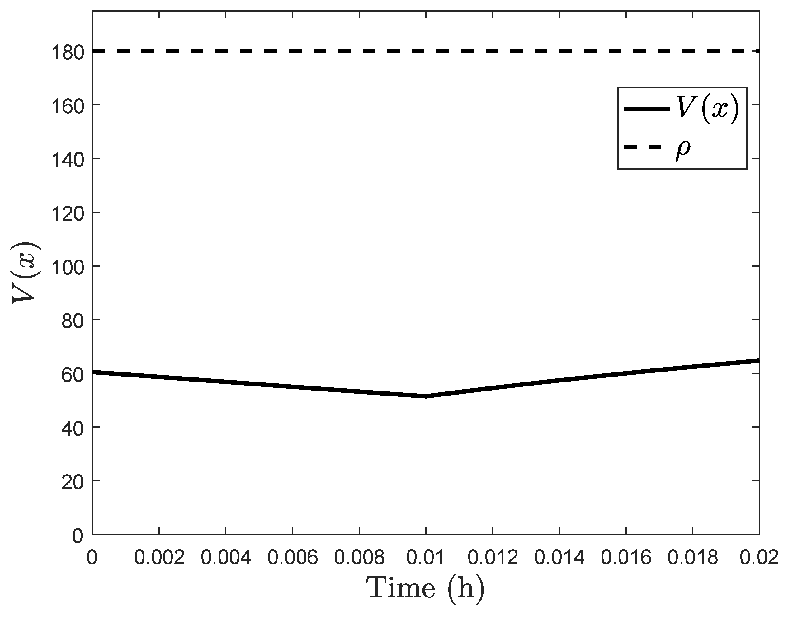
Specifically, Figure 9 shows the state-space trajectory when the system is controlled by the MPC described above and started from an initial condition off the steady-state (i.e., $C_A=12$ kmol/m${}^3$, $T=310$ K), in the absence of a cyberattack (i.e., accurate state measurements are provided to the MPC at every sampling time). In the presence of an attack involving the false state measurement $C_A=11$ kmol/m${}^3$, $T=300$ K provided to the MPC at every sampling time, even though the closed-loop state exits the region ${\mathrm{\Omega }}_{\rho }$ as in Figure 10 (which shows 300 s of operation), the safety system activates and drives it back into the stability region. If this type of test were performed for all possible initial conditions and inputs in the input bounds (which are all the possible ones which a cyberattacker providing false state measurements or other attacks would be able to cause) in the presence of the safety system to ensure that the safety system is able to prevent any attack from causing an issue, the system including the safety system could be concluded to be cyberattack-resilient as long as the safety system does not fail (even if it would not have been resilient without the safety system activating).

The outcome of the above analysis is that many processes today may find that they already have cyberattack-resilient designs if the initial designs were made fault-tolerant; however, the results above suggest a method by which organizations may evaluate whether this is true for their own designs and better understand the assumptions under which original designs were developed may differ from the assumptions necessary when considering cyberattack-resilience.

4.1.4. Understanding Safety-Based Attacks and Control System Cybersecurity in Light of Industrial Safety Practice

The two above examples take an inherent safety perspective on cyberattacks. In general, one would expect that good process design practice within a traditional safety framework (e.g., HAZOP) should eliminate many safety issues that could arise from cyberattacks on the control systems. In particular, a state-based approach to safety [33] in which all hazardous states are identified and ways of activating the safety systems when such states are reached would be expected to alleviate any potential consequences of a cyberattack. This would hold then regardless of the path by which the attacker manages to create the problem (e.g., whether there exists some stealthy route by which to set up a problematic state within a unit). The question that remains open from a safety perspective is then perhaps the question of whether all conditions in state-space that could correspond to an unsafe operating condition and could be impacted by a cyberattack are identified and incorporated within the safety system today. Essentially, the question is, what have the designers allowed the system to do? For example, consider level control of a tank. If the tank is designed so that even at the maximum flow rate possible out of the actuator, the tank cannot overflow, then even if an attacker gains control over the level control loop and in a worst case takes the flow rate to its maximum value, the tank cannot overflow. Even in the case of the Stuxnet attacks, the system failed because the centrifuges were able to spin at rates that would destroy them. Had an upper bound been specified on their rate of rotation physically, they would not have been able to be broken by an attack. However, perhaps the nuance with cyberattacks is what types of dynamic operating conditions might be set up by an attacker with control over the time behavior of the actuators, and not just, as would be more expected in the case of an actuator fault, their position. For such a case, potentially it is not only the states that are important, but how they accumulate over time. For example, equipment life is predicted based on experience with a typical operating policy. If cyberattacks could alter that typical operating policy, the question is whether they could potentially break process equipment at a different time than expected. This may be able to be handled with sufficient safety factors in design and routine maintenance/maintenance checks. The above suggests that considering cyberattacks during a HAZOP may be beneficial at locating new worst-case scenarios to instrument systems against, and also for incorporating process dynamic effects in safety analysis.

5. Profit/Production-Based Attacks and Control System Cybersecurity

Though safety concerns for cyberattacks represent the most crucial issues to address from a cybersecurity standpoint, as addressed above, attacks intending to impact economics also pose a threat, and methods for preventing these could also be applied to preventing safety incidents. We consider that one way that companies may be able to move toward addressing this issue is by using a control design that ensures that the closed-loop state cannot leave a bounded region of operation within a sampling period, under the assumption that a detection mechanism can be developed that can detect the attack within a sampling period. This section assumes the existence of such a detection mechanism, and develops the conditions under which the closed-loop state would be maintained in a bounded region for a sampling period if an attack occurs. Future work can seek to identify attack detection mechanisms and integrate them with the proposed approach to analyze the potential of this technique for reducing damage from profitability-focused cyberattacks. The premise is that if the closed-loop state can be maintained within a bounded region of state-space, the worst-case profit loss in that region could be assessed a priori through closed-loop simulations of the state, from any initial condition in that region, under any input in the input bounds and with all possible disturbance realizations, which could reveal both the best-case and worst-case profits over the subsequent sampling period. The difference between these then serves as an upper bound on the potential profit loss over that sampling period before an attack is detected. If the attack can be detected within a sampling period, then mitigating actions (including stopping the use of the false state measurements in determining control actions) can be performed to prevent significant profit/production loss. If the worst-case profits are not acceptable, the sampling period length and the size of the stability region could be tuned to attempt to modify the worst-case condition.

5.1. Cyberattack-Resilient Lyapunov-based Economic Model Predictive Control for Profit/Production-Based Cyberattacks: Formulation

In this section, we develop a controller formulation that, as suggested in the above section, ensures that the closed-loop state remains within a bounded operating region ${\mathrm{\Omega }}_{{\rho }^{\prime }}\subset {\mathrm{\Omega }}_{\rho }$, both in the absence of a cyberattack, and for at least one sampling period in the presence of an attack involving false state measurements being provided to the sensors as long as the false state measurement deviation from the actual measurement is within a bound to be characterized below. We assume that the false state measurements which must be considered are within ${\mathrm{\Omega }}_{{\rho }^{\prime }}$ (or else the attack would be detected by the closed-loop state deviating from its theoretically guaranteed behavior, which is that it must remain within ${\mathrm{\Omega }}_{{\rho }^{\prime }}$ in the absence of an attack). The method presented below is not restricted from a control design perspective to any number of sensors being attacked; however, [43] characterizes observability conditions for detecting attacks on linear systems, and the assumed detection algorithm may thus require that no more than a certain number of sensors be attacked to function correctly; characterizing this, however, is outside the scope of this work. The proposed LEMPC formulation is as follows:

$$\begin{array}{}\mathrm{(42a)}& \hfill \underset{u\left(t\right)\in S(\Delta )}{min}& {\int }_{t_k}^{t_{k+N}}{L}_e(\tilde{x}\left(\tau \right),u\left(\tau \right))d\tau \hfill \mathrm{(42b)}& \hfill \mathrm{s}.\mathrm{t}.& \dot{\tilde{x}}\left(t\right)=f(\tilde{x}\left(t\right),u\left(t\right),0)\hfill \mathrm{(42c)}& & \tilde{x}\left(t_k\right)=x\left(t_k\right)\hfill \mathrm{(42d)}& & \tilde{x}\left(t\right)\in X,\forall t\in [t_k,t_{k+N})\hfill \mathrm{(42e)}& & u\left(t\right)\in U,\forall t\in [t_k,t_{k+N})\hfill \mathrm{(42f)}& & |u_i\left(t_k\right)-h_{1,i}\left(\tilde{x}\left(t_k\right)\right)|\le {ϵ}_r,i=1,\dots ,m\hfill & & |u_i\left(t_j\right)-h_{1,i}\left(\tilde{x}\left(t_j\right)\right)|\le {ϵ}_r,i=1,\dots ,m,\hfill \mathrm{(42g)}& & j=k+1,\dots ,k+N-1\hfill & & V\left(\tilde{x}\left(t\right)\right)\le {\rho }_e^{\prime },\forall t\in [t_k,t_{k+N}),\hfill \mathrm{(42h)}& & \mathrm{if}x\left(t_k\right)\in {\mathrm{\Omega }}_{{\rho }_e^{\prime }}\hfill & & \frac{\partial V\left(x\left(t_k\right)\right)}{\partial x}f(x\left(t_k\right),u\left(t_k\right),0)\hfill & & \le \frac{\partial V\left(x\left(t_k\right)\right)}{\partial x}f(x\left(t_k\right),h_1\left(x\left(t_k\right)\right),0)\hfill \mathrm{(42i)}& & \mathrm{if}x\left(t_k\right)\in {\mathrm{\Omega }}_{{\rho }^{\prime }}/{\mathrm{\Omega }}_{{\rho }_e^{\prime }}\hfill \end{array}$$

This formulation is similar to that in Equation (11), except that it replaces ${\rho }_e$ and $\rho$ with ${\rho }_e^{\prime }$ and ${\rho }^{\prime }$, respectively, where ${\rho }_e^{\prime }<{\rho }_e$ and ${\rho }^{\prime }<\rho$, with ${\mathrm{\Omega }}_{{\rho }_e^{\prime }}\subset {\mathrm{\Omega }}_{{\rho }^{\prime }}$, and includes the input rate of change constraints from [26]. This is done to ensure that even if the closed-loop state leaves a set ${\mathrm{\Omega }}_{{\rho }^{\prime }}$ within a sampling period under a cyberattack, it is still within a larger set ${\mathrm{\Omega }}_{\rho }$ within which the Lyapunov-based controller $h_1\left(x\right)$, if subsequently provided with accurate state measurements, is able to drive the closed-loop state back into ${\mathrm{\Omega }}_{{\rho }^{\prime }}$.

5.2. Cyberattack-Resilient Lyapunov-based Economic Model Predictive Control for Profit/Production-Based Cyberattacks: Implementation Strategy

In this section, we present a possible implementation strategy for cyberattack-resilient control that relies on sufficient conservatism in ${\mathrm{\Omega }}_{{\rho }^{\prime }}$ compared to ${\mathrm{\Omega }}_{\rho }$ based on how large a sampling period $\Delta$ is. Attacks are assumed to be flagged at $t_k$ if $x\left(t_k\right)$ is more than $|{\delta }^{\prime }|$ off of a predicted value $x_p\left(t_k\right)$ for the state (predicted from state predictions using the dynamic model of Equation (42b)); specifically, if $|x\left(t_k\right)-x_p\left(t_k\right)|>|{\delta }^{\prime }|$, then an attack is flagged. As will be shown in the stability and feasibility analysis for this proposed strategy, the value of ${\delta }^{\prime }$ selected will impact the conservativeness of ${\mathrm{\Omega }}_{{\rho }^{\prime }}$ compared to ${\mathrm{\Omega }}_{\rho }$. However, the proposed strategy does not make provision for selecting a value of ${\delta }^{\prime }$ that will avoid false positives in terms of cyberattack detection.

The proposed implementation strategy is as follows: At $t_k$, the state measurement $x\left(t_k\right)$ is obtained. If $|x\left(t_k\right)-x_p\left(t_k\right)|>|{\delta }^{\prime }|$, consider that a cyberattack is occurring and use a backup strategy (e.g., redundant sensors) to obtain correct state measurements for use in controlling the process under the LEMPC of Equation (42). If $|x\left(t_k\right)-x_p\left(t_k\right)|\le |{\delta }^{\prime }|$, control the process using the LEMPC of Equation (42) for the next sampling period. Assuming the availability of a cyberattack detection technique that can locate a cyberattack within the next time period $\Delta$ using measurements of the process state at more frequent intervals between $t_k$ and $t_{k+1}$ (where at these more frequent intervals, the LEMPC is not re-solved), the closed-loop state will not leave ${\mathrm{\Omega }}_{\rho }$ over the next sampling period even if $|x\left(t_k\right)-x_p\left(t_k\right)|\le |{\delta }^{\prime }|$ but an attack occurred.

5.3. Cyberattack-Resilient Lyapunov-based Economic Model Predictive Control for Profit/Production-Based Cyberattacks: Stability and Feasibility Analysis

In this section, we demonstrate that inputs computed by the LEMPC of Equation (42) are guaranteed to maintain the closed-loop state of the process of Equation (1) within ${\mathrm{\Omega }}_{\rho }$ for a sampling period under sufficient conditions if a falsified state measurement satisfying $|x\left(t_k\right)-x_p\left(t_k\right)|\le |{\delta }^{\prime }|$ is provided in Equation (42c). We first note that when accurate state measurements are provided, closed-loop stability of the system of Equation (1) follows from the results in [22,26]. Therefore, this section develops the theory for the closed-loop state evolution under a cyberattack for this LEMPC. Because we look at the evolution of the state over a single sampling period after a cyberattack occurs, without loss of generality, we consider that the time at the start of that sampling period is $t_0=0$.

We note that the LEMPC of Equation (42) computes different control actions depending on the value of $x\left(t_0\right)$. We are interested in bounding how much the actual process state trajectory when the falsified state measurement is provided to the LEMPC deviates from the trajectory when the true state measurement is provided after a sampling period, and in particular under what conditions bounding the predicted state trajectory under the optimal input resulting from the falsified state measurement would correspond to bounding the actual state trajectory under the same input within a pre-specified region. In summary, the cyberattack situation considered in this section is as follows:

Definition 4.

Consider the state trajectories from $t\in [t_0,t_1)$ that are the solutions of the systems

$${\dot{x}}_a=f(x_a\left(t\right),\overline{u},w\left(t\right))$$

(43)

and

$${\dot{x}}_b=f(x_b\left(t\right),\widehat{u},w\left(t\right))$$

(44)

where $x_a\left(t_0\right)=x_b\left(t_0\right)=x_0$, where $\overline{u}$ is the optimal input for $t\in [t_0,t_1)$ computed from the LEMPC of Equation (42) with the state measurement $x_0$, while $\widehat{u}$ is the optimal input for $t\in [t_0,t_1)$ computed from the LEMPC of Equation (42) with the state measurement $x_0+\delta$, where $x_0+\delta$ is a falsified state measurement. The trajectory $x_a\left(t\right)$, $t\in [t_0,t_1)$, represents the behavior of the process in the absence of a cyberattack over the sampling period from $t_0$ to $t_1$, whereas the trajectory $x_b\left(t\right)$, $t\in [t_0,t_1)$, represents the behavior of the process over the sampling period from $t_0$ to $t_1$ when a cyberattack consisting of a sufficiently small state measurement falsification (i.e., $\left|\delta \right|$ is sufficiently small) is performed at $t_0$.

The relationship between $\delta$ and ${\delta }^{\prime }$ will be clarified below. Because changes in the initial condition in Equation (42) change the constraint set of the LEMPC, it would be expected that the input that the LEMPC will compute may vary with changes in this initial condition. Therefore, it is expected that $x_a\left(t_1\right)\ne x_b\left(t_1\right)$. However, if $\Delta$ is small enough, it would be expected that these are not too different due to continuous dependence on initial conditions [44].

The motivation for using the input rate of change constraints in Equation (42) is that analyzing the differences in the state trajectories $x_a$ and $x_b$ in Definition 4 requires an understanding of the magnitude of the difference between $\overline{u}$ and $\widehat{u}$. The input rate of change constraints allow the differences between the inputs computed when the different initial conditions are provided to the EMPC to be bounded in a manner that depends on the constraint form. Specifically, we assume as in [12] that the attacker may avoid detection by providing a falsified state measurement trajectory where the state measurements at every sampling time are within ${\mathrm{\Omega }}_{{\rho }^{\prime }}$; because feasibility of the LEMPC of Equation (42) was proven in [26] to hold when the measurement in Equation (42c) is in ${\mathrm{\Omega }}_{{\rho }^{\prime }}$, feasibility of the LEMPC at $t_0$ is ensured whether or not there is an attack at that sampling time. Furthermore, due to the fact that the optimal solution will be feasible, the optimal values of the input vectors $\overline{u}\left(t_0\right)$ and $\widehat{u}\left(t_0\right)$ in Definition 4, for which the components will be denoted by ${\overline{u}}_i\left(t_0\right)$ and ${\widehat{u}}_{1,i}\left(t_0\right)$, $i=1,\dots ,m$, respectively, satisfy:

$$|{\overline{u}}_i\left(t_0\right)-h_{1,i}\left({\tilde{x}}_a\left(t_0\right)\right)|\le {ϵ}_r$$

(45)

$$|{\widehat{u}}_i\left(t_0\right)-h_i\left({\tilde{x}}_b\left(t_0\right)\right)|\le {ϵ}_r$$

(46)

The following proposition bounds the difference between $x_a$ and $x_b$ in Definition 4 by taking advantage of the input rate of change constraints in Equations (45) and (46).

Proposition 1.

Consider the systems in Definition 4 operated under the LEMPC of Equation (42) designed based on a controller $h_1(·)$ satisfying Equations (2)–(6). The following bound holds:

$$|x_a\left(t\right)-x_b\left(t\right)|\le f_u\left(t\right)$$

(47)

for $t\in [0,t_1)$, where

$$f_u\left(\tau \right):=\frac{L_u(2{ϵ}_r+L_h\left|\delta \right|)\sqrt{m}}{L_x}(e^{L_x\tau }-1)$$

(48)

Proof. 

The proof consists of two parts. In the first part, we demonstrate that due to Equations (45)–(46), $|\overline{u}-\widehat{u}|$ is bounded. In the second part, we use this bound to derive Equation (48).

Part 1. The difference in the inputs $\overline{u}$ and $\widehat{u}$ which would be applied to the process if the accurate measurement ${\tilde{x}}_a\left(t_0\right)=x_0$ is provided to the LEMPC of Equation (42) at $t_0$ compared to if the false measurement ${\tilde{x}}_b\left(t_0\right)=x_0+\delta$ is provided can be bounded due to the use of the input rate of change constraints and Equation (6) as follows:

$$\begin{array}{cc}\hfill & |{\overline{u}}_i\left(t_0\right)-{\widehat{u}}_i\left(t_0\right)|\hfill \\ \hfill & =|{\overline{u}}_i\left(t_0\right)+h_{1,i}\left({\tilde{x}}_a\left(t_0\right)\right)-h_{1,i}\left({\tilde{x}}_a\left(t_0\right)\right)+h_{1,i}\left({\tilde{x}}_b\left(t_0\right)\right)\hfill \\ \hfill & -h_{1,i}\left({\tilde{x}}_b\left(t_0\right)\right)-{\widehat{u}}_i\left(t_0\right)|\hfill \\ \hfill & \le |{\overline{u}}_i\left(t_0\right)-h_{1,i}\left({\tilde{x}}_a\left(t_0\right)\right)|+|h_{1,i}\left({\tilde{x}}_a\left(t_0\right)\right)-h_{1,i}\left({\tilde{x}}_b\left(t_0\right)\right)|\hfill \\ \hfill & +|{\widehat{u}}_i\left(t_0\right)-h_{1,i}\left({\tilde{x}}_b\left(t_0\right)\right)|\hfill \\ \hfill & \le 2{ϵ}_r+L_h|{\tilde{x}}_a\left(t_0\right)-{\tilde{x}}_b\left(t_0\right)|\hfill \\ \hfill & \le 2{ϵ}_r+L_h\left|\delta \right|\hfill \end{array}$$

(49)

for all $i=1,\dots ,m$, and ${\tilde{x}}_a\left(t_0\right),{\tilde{x}}_b\left(t_0\right)\in {\mathrm{\Omega }}_{{\rho }^{\prime }}$. Thus, the differences in the components of the inputs $\overline{u}$ and $\widehat{u}$ that would be computed at $t_0$ with and without the cyberattack are bounded in Equation (49) by a bound that depends on how deviant the false state measurement was from the actual state measurement (i.e., $\delta$).

Part 2. Consider now the actual state trajectories $x_a$ and $x_b$ given by Equations (43)–(44) under the two different inputs $\overline{u}$ and $\widehat{u}$ throughout the sampling period from $t_0$ to $t_1$. In this case:

$$x_a\left(t\right)=x_a\left(t_0\right)+{\int }_{t_0}^{t}f(x_a\left(s\right),\overline{u},w)ds$$

(50)

$$x_b\left(t\right)=x_b\left(t_0\right)+{\int }_{t_0}^{t}f(x_b\left(s\right),\widehat{u},w)ds$$

(51)

Subtracting Equation (51) from Equation (50) and taking the absolute value of both sides gives:

$$\begin{array}{cc}\hfill & |x_a\left(t\right)-x_b\left(t\right)|\hfill \\ \hfill & \le {\int }_0^t\left[|f(x_a\left(s\right),\overline{u},w\left(s\right))-f(x_b\left(s\right),\widehat{u},w\left(s\right))|\right]ds\hfill \\ \hfill & ={\int }_0^t\left[|f(x_a\left(s\right),\overline{u},w\left(s\right))-f(x_a\left(s\right),\widehat{u}\left(s\right),w\left(s\right))\right.\hfill \\ \hfill & \left.+f(x_a\left(s\right),\widehat{u}\left(s\right),w\left(s\right))-f(x_b\left(s\right),\widehat{u},w\left(s\right))|\right]ds\hfill \\ \hfill & \le {\int }_0^t\left[|f(x_a\left(s\right),\overline{u},w\left(s\right))-f(x_a\left(s\right),\widehat{u}\left(s\right),w\left(s\right))|\right.\hfill \\ \hfill & \left.+|f(x_a\left(s\right),\widehat{u}\left(s\right),w\left(s\right))-f(x_b\left(s\right),\widehat{u},w\left(s\right))|\right]ds\hfill \end{array}$$

(52)

for all $t\in [0,t_1)$. Using Equations (8) and (9), the following bound is achieved:

$$\begin{array}{cc}\hfill & |x_a\left(t\right)-x_b\left(t\right)|\le {\int }_0^t\left[L_u|\overline{u}\left(0\right)-\widehat{u}\left(0\right)|+L_x|x_a\left(s\right)-x_b\left(s\right)|\right]ds\hfill \\ \hfill & \le L_u|\overline{u}\left(0\right)-\widehat{u}\left(0\right)|(t-0)+L_x{\int }_0^t|x_a\left(s\right)-x_b\left(s\right)|ds\hfill \\ \hfill & \le L_u(2{ϵ}_r+L_h\left|\delta \right|)\sqrt{m}t+L_x{\int }_0^t|x_a\left(s\right)-x_b\left(s\right)|ds\hfill \end{array}$$

(53)

for all $t\in [0,t_1)$, where the last inequality follows from Equation (49). Finally, using the Gronwall-Bellman inequality [44], it is obtained that:

$$|x_a\left(t\right)-x_b\left(t\right)|\le \frac{L_u(2{ϵ}_r+L_h\left|\delta \right|)\sqrt{m}}{L_x}(e^{L_{x}t}-1)$$

(54)

for $t\in [0,t_1)$. □

We now present two propositions, the first of which bounds the difference between the trajectories of the actual and nominal systems of Equation (1) when initialized from the same state, and the second of which uses the following proposition to relate ${\delta }^{\prime }$ and $\delta$.

Proposition 2.

[22,45] Consider the systems

$${\dot{x}}_y\left(t\right)=f(x_y\left(t\right),\overline{u}\left(t\right),w\left(t\right))$$

(55)

$${\dot{x}}_z\left(t\right)=f(x_z\left(t\right),\overline{u}\left(t\right),0)$$

(56)

with initial states $x_y\left(t_0\right)=x_z\left(t_0\right)\in {\mathrm{\Omega }}_{\rho }$. There exists a $\mathcal{K}$ function $f_W(·)$ such that

$$|x_y\left(t\right)-x_z\left(t\right)|\le f_W(t-t_0)$$

(57)

for all $x_y\left(t\right),x_z\left(t\right)\in {\mathrm{\Omega }}_{\rho }$ and all $w\left(t\right)\in W$ with:

$$f_W\left(\tau \right)=\frac{L_w\theta }{L_x}(e^{L_x\tau }-1)$$

(58)

Proposition 3.

Consider that the following holds:

$$|{\tilde{x}}_b\left(t_{k+1}\right)-x_p\left(t_{k+1}\right)|\le |{\delta }^{\prime }|$$

(59)

where $x_p\left(t_{k+1}\right)$ is the solution of the nominal system of Equation (1) initialized from the last (accurate) state measurement at $t_k$, then if

$$f_W(\Delta )+|{\delta }^{\prime }|\le |\delta |$$

(60)

the following holds:

$$|{\tilde{x}}_a\left(t_{k+1}\right)-{\tilde{x}}_b\left(t_{k+1}\right)|\le |\delta |$$

(61)

Proof. 

From the triangle inequality, Equation (57), and Equations (59) and (60):

$$\begin{array}{cc}\hfill & |{\tilde{x}}_a\left(t_{k+1}\right)-{\tilde{x}}_b\left(t_{k+1}\right)|=|{\tilde{x}}_a\left(t_{k+1}\right)-x_p\left(t_{k+1}\right)+x_p\left(t_{k+1}\right)-{\tilde{x}}_b\left(t_{k+1}\right)|\hfill \\ \hfill & \le |{\tilde{x}}_a\left(t_{k+1}\right)-x_p\left(t_{k+1}\right)|+|x_p\left(t_{k+1}\right)-{\tilde{x}}_b\left(t_{k+1}\right)|\hfill \\ \hfill & \le f_W(\Delta )+|{\delta }^{\prime }|\le |\delta |\hfill \end{array}$$

(62)

The use of Equation (57) in the above statement assumes that the measurement at $t_k$ was accurate (i.e., $x_p\left(t_k\right)={\tilde{x}}_a\left(t_k\right)$). □

The above proposition indicates that the proposed implementation strategy (i.e., if $|x\left(t_k\right)-x_p\left(t_k\right)|>|{\delta }^{\prime }|$, a warning is presented to operators) can be used to guarantee that the actual state and the state measurement are within a certain bound at the first sampling period when the state measurement is falsified and that has not yet been detected. This will be used in proving that the closed-loop state remains within ${\mathrm{\Omega }}_{\rho }$ for a sampling period following that attack, as is demonstrated in the theorem below that follows one further proposition used in proving that main result.

Proposition 4.

[22,45] Consider the Lyapunov function $V(·)$ of the system of Equation (1). There exists a quadratic function $f_V(·)$ such that:

$$V\left(x\right)\le V\left(\widehat{x}\right)+f_V\left(\right|x-\widehat{x}\left|\right)$$

(63)

for all $x,\widehat{x}\in {\mathrm{\Omega }}_{{\rho }^{\prime }}$ with

$$f_V\left(s\right)={\alpha }_4\left({\alpha }_1^{-1}\left({\rho }^{\prime }\right)\right)s+M_v{s}^2$$

(64)

where $M_v$ is a positive constant.

Theorem 1.

Consider the system of Equation (1) in closed-loop under the LEMPC design of Equation (42) based on a controller $h_1\left(x\right)$ that satisfies the assumptions of Equations (2)–(5) and (6). Let ${ϵ}_w>0$, $\Delta >0$, $\rho >{\rho }^{\prime }>{\rho }_e>{\rho }_e^{\prime }>{\rho }_{min}>{\rho }_s>0$ satisfy:

$${\rho }_e^{\prime }\le {\rho }^{\prime }-f_V\left(f_W(\Delta )\right)$$

(65)

$$-{\alpha }_3\left({\alpha }_2^{-1}\left({\rho }_s\right)\right)+L_x^{\prime }M\Delta +L_w^{\prime }\theta \le -{ϵ}_w/\Delta$$

(66)

$${\rho }^{\prime }+f_V\left(f_u(\Delta )\right)\le \rho$$

(67)

$$-{\alpha }_3\left({\alpha }_2^{-1}\left({\rho }_e^{\prime }\right)\right)+L_x^{\prime }M\Delta +L_x^{\prime }\left|\delta \right|+L_w^{\prime }\theta \le -{ϵ}_w^{\prime }/\Delta$$

(68)

$${\rho }_{min}=max\{V\left(x_b(t+\Delta )\right):x_b\left(t\right)\in {\mathrm{\Omega }}_{{\rho }_s}\}$$

(69)

and

$$\rho =max\{V\left(x_b(t+\Delta )\right):x_b\left(t\right)\in {\mathrm{\Omega }}_{{\rho }^{\prime }}/{\mathrm{\Omega }}_{{\rho }_e^{\prime }}\}$$

(70)

If $x\left(t_0\right)\in {\mathrm{\Omega }}_{{\rho }^{\prime }}$ and $N\ge 1$, then the state $x_b\left(t_1\right)\in {\mathrm{\Omega }}_{\rho }$.

Proof. 

Feasibility of the optimization problem of Equation (42) at $t_0$ was ensured in [26] when ${\tilde{x}}_b\left(0\right)\in {\mathrm{\Omega }}_{\rho }$ and Equation (66) holds (namely $h_1\left(x\right)$ implemented in sample-and-hold is a feasible solution). To prove the stability result, we consider four cases: Case 1) the actual process state at $t_0$ is $x_0\in {\mathrm{\Omega }}_{{\rho }_e^{\prime }}$ but the falsified state measurement at $t_0$ is $x_0+\delta \in {\mathrm{\Omega }}_{{\rho }_e^{\prime }}$; Case 2) the actual process state at $t_0$ is $x_0\in {\mathrm{\Omega }}_{{\rho }^{\prime }}/{\mathrm{\Omega }}_{{\rho }_e^{\prime }}$ but the falsified state measurement at $t_0$ is $x_0+\delta \in {\mathrm{\Omega }}_{{\rho }^{\prime }}/{\mathrm{\Omega }}_{{\rho }_e^{\prime }}$; Case 3) the actual process state at $t_0$ is $x_0\in {\mathrm{\Omega }}_{{\rho }^{\prime }}/{\mathrm{\Omega }}_{{\rho }_e^{\prime }}$ but the falsified state measurement at $t_0$ is $x_0+\delta \in {\mathrm{\Omega }}_{{\rho }_e^{\prime }}$; and Case 4) the actual process state at $t_0$ is $x_0\in {\mathrm{\Omega }}_{{\rho }_e^{\prime }}$ but the falsified state measurement at $t_0$ is $x_0+\delta \in {\mathrm{\Omega }}_{{\rho }^{\prime }}/{\mathrm{\Omega }}_{{\rho }_e^{\prime }}$.

Case 1. When the state measurement $x_0\in {\mathrm{\Omega }}_{{\rho }_e^{\prime }}$ is provided to the LEMPC, it was proven in [26] that under the condition in Equation (65), $V\left(x_a\left(t_1\right)\right)\le {\rho }^{\prime }$. From Equation (42h), $V\left({\tilde{x}}_b\left(t_1\right)\right)\le {\rho }_e^{\prime }$. From Proposition 4, Proposition 1, and Equation (54):

$$\begin{array}{cc}\hfill & V\left(x_b\left(t_1\right)\right)\le V\left(x_a\left(t_1\right)\right)+f_V\left(\right|x_a\left(t_1\right)-x_b\left(t_1\right)\left|\right)\hfill \\ \hfill & \le {\rho }^{\prime }+f_V\left(f_u(\Delta )\right)\hfill \end{array}$$

(71)

if $V\left(x_b\left(t_1\right)\right)\in {\mathrm{\Omega }}_{{\rho }^{\prime }}$. If $\rho$ is chosen such that the condition of Equation (67) is satisfied, then ${\rho }^{\prime }$ must be chosen to be sufficiently less than $\rho$ such that Equation (67) holds, or

$$\begin{array}{cc}\hfill & {\rho }^{\prime }+{\alpha }_4\left({\alpha }_1^{-1}\left({\rho }^{\prime }\right)\right)\left[\frac{L_u(2{ϵ}_r+L_h\left|\delta \right|)\sqrt{m}}{L_x}(e^{L_x\Delta }-1)\right]\hfill \\ \hfill & +M_v{\left[\frac{L_u(2{ϵ}_r+L_h\left|\delta \right|)\sqrt{m}}{L_x}(e^{L_x\Delta }-1)\right]}^2\le \rho \hfill \end{array}$$

(72)

Case 2. When the state measurement $x_0\in {\mathrm{\Omega }}_{{\rho }^{\prime }}/{\mathrm{\Omega }}_{{\rho }_e^{\prime }}$ is provided to the LEMPC, it was proven in [26] that under the condition in Equation (66), $V\left(x_a\left(t\right)\right)\le V\left(x_0\right)$, $\forall t\in [0,t_1)$. To determine whether $V\left(x_b\left(t\right)\right)\le V\left(x_0\right)$, $\forall t\in [0,t_1)$, we note that from Equation (42i) and Equation (3):

$$\begin{array}{cc}\hfill & \frac{\partial V\left({\tilde{x}}_b\left(t_0\right)\right)}{\partial x}f({\tilde{x}}_b\left(t_0\right),\widehat{u}\left(t_0\right),0)\hfill \\ \hfill & \le \frac{\partial V\left({\tilde{x}}_b\left(t_0\right)\right)}{\partial x}f({\tilde{x}}_b\left(t_0\right),h\left({\tilde{x}}_b\left(t_0\right)\right),0)\le -{\alpha }_3\left(\right|{\tilde{x}}_b\left(t_0\right)\left|\right)\hfill \end{array}$$

(73)

The time-derivative of V along the closed-loop state trajectories of $x_b$ from 0 to $t_1$ is given by:

$$\dot{V}\left(x_b\left(\tau \right)\right)=\frac{\partial V\left(x_b\left(\tau \right)\right)}{\partial x}f(x_b\left(\tau \right),\widehat{u}\left(t_0\right),w\left(\tau \right))$$

(74)

Adding and subtracting $\frac{\partial V\left({\tilde{x}}_b\left(t_0\right)\right)}{\partial x}f({\tilde{x}}_b\left(t_0\right),\widehat{u}\left(t_0\right),0)$ from the right-hand side of Equation (74) and using Equation (73) gives:

$$\begin{array}{cc}\hfill & \dot{V}\left(x_b\left(\tau \right)\right)\le -{\alpha }_3\left(\right|{\tilde{x}}_b\left(t_0\right)\left|\right)\hfill \\ \hfill & +\left|\frac{\partial V\left(x_b\left(\tau \right)\right)}{\partial x}f(x_b\left(\tau \right),\widehat{u}\left(t_0\right),w\left(\tau \right))\right.\hfill \\ \hfill & \left.-\frac{\partial V\left({\tilde{x}}_b\left(t_0\right)\right)}{\partial x}f({\tilde{x}}_b\left(t_0\right),\widehat{u}\left(t_0\right),0)\right|\hfill \\ \hfill & \le -{\alpha }_3\left(\right|{\tilde{x}}_b\left(t_0\right)\left|\right)+L_x^{\prime }|x_b\left(\tau \right)-{\tilde{x}}_b\left(t_0\right)|+L_w^{\prime }\left|w\right|\hfill \\ \hfill & \le -{\alpha }_3\left(\right|{\tilde{x}}_b\left(t_0\right)\left|\right)+L_x^{\prime }|x_b\left(\tau \right)-x_b\left(t_0\right)-\delta |+L_w^{\prime }\theta \hfill \\ \hfill & \le -{\alpha }_3\left(\right|{\tilde{x}}_b\left(t_0\right)\left|\right)+L_x^{\prime }|x_b\left(\tau \right)-x_b\left(t_0\right)|+L_x^{\prime }\left|\delta \right|+L_w^{\prime }\theta \hfill \\ \hfill & \le -{\alpha }_3\left({\alpha }_2^{-1}\left({\rho }_e^{\prime }\right)\right)+L_x^{\prime }M\Delta +L_x^{\prime }\left|\delta \right|+L_w^{\prime }\theta \hfill \end{array}$$

(75)

since ${\tilde{x}}_b\left(t_0\right)\in {\mathrm{\Omega }}_{{\rho }^{\prime }}/{\mathrm{\Omega }}_{{\rho }_e^{\prime }}$. If Equation (68) holds, then $\dot{V}\left(x_b\left(\tau \right)\right)\le -{ϵ}_w^{\prime }/\Delta$ for $\tau \in [0,t_1)$, with the result that $V\left(x_b\left(t\right)\right)\le V\left(x_0\right)$, $\forall t\in [0,t_1)$.

Case 3. When the state measurement $x_0\in {\mathrm{\Omega }}_{{\rho }^{\prime }}/{\mathrm{\Omega }}_{{\rho }_e^{\prime }}$ is provided to the LEMPC, it was proven in [26] that under the condition in Equation (66), $V\left(x_a\left(t\right)\right)\le V\left(x_0\right)$, $\forall t\in [0,t_1)$. From Equation (70), $V\left(x_b\left(t\right)\right)\le \rho$, $\forall t\in [0,t_1)$.

Case 4. When $x_0+\delta \in {\mathrm{\Omega }}_{{\rho }^{\prime }}/{\mathrm{\Omega }}_{{\rho }_e^{\prime }}$ but $x_0\in {\mathrm{\Omega }}_{{\rho }_e^{\prime }}$, Equation (42i) is applied. From the proof for Case 2, this causes $V\left(x_b\left(t\right)\right)\le V\left(x_0\right)$, $\forall t\in [0,t_1)$ if Equation (68) holds and $x_0\in {\mathrm{\Omega }}_{{\rho }_e^{\prime }}/{\mathrm{\Omega }}_{{\rho }_s}$, such that $V\left(x_b\left(t\right)\right)\le {\rho }^{\prime }<\rho$, $\forall t\in [0,t_1)$. If instead $x_0\in {\mathrm{\Omega }}_{{\rho }_s}$, then Equation (69) guarantees that $x\left(t_1\right)\in {\mathrm{\Omega }}_{{\rho }_{min}}\subset {\mathrm{\Omega }}_{\rho }$. □

The above theorem bounds how large $\left|\delta \right|$ could be such that even if a false state measurement defined by $\left|\delta \right|$ is provided to the LEMPC of Equation (42) at $t_0$, the closed-loop state of the system of Equation (1) remains within the stability region over the subsequent sampling period (i.e., it gives the conditions required for $\Delta$, ${\rho }^{\prime }$, ${\rho }_e^{\prime }$, $\theta$, ${\rho }_{min}$ and ${\rho }_s$ to maintain the closed-loop state in ${\mathrm{\Omega }}_{\rho }$ throughout a sampling period if the measurement at $t_k$ satisfies $|x\left(t_k\right)-x_p\left(t_k\right)|\le |{\delta }^{\prime }|$, but $x\left(t_k\right)$ is actually a false state measurement, and no new control action is applied throughout a sampling period). ${\delta }^{\prime }$ can be set arbitrarily small in the implementation strategy to reduce the conservatism needed in the design of ${\mathrm{\Omega }}_{{\rho }^{\prime }}$ according to the conditions of Theorem 1; however, this may come at an increased risk of false alarms via the proposed strategy, as any predicted and actual state measurements are expected to deviate by some amount due to disturbances/plant-model mismatch.

The above proof indicates that ${\rho }^{\prime }$ can be selected to be sufficiently conservative compared to $\rho$ for closed-loop stability purposes in the presence of a cyberattack; however, $\rho$ could be selected to limit the potential profit loss during an attack. Specifically, the profit is determined as the time-integral of $l_e$ throughout a sampling period; because $l_e$ is considered to be a continuous function of x and u, and the difference between the trajectories of $x_a$ and $x_b$ is bounded (Equation (47)) and between $\widehat{u}$ and $\overline{u}$ is bounded (Equation (49)), the maximum difference between the time-integral of $l_e$ as a function of $x_a$ and $\overline{u}$ and between the time-integral of $l_e$ as a function of $x_b$ and $\widehat{u}$ throughout a sampling period is also bounded. The larger $\rho$ is, the larger ${\rho }^{\prime }$ can be without closed-loop stability issues, potentially causing a greater worst-case difference between $x_a$ and $x_b$ and therefore a greater potential profit loss. From a production volume perspective, the goal of maintaining desired production volumes could be considered to be a constraint on a production volume function $p_v(x,u)$. If there is a constraint on this function that is satisfied, for example, within the LEMPC, then because this function depends continuously on x and u and the differences in the trajectories of $x_a$ and $x_b$, as well as $\widehat{u}$ and $\overline{u}$ are bounded, then there should be a maximum difference in how far off $p_v$ can be from a value in the EMPC, which may be related to how large $\rho$ and ${\rho }^{\prime }$ (which limits how far apart $x_a\left(t_0\right)$ and ${\tilde{x}}_b\left(t_0\right)$) are. However, as will be demonstrated in the example below, the actual relationship between falsified state measurements and profit changes under the resulting control actions compared to a case without falsification is not necessarily straightforward and depends on the dynamics and profit metric.

Remark 3.

Equation (72) indicates that ${\rho }^{\prime }$, ${ϵ}_r$, $\left|\delta \right|$, and Δ must be sufficiently small such that the conditions in that equation can be met for a given ρ. Smaller attacks (i.e., smaller values of $\left|\delta \right|$) allow for more flexibility in the control design (e.g., in allowing larger input changes through larger ${ϵ}_r$, larger sampling periods Δ, or larger regions ${\mathrm{\Omega }}_{{\rho }^{\prime }}$ within which the LEMPC seeks to operate the process while still maintaining $x\left(t\right)\in {\mathrm{\Omega }}_{\rho }$).

Remark 4.

The role of $\left|\delta \right|$ has some similarities to measurement noise bounds, but an extension that precisely describes how a context similar to that described above for handling cyberattacks might be compared to measurement noise is outside the scope of this work (but available in [28]).

Remark 5.

Equation (70) is required because in Case 3, when $x_0\in {\mathrm{\Omega }}_{{\rho }^{\prime }}/{\mathrm{\Omega }}_{{\rho }_e^{\prime }}$ but $x_0+\delta \in {\mathrm{\Omega }}_{{\rho }_e^{\prime }}$, the constraint of Equation (42i) should be applied to drive the closed-loop state back toward ${\mathrm{\Omega }}_{{\rho }_e^{\prime }}$ if the state measurements were correct, as the use of Equation (42h) was proven to maintain the closed-loop state in ${\mathrm{\Omega }}_{{\rho }^{\prime }}$ when $x_0\in {\mathrm{\Omega }}_{{\rho }_e^{\prime }}$. Equation (70) ensures that even if the “wrong” constraint is used in the LEMPC for a sampling period when $x_0\in {\mathrm{\Omega }}_{{\rho }^{\prime }}/{\mathrm{\Omega }}_{{\rho }_e^{\prime }}$ due to the cyberattack, the closed-loop state can still be maintained in ${\mathrm{\Omega }}_{\rho }$. This case helps to showcase why, if there is no state measurement obtained, the closed-loop state may exit the stability region at the next sampling time. Specifically, if the closed-loop state is in the region outside of ${\mathrm{\Omega }}_{{\rho }^{\prime }}$ but a state measurement is obtained stating that it is in ${\mathrm{\Omega }}_{{\rho }_e^{\prime }}$, then the constraint applied is not guaranteed to drive the closed-loop state to a lower level set and therefore it could leave ${\mathrm{\Omega }}_{\rho }$.

5.3.1. Cyberattack-Resilient EMPC: Chemical Process Examples

In this section, we provide two process examples that illustrate several concepts from the above sections. First, we focus on the fact that when an attack involves a falsified state measurement being provided to an EMPC, this state measurement changes the constraint set of the EMPC and therefore would be expected to cause a different input to be computed than would have been computed if the state measurement had been correct. In light of this, the first numerical demonstration focuses on an EMPC design without Lyapunov-based stability constraints or input rate of change constraints; even without such constraints, we can demonstrate that with a small difference between the actual and falsified state measurements, the inputs computed by an EMPC may not be significantly different. This example considers the continuous stirred tank reactor (CSTR) process described in [46]. In this process, the reactant is introduced into the reactor through an inlet stream with flow rate F, temperature $T_0$, and initial concentration $C_{A0}$. For the purposes of this chemical process model, it is assumed that the contents of the tank have a uniform composition and temperature throughout. A heating jacket provides heat to the reactor at rate Q. Equations (30)–(31) therefore describe the dynamics of the system, where the parameters are given in

Table 4. CSTR model process parameters.

Parameter	Value	Unit
V	1	m${}^3$
$T_0$	300	K
$C_p$	$0.231$	kJ/kg·K
$k_0$	$8.46\times {10}^6$	m${}^3$/h·kmol
F	5	m${}^3$/h
${\rho }_L$	1000	kg/m${}^3$
E	$5\times {10}^4$	kJ/kmol
R	$8.314$	kJ/kmol·K
$\Delta H$	$-1.16\times {10}^4$	kJ/kmol

and the inputs are bounded (the inlet reactant concentration $C_{A0}\in [0.5,7.5]$ kmol/m${}^3$ and heat rate supplied $Q\in [-50.0,50.0]$ MJ/h).

To control the above process, an EMPC is used with the following stage cost function:

$$L_e=-k_0{e}^{\frac{-E}{RT\left(t\right)}}{\left(C_A\left(t\right)\right)}^2$$

(76)

The simulations were initialized from $C_A\left(t_0\right)=2.0$ kmol/m${}^3$ and $T\left(t_0\right)=425.0$ K and run at one sampling time with a sampling period of length $0.01$ h, with a prediction horizon of $N=10$ and an integration step of ${10}^{-3}$ h used to simulate the process with the Explicit Euler numerical integration method. The simulations were performed in MATLAB using the function fmincon.

To examine the effect of a cyberattack over a sampling period, false sensor readings of the concentration, $C_{A,False}$ and temperature, $T_{False}$ were provided to the EMPC. Values of $C_{A,False}\in [1.8,4.0]$ kmol/m${}^3$ and $T_{False}\in [420,430]$ K were selected due to their proximity to the actual value for the state at $t_0$. Figure 11 and Figure 12 show results under various cyberattack scenarios. The values in the legends of each figure represent the falsified state measurements $(C_{A,False},T_{False})$, in units of kmol/m${}^3$ and K, respectively, that were provided to the EMPC at $t_0$ when it computed the inputs in Figure 12 that resulted in the state trajectories over a sampling period shown in Figure 11. As shown by the state trajectories, sufficiently small falsified state measurements may not cause the computed inputs to be significantly different than they would have been with the correct state measurement over one sampling period.

In the example just described, small changes in the state measurement from its actual value did not cause significant changes in the process state under EMPC throughout the next sampling period. We now consider a modified CSTR example under EMPC with Lyapunov-based stability constraints. In this process example, we again consider the CSTR from Section 4.1.3, though without consideration of piping. The process state was initialized at $x_{init}={[-0.4{\mathrm{kmol}/\mathrm{m}}^{3}8\mathrm{K}]}^T$, with controller parameters $N=10$ and $\Delta =0.01$ h. The process model of Equations (30)–(31) was integrated with the Explicit Euler numerical integration method using an integration step size of ${10}^{-4}$ h. The constraint with the form of Equation (12f) is enforced at the end of every sampling time if $x\left(t_k\right)\in {\mathrm{\Omega }}_{{\rho }_e}$, and the constraint of the form of Equation (12g) is enforced at $t_k$ when $x\left(t_k\right)\in {\mathrm{\Omega }}_{\rho }/{\mathrm{\Omega }}_{{\rho }_e}$, but then followed by a constraint of the form of Equation (12f) at the end of all sampling periods after the first.

Several simulations were performed in which falsified state measurements were provided to the LEMPC described above, and the process was then simulated under the optimal inputs for the first sampling period in the prediction horizon for $\Delta$. In these simulations, the actual state measurement at $t_0$ is denoted by $x\left(t_0\right)$. Simulations were performed with two values of $x\left(t_0\right)$ (denoted in the following as the “Base” case). For each $x\left(t_0\right)$, four falsified state measurements were provided, and the results were compared. Specifically, with $x_{1,dev}=0.01$ kmol/m${}^3$ and $x_{2,dev}=1$ K, the four falsified state measurements provided to the LEMPC for each $x\left(t_0\right)$ were $(x_1\left(t_0\right)+x_{1,dev},x_2\left(t_0\right)+x_{2,dev})$ (denoted in the following as the $(+,+)$ case), $(x_1\left(t_0\right)-x_{1,dev},x_2\left(t_0\right)+x_{2,dev})$ (denoted in the following as the $(-,+)$ case), $(x_1\left(t_0\right)-x_{1,dev},x_2\left(t_0\right)-x_{2,dev})$ (denoted in the following as the $(-,-)$ case), and $(x_1\left(t_0\right)+x_{1,dev},x_2\left(t_0\right)-x_{2,dev})$ (denoted in the following as the $(+,-)$ case).

We first consider $x\left(t_0\right)=(-0.4$ kmol/m${}^3$, 8 K), for which the state trajectories resulting from the inputs computed by the LEMPC are plotted in Figure 13. The trajectories, such as those in Figure 11, are almost overlaid, indicating that it may be possible, for false sensor measurements sufficiently close to the actual state measurement, to not experience closed-loop stability issues within a sampling period. $x\left(t_0\right)$ as well as the four falsified state measurements in this case are all within ${\mathrm{\Omega }}_{{\rho }_e}$.

Another initial condition, $x\left(t_0\right)=(-0.243$ kmol/m${}^3$, 52.75 K), was also explored with the four different cyberattacks, with the resulting state and input trajectories presented in Figure 14 and Figure 15. In this case, $x\left(t_0\right)\in {\mathrm{\Omega }}_{{\rho }_e}$ (specifically, $V\left(x\left(t_0\right)\right)=220.96$), but the falsified state measurement is in ${\mathrm{\Omega }}_{\rho }/{\mathrm{\Omega }}_{{\rho }_e}$ for the $(+,+)$ and $(-,+)$ cases. In these figures it is seen that the inputs and consequently states deviate more significantly for the same magnitude of deviations in the falsified state measurements as were explored in Figure 13. A contributor to the significantly different inputs for some of the cases is that when $x_f\left(t_0\right)\in {\mathrm{\Omega }}_{\rho }/{\mathrm{\Omega }}_{{\rho }_e}$ compared to when $x_f\left(t_0\right)\in {\mathrm{\Omega }}_{{\rho }_e}$, different constraints are activated in the LEMPC.

In the remainder of this example, we will analyze a case with regions ${\mathrm{\Omega }}_{\rho }$, ${\mathrm{\Omega }}_{{\rho }^{\prime }}$, and ${\mathrm{\Omega }}_{{\rho }_e^{\prime }}$, where ${\rho }_e^{\prime }$ is arbitrarily set to 0.75${\rho }^{\prime }$. First, we explore the relationship between the size of $\rho$ and ${\rho }^{\prime }$. Specifically, consider the initial condition $x_1=-0.35$ kmol/m${}^3$ and $x_2=17$ K. In this case, if ${\rho }^{\prime }=144$ and $\rho =180$, then with a falsified state measurement given as $x_1=-0.052$ kmol/m${}^3$ and $x_2=-8.393$ K, the closed-loop state does not leave ${\mathrm{\Omega }}_{\rho }$ within a sampling period. Other falsified state measurements were also tested (e.g., $x_1=0.1$, $x_2=1$; $x_1=0.2$, $x_2=10$; $x_1=-0.01$, $x_2=-10$, where $x_1$ is in kmol/m${}^3$ and $x_2$ is in K) and the closed-loop state did not leave ${\mathrm{\Omega }}_{\rho }$ throughout a sampling period. If instead, however, the initial condition is $x_1=0.2$ kmol/m${}^3$ and $x_2=5$ K and ${\rho }^{\prime }=170$, with the false state measurement $x_1=-0.01$ and $x_2=-10$, the closed-loop state leaves ${\mathrm{\Omega }}_{\rho }$ within a sampling period, as shown in Figure 16. However, if ${\rho }^{\prime }$ is decreased (e.g., to 30), the closed-loop state does not exit ${\mathrm{\Omega }}_{\rho }$ within a sampling period, as shown in Figure 17 (though the initial condition for the decreased value of ${\rho }^{\prime }$ is then no longer in ${\mathrm{\Omega }}_{{\rho }^{\prime }}$ and thus would not be expected to be an allowable initial condition).

We now analyze two additional points highlighted above: (1) the impact of different values of ${\rho }^{\prime }$ on profit loss and (2) the impact of input rate of change constraints. To analyze these, we first consider the case that ${\rho }^{\prime }=20$ and the case that ${\rho }^{\prime }=30$. To do this, we again consider the attack $x_1=-0.052$ kmol/m${}^3$ and $x_2=-8.393$ K and the initial conditions $x_1=0.01$, $x_2=5$; $x_1=-0.01$, $x_2=-5$; $x_1=-0.1$, $x_2=-8$; $x_1=-0.1$, $x_2=10$. Of these, the first two and fourth are in ${\mathrm{\Omega }}_{{\rho }^{\prime }}$ both when ${\rho }^{\prime }=20$ and when ${\rho }^{\prime }=30$, and the third is in ${\mathrm{\Omega }}_{{\rho }^{\prime }}$ only if ${\rho }^{\prime }=30$. The profits with and without the attacks for all four initial conditions are shown in

Table 5. Profit results for four different initial conditions with and without cyberattacks over a sampling period, with ${\rho }^{\prime }=30$.

${\mathit{x}}_1$	${\mathit{x}}_2$	Profit, No Attack	Profit, Attack	Profit Difference
0.01	5	0.1913	0.2452	0.0539
−0.01	−5	0.1642	0.1794	0.0152
−0.1	−8	0.1547	0.1424	−0.0123
−0.1	10	0.1884	0.2354	0.0470

and

Table 6. Profit results for four different initial conditions with and without cyberattacks over a sampling period, with ${\rho }^{\prime }=20$.

${\mathit{x}}_1$	${\mathit{x}}_2$	Profit, No Attack	Profit, Attack	Profit Difference
0.01	5	0.1831	0.2347	0.0516
−0.01	−5	0.1567	0.1714	0.0147
−0.1	−8	0.1547	0.1359	−0.0188
−0.1	10	0.1457	0.2252	0.0795

, along with the differences between the profits under the attack and without the attack (a positive profit difference corresponds to the attacked condition being more profitable than the non-attacked condition, and a negative profit difference corresponds to a profit loss under the attack). As shown in these tables, the attacks did not necessarily decrease profits, but this will be impacted by the fact that many of the inputs computed under the attacks did not maintain the closed-loop state within the stability region, whereas the inputs computed under the EMPC with no attack would have done this. This indicates that the method for checking for worst-case and best-case profits in the stability region should also analyze how the lowest profits compare with a steady-state condition that meets all constraints.

Finally, we explore the impact of input rate of change constraints. Specifically, we return to the case shown in Figure 16 in which the closed-loop state exits the stability region in less than $\Delta$ when no input rate of change constraint is applied. Input rate of change constraints were employed that assumed that before $t=0$, the steady-state inputs were applied and that the upper bound on the change in inputs between any two sampling periods in the prediction horizon is 1 for $C_{A0}$ and ${10}^4$ for Q. The resulting variation in $V\left(x\right)$ throughout a sampling period is shown in Figure 18. This demonstrates that the change in the constraint set of the controller can have an impact on a given attack.

6. Conclusions

This work explored how cyberattacks could be prevented from creating issues for a chemical process from both a safety and a profit/production perspective. It displayed an inherent safety perspective for cyberattacks via two process examples, and also proposed an approach for making a sufficiently conservative LEMPC formulation with input rate of change constraints for preventing the closed-loop state from leaving the stability region under a false sensor measurement cyberattack in a sampling period. The safety and control system design topics were connected through their reliance on the ability to explicitly characterize the set of allowable initial conditions in LEMPC for making processes cyberattack-resilient.

To conclude, we make several additional comments regarding control system cybersecurity by exploring several additional thoughts for making systems secure against cyberattacks. The first concept to be discussed addresses cybersecurity risks associated with false signals being supplied to the actuators (i.e., not those from the controller) or unavailability of communication signals [47,48] between the sensor and controller or controller and actuator. For example, consider a set of state measurements available to a controller at a given time $t_0$. A potential method that could be used to attempt to thwart a cyberattack in which false sensor measurements could be provided to any sensor could be to have the controller randomly select which sensors would provide state measurements to Equation (11) from a set of physical sensors, with the remainder of the states for which no measurements are obtained coming from estimates. The implementation of such a network and methodology could make it difficult for the cyberattacker to know if the supplied false values will affect the process, since it is presumed that the attacker would not be aware of which sensors would be providing the state measurement at time $t_k$. However, if the cyberattacker does manage to select sensors from which the state measurements are being given as the initial condition in Equation (11c), the resulting deviations of the state trajectory from the trajectory it otherwise would have taken could cause the process state to exit the stability region. Additionally, if a cyberattacker was to modify the communication signals received by the actuators directly (for example, replacing the signals communicated to the actuators by a controller with false signals), then perhaps the actuators could be equipped with an ability to double check whether the control action it receives is predicted to keep the closed-loop state in the stability region, and if not, to provide a red flag to operators.

Several challenges noted in the work were: (1) the computationally heavy means noted as a possible way for analyzing whether a process design is cyberattack-resilient (i.e., testing all possible combinations of inputs from all possible states which the system may access); (2) the need to develop a detection method which can guarantee that an attack would be detected in a sampling period for pairing with the conservative LEMPC formulation; and (3) the computationally intensive nature of the proposed technique for evaluating worst-case profit loss in a sampling period for the system via closed-loop simulations under all possible inputs and disturbances. Future research could seek to address these considerations.

References

1. Dancy, J.R.; Dancy, V.A. Terrorism and Oil & Gas Pipeline Infrastructure: Vulnerability and Potential Liability for Cybersecurity Attacks. ONE J. 2016, 2, 579. [Google Scholar]
2. Martel, R.T. The Impact of Internet-Connected Control Systems on the Oil and Gas Industry. Ph.D Thesis, Utica College, New York, NY, USA, 2015. [Google Scholar]
3. Goel, A. Cybersecurity in O&G Industry. In Proceedings of the Offshore Technology Conference, Houston, TX, USA, 6–9 May 2017. [Google Scholar]
4. Ten, C.-W.; Govindarasu, M.; Liu, C.-C. Cybersecurity for electric power control and automation systems. In Proceedings of the 2007 IEEE International Conference on Systems, Man and Cybernetics, Montreal, QC, Canada, 7–10 October 2007; pp. 29–34. [Google Scholar] [CrossRef]
5. Zhang, Y.; Wang, L.; Xiang, Y.; Ten, C. Power System Reliability Evaluation With SCADA Cybersecurity Considerations. IEEE Trans. Smart Grid 2015, 6, 1707–1721. [Google Scholar] [CrossRef]
6. Yuan, Y.; Zhu, Q.; Sun, F.; Wang, Q.; Başar, T. Resilient control of cyber-physical systems against Denial-of-Service attacks. In Proceedings of the 2013 6th International Symposium on Resilient Control Systems (ISRCS), San Francisco, CA, USA, 13–15 August 2013; pp. 54–59. [Google Scholar] [CrossRef]
7. Wei, D.; Ji, K. Resilient industrial control system (RICS): Concepts, formulation, metrics, and insights. In Proceedings of the 2010 3rd International Symposium on Resilient Control Systems, Idaho Falls, ID, USA, 10–12 August 2010; pp. 15–22. [Google Scholar]
8. Melin, A.; Kisner, R.; Fugate, D.; McIntyre, T. Minimum state awareness for resilient control systems under cyber-attack. In Proceedings of the 2012 Future of Instrumentation International Workshop (FIIW) Proceedings, Gatlinburg, TN, USA, 8–9 October 2012; pp. 1–4. [Google Scholar] [CrossRef]
9. Pawlick, J.; Colbert, E.; Zhu, Q. A game-theoretic taxonomy and survey of defensive deception for cybersecurity and privacy. ACM Comput. Surv. (CSUR) 2019, 52, 1–28. [Google Scholar] [CrossRef] [Green Version]
10. Njilla, L.L.; Kamhoua, C.A.; Kwiat, K.A.; Hurley, P.; Pissinou, N. Cyber Security Resource Allocation: A Markov Decision Process Approach. In Proceedings of the 2017 IEEE 18th International Symposium on High Assurance Systems Engineering (HASE), Singapore, 12–14 January 2017; pp. 49–52. [Google Scholar] [CrossRef]
11. Cárdenas, A.A.; Amin, S.; Lin, Z.S.; Huang, Y.L.; Huang, C.Y.; Sastry, S. Attacks against process control systems: Risk assessment, detection, and response. In Proceedings of the ACM Asia Conference on Computer & Communications Security, Hong Kong, China, 22–24 March 2011. [Google Scholar]
12. Durand, H. A Nonlinear Systems Framework for Cyberattack Prevention for Chemical Process Control Systems. Mathematics 2018, 6, 44. [Google Scholar] [CrossRef] [Green Version]
13. Wu, Z.; Albalawi, F.; Zhang, J.; Zhang, Z.; Durand, H.; Christofides, P.D. Detecting and Handling Cyber-Attacks in Model Predictive Control of Chemical Processes. Mathematics 2018, 6, 22. [Google Scholar] [CrossRef] [Green Version]
14. Satchidanandan, B.; Kumar, P.R. Dynamic Watermarking: Active Defense of Networked Cyber–Physical Systems. Proc. IEEE 2017, 105, 219–240. [Google Scholar] [CrossRef]
15. Choi, M.K.; Robles, R.J.; Hong, C.H.; Kim, T.H. Wireless network security: Vulnerabilities, threats and countermeasures. Int. J. Multimed. Ubiquitous Eng. 2008, 3, 77–86. [Google Scholar]
16. Plosz, S.; Farshad, A.; Tauber, M.; Lesjak, C.; Ruprechter, T.; Pereira, N. Security vulnerabilities and risks in industrial usage of wireless communication. In Proceedings of the IEEE International Conference on Emerging Technology and Factory Automation, Barcelona, Spain, 16–19 September 2014; pp. 1–8. [Google Scholar]
17. Lopez, J.; Zhou, J. (Eds.) Wireless Sensor Network Security; IOS Press: Amsterdam, The Netherlands, 2008. [Google Scholar]
18. Mourtzis, D.; Vlachou, E.; Milas, N. Industrial Big Data as a Result of IoT Adoption in Manufacturing. Procedia CIRP 2016, 55, 290–295. [Google Scholar] [CrossRef] [Green Version]
19. Mourtzis, D.; Angelopoulos, K.; Zogopoulos, V. Mapping Vulnerabilities in the Industrial Internet of Things Landscape. Procedia CIRP 2019, 84, 265–270. [Google Scholar] [CrossRef]
20. Piggin, R. Are industrial control systems ready for the cloud? Int. J. Crit. Infrastruct. Prot. 2015, 9, 38–40. [Google Scholar] [CrossRef]
21. Gandelsman, M. The Challenges of Securing Industrial Control Systems from Cyber Attacks. 2018. Available online: https://blog.indegy.com/securing-industrial-control-systems-cyber-attacks (accessed on 10 April 2019).
22. Heidarinejad, M.; Liu, J.; Christofides, P.D. Economic model predictive control of nonlinear process systems using Lyapunov techniques. AIChE J. 2012, 58, 855–870. [Google Scholar] [CrossRef]
23. Marlin, T. Operability in Process Design: Achieving Safe, Profitable, and Robust Process Operations; McMaster University: Hamilton, ON, Canada, 2012. [Google Scholar]
24. Crowl, D.A.; Louvar, J.F. Chemical Process Safety: Fundamentals with Applications, 2nd ed.; Prentice Hall PTR: Upper Saddle River, NJ, USA, 2002. [Google Scholar]
25. Xue, D.; El-Farra, N. Forecast-Triggered Model Predictive Control of Constrained Nonlinear Processes with Control Actuator Faults. Mathematics 2018, 6, 104. [Google Scholar] [CrossRef] [Green Version]
26. Durand, H.; Ellis, M.; Christofides, P.D. Economic model predictive control designs for input rate-of-change constraint handling and guaranteed economic performance. Comput. Chem. Eng. 2016, 92, 18–36. [Google Scholar] [CrossRef] [Green Version]
27. Durand, H. Process/Equipment Design Implications for Control System Cybersecurity. In Proceedings of the Foundations of Computer-Aided Process Design Conference, Copper Mountain Resort, Colorado, CO, USA, 14–18 July 2019; pp. 263–268. [Google Scholar]
28. Durand, H.; Wegener, M. Delaying Cyberattack Impacts Using Lyapunov-Based Economic Model Predictive Control. In Proceedings of the American Control Conference, San Francisco, CA, USA, 29 June–1 July 2020. [Google Scholar]
29. Giuliani, L.; Durand, H. Data-Based Nonlinear Model Identification in Economic Model Predictive Control. Smart Sustain. Manuf. Syst. 2018, 2, 61–109. [Google Scholar] [CrossRef]
30. Alanqar, A.; Durand, H.; Christofides, P.D. On identification of well-conditioned nonlinear systems: Application to economic model predictive control of nonlinear processes. AIChE J. 2015, 61, 3353–3373. [Google Scholar] [CrossRef]
31. Alanqar, A.; Ellis, M.; Christofides, P.D. Economic model predictive control of nonlinear process systems using empirical models. AIChE J. 2015, 61, 816–830. [Google Scholar] [CrossRef] [Green Version]
32. Albalawi, F.; Alanqar, A.; Durand, H.; Christofides, P.D. A feedback control framework for safe and economically-optimal operation of nonlinear processes. AIChE J. 2016, 62, 2391–2409. [Google Scholar] [CrossRef]
33. Albalawi, F.; Durand, H.; Christofides, P.D. Process operational safety using model predictive control based on a process Safeness Index. Comput. Chem. Eng. 2017, 104, 76–88. [Google Scholar] [CrossRef] [Green Version]
34. Lao, L.; Ellis, M.; Christofides, P.D. Proactive fault-tolerant model predictive control. AIChE J. 2013, 59, 2810–2820. [Google Scholar] [CrossRef]
35. D’Errico, J. Adaptive Robust Numerical Differentiation. Available online: https://www.mathworks.com/matlabcentral/fileexchange/13490-adaptive-robust-numerical-differentiation (accessed on 23 March 2020).
36. Barron, R.F.; Barron, B.R. Design for Thermal Stresses; John Wiley & Sons: Hoboken, NJ, USA, 2012. [Google Scholar]
37. Lin, Y.; Sontag, E.D. A universal formula for stabilization with bounded controls. Syst. Control Lett. 1991, 16, 393–397. [Google Scholar] [CrossRef]
38. Zhang, Z.; Wu, Z.; Durand, H.; Albalawi, F.; Christofides, P.D. On integration of feedback control and safety systems: Analyzing two chemical process applications. Chem. Eng. Res. Des. 2018, 132, 616–626. [Google Scholar] [CrossRef] [Green Version]
39. Wächter, A.; Biegler, L.T. On the implementation of an interior-point filter line-search algorithm for large-scale nonlinear programming. Math. Program. 2006, 106, 25–57. [Google Scholar] [CrossRef]
40. Walther, A.; Griewank, A. Getting Started with ADOL-C. Comb. Sci. Comput. 2009, 2009, 181–202. [Google Scholar]
41. Yaws, C.L. Handbook of Chemical Compound Data for Process Safety; Elsevier: Amsterdam, The Netherlands, 1997. [Google Scholar]
42. Hace, I. The pressure relief system design for industrial reactors. J. Ind. Eng. 2013, 2013. [Google Scholar] [CrossRef] [Green Version]
43. Fawzi, H.; Tabuada, P.; Diggavi, S. Secure Estimation and Control for Cyber-Physical Systems Under Adversarial Attacks. IEEE Trans. Autom. Control 2014, 59, 1454–1467. [Google Scholar] [CrossRef] [Green Version]
44. Khalil, H.K. Nonlinear Systems, 3rd ed.; Prentice-Hall: Upper Saddle River, NJ, USA, 2002. [Google Scholar]
45. Mhaskar, P.; Liu, J.; Christofides, P.D. Fault-Tolerant Process Control: Methods and Applications; Springer: London, UK, 2013. [Google Scholar]
46. Ellis, M.; Durand, H.; Christofides, P.D. A tutorial review of economic model predictive control methods. J. Process Control 2014, 24, 1156–1178. [Google Scholar] [CrossRef]
47. Befekadu, G.K.; Gupta, V.; Antsaklis, P.J. Risk-sensitive control under a class of denial-of-service attack models. In Proceedings of the American Control Conference, San Francisco, CA, USA, 29 June–1 July 2011; pp. 643–648. [Google Scholar]
48. Yan, Y.; Xia, M.; Rahnama, A.; Antsaklis, P. A passivity-based self-triggered strategy for cyber physical systems under denial-of-service attack. In Proceedings of the IEEE Conference on Decision and Control, Melbourne, VIC, Australia, 12–15 December 2017; pp. 6082–6087. [Google Scholar]
Figure 1. T 1 , T 2 , and T 3 over 0.1 h of operation for the 2 CSTR-flash drum process under an MPC which drives the closed-loop state to the unstable steady-state.
Mathematics 08 00499 g001
Figure 2. Q 1 , Q 2 , and Q 3 over 0.1 h of operation for the 2 CSTR-flash drum process under an MPC which drives the closed-loop state to the unstable steady-state.
Mathematics 08 00499 g002
Figure 3. T 1 , T 2 , and T 3 over 1 h of operation for the 2 CSTR-flash drum process under a cyberattacked EMPC provided the false state measurement x F 1 = x ¯ u .
Mathematics 08 00499 g003
Figure 4. Manipulated inputs over 1 h of operation for the 2 CSTR-flash drum process under a cyberattacked EMPC provided the false state measurement x F 1 = x ¯ u .
Mathematics 08 00499 g004
Figure 5. T 1 , T 2 , and T 3 over 10 h of operation for the 2 CSTR-flash drum process under a cyberattacked EMPC provided the false state measurement x F 1 = x ¯ u , 2 .
Mathematics 08 00499 g005
Figure 6. States over one hour of operation for the process of Equations (30) and (31) under EMPC with a sensor attack.
Mathematics 08 00499 g006
Figure 7. Initial states in the stability region.
Mathematics 08 00499 g007
Figure 8. Final states after one sampling period when initialized in the stability region and for multiple inputs within the input bounds applied.
Mathematics 08 00499 g008
Figure 9. State-space plot when no cyberattack is performed for the methyl isocyanate hydrolysis process. Data was plotted every 1000 integration steps (i.e., every 10 3 s).
Mathematics 08 00499 g009
Figure 10. State-space plot when a cyberattack is performed for the methyl isocyanate hydrolysis process. Data was plotted every 1000 integration steps (i.e., every 10 3 s).
Mathematics 08 00499 g010
Figure 11. Trajectories of C A and T for one sampling period for various cyberattack scenarios. The trajectories are overlapping.
Mathematics 08 00499 g011
Figure 12. Values of C A 0 and Q for one sampling period for various cyberattack scenarios.
Mathematics 08 00499 g012
Figure 13. State trajectories for x ( t 0 ) = ( 0.4 kmol/m 3 , 8 K) and the four cyberattacks.
Mathematics 08 00499 g013
Figure 14. State trajectories for x ( t 0 ) = ( 0.243 kmol/m 3 , 52.75 K) and the four cyberattacks.
Mathematics 08 00499 g014
Figure 15. Input trajectories for x ( t 0 ) = ( 0.243 kmol/m 3 , 52.75 K) and the four cyberattacks.
Mathematics 08 00499 g015
Figure 16. V ( x ) throughout the first sampling period with x 1 = 0.2 kmol/m 3 and x 2 = 5 K and ρ = 170 .
Mathematics 08 00499 g016
Figure 17. V ( x ) throughout the first sampling period with x 1 = 0.2 kmol/m 3 and x 2 = 5 K and ρ = 30 .
Mathematics 08 00499 g017
Figure 18. V ( x ) throughout the first sampling period with input rate of change constraints.
Mathematics 08 00499 g018