Averaging Methods for Second-Order Differential Equations and Their Application for Impact Systems


1
Department of Mathematical Analysis and Numerical Mathematics, Faculty of Mathematics, Physics and Informatics, Comenius University in Bratislava, Mlynská dolina, 842 48 Bratislava, Slovakia
2
Mathematical Institute, Slovak Academy of Sciences, Štefánikova 49, 814 73 Bratislava, Slovakia
*
Author to whom correspondence should be addressed.
Mathematics 2020, 8(6), 916; https://0-doi-org.brum.beds.ac.uk/10.3390/math8060916
Submission received: 8 May 2020
/
Revised: 28 May 2020
/
Accepted: 31 May 2020
/
Published: 4 June 2020
(This article belongs to the Special Issue Nonlinear Equations: Theory, Methods, and Applications)
Abstract
:In this paper, we discuss the averaging method for periodic systems of second order and the behavior of solutions that intersect a hyperplane. We prove an averaging theorem for impact systems. This allows us to investigate the approximate dynamics of mechanical systems, such as the weakly nonlinear and weakly periodically forced Duffing’s equation of a hard spring with an impact wall, or a weakly nonlinear and weakly periodically forced inverted pendulum with double impacts.
1. Introduction
In this paper, we deal with averaging methods for differential equations of second order. More precisely, we derive averaging estimates for the following equation
where , and f is specified in further text, particularly in (2), (3) or (4). We also present a result concerning an application of these averaging estimates on impact systems. Physically, (1) represents, among other things, a moving particle under weak nonlinearities and weak forces. Moreover, if we apply scaling we get
which is a differential equation with a rapid forcing widely studied in [1,2].
The theory of differential equations is a powerful tool for modeling and studying real problems with interesting outputs; see, e.g., [3,4]. It has broad ranges of approaches, as is demonstrated in recent works [5,6]. An averaging method, as a part of those approaches, has many applications and it is well-developed for ordinary, partial, delay and stochastic differential equations; see, e.g., [3,4,7,8,9,10,11,12,13,14] for more motivations and applications. One can find another applications in the field of non-smooth dynamical systems; see, e.g., [15]. In most cases, the averaging estimates are derived for differential equations of first order and often cannot be used for second order equations. We study second order differential equations subjected to impacts. We derive an estimate between solutions of (1) and averaged system (see (5)) on a time scale that allows one to compare dynamics of these two differential equations. The advantage of this estimate is based on the fact that averaged system is autonomous and thus its dynamics should be more predictable than of (1). For instance, an averaged system can be Hamiltonian or even integrable, or if , then its dynamics are described by Poincaré-Bendixson theorem; see [3,9]. On the other hand, (1) may have very complicated dynamics up to chaotic; see [3,9,16]. Moreover, we study impact systems. We also present an example of a weakly nonlinear and weakly periodically forced Duffing’s equation of a hard spring with an impact wall. For simplicity, we focus our study to system with one impact, but our method holds for multiple impacts. These are novelties of our paper.
The proofs in this paper are based on ideas from [13,17]; these ideas involve classical estimates of integral forms of Equation (1) and a standard application of Gronwall Lemma. Theorem 1 below can be proven by these techniques for a more general set of right-hand-side functions f in (1) if, for example, we require basic assumptions on f; e.g., boundedness, Lipschitz continuity and periodicity in time variable or continuous differentiability. This paper reveals that if f is of some special form then it is possible to prove useful averaging estimates.
2. Preliminaries
Throughout the paper, we will use the following notation:
- —the inner product of vectors ;
- —the Euclidean norm of ;
- —the distance of nonempty sets ;
- ()—the first (second) derivative of function x at time t;
- ()—the right (left) derivative of function x at time t.
Let be a domain, and . We consider the initial value problem
defined for . We will assume that f is equal to one of the following special forms
or
where is a Lipschitz continuous, smooth in with respect to x; , is a smooth, bounded function that is periodic in the time variable t with the period T and is a smooth in with respect to x, t, bounded function that is periodic in the time variable t with the period T. In the case of (3), the average of right-hand-side function f is equal to [3,13],
where is the average of g. In the case of (4), the average of f is equal to , since . For the case (3), we state the following definition:
Definition 1.
The averaged system associated with (2) is the system
and the guiding system associated with (2) is the system
Let be the hyperplane in that is orthogonal to unit vector n and is given parameter. This hyperplane can be defined by the means of the scalar product in as
The hyperplane divides into two open half-spaces and . Let b be a vector that is transversal to the hyperplane and points towards ; i.e., . In this context, we call b the impact vector. The reflection vector of vector b is given due to the reflection law as
Clearly, it holds ; i.e., the reflection vector points away from . Moreover, the angle between and is the same as the angle between b and .
According to the definition of the reflection vector, we can proceed to the following definition of solution of impact system.
Let be vectors, be a constant and . We say that a function x is the solution of impact system
if whenever x reaches the hyperplane at some point attained at time then it continues as a solution of the same equation equipped with new initial conditions; i.e.,
Here is the impact point and is the reflection vector of the impact vector ; then clearly . If this happens we say that x reflects back to . We assume that motion is free to move in the region , until some time at which where there is an impact with a rigid obstacle represented by . Within this definition, it is natural to require that if the solution starts in and impacts at the time , the left derivative should be transversal to hyperplane and be directed towards ; i.e., . Otherwise, if then the solution x need not either continue to , nor return back to . If then the solution cannot even attain . Thus, if then it holds and the solution x returns back to .
3. Results and Proofs
The following Theorem gives averaging estimates and is important for the second result of this paper.
Theorem 1.
Let , be given parameters and be a solution of the averaged system (5) satisfying initial conditions
where and . Let be a parameter such that for some and consider the local solution of initial value problem
for , and f satisfies either the assumption (3), or (4). Assume that there exists such that
Then there exist and such that the solution of (10) can be extended up to interval , stays within Ω for all . Moreover, the following estimates are true
and
for and .
Proof.
Throughout the whole proof, we will assume that since the case would be proven in an analogous way. In the proof, we will deal with the case (3); the other case should be dealt with in a similar way. For fixed , let be the unique solution that exists on some interval for some and satisfies the initial value problem (10). The only difficulty that prevents from existence on the whole interval is that may approach to the boundary of in some earlier time s. In the rest of the proof we will write x instead of .
We will prove that the solution x can be extended up to interval , i.e., and the inequality (12) is true for . Integrating the equation in (10) with respect to t two times and using notation of initial conditions from (10), we obtain
In the last equality, we used the Fubini’s Theorem. A similar equation is true for the solution z but with replaced by and f replaced by . Hence, for , we come to the expression
From the last equality, we can derive the following estimation
In the following estimates, the constant C may vary from step to step. Clearly, if then
Since the function g is periodic, the function is bounded and its boundedness is independent of and . Using this fact and the Lipschitz continuity of , the first integral in (12) can be estimated in the following way
Now, an obvious application of the General Gronwall Lemma (see, e.g., [13]) yields
Note that the constant C depends on and b but is independent of and s. Thus we proved the estimate (12) for . Now, we prove that ; i.e., the solution x can be extended up to the interval . It is sufficient to prove that the solution x is bounded away from the boundary . Denote , where w solves the guiding system (6) and . It is clear that and there is some such that
for every and . Since C is independent of and s, it is , and it means that for all , and moreover, the solution x can be extended. Therefore x exists globally on interval . It remains to prove the estimate (12). As before, we start with following equality
and an estimation similar to (12) yields
Remark 1.
Here we state an important lemma that is useful in the study of averaged impact systems or some other applications. The proof of this lemma is based only on the estimates (12) and (12) and can be used for any right-hand-side function f for which these estimates are valid.
Lemma 1.
Let f be a function such that for the initial value system (2), the estimates (12) and (12) are valid, Γ is a hyperplane defined by (6) with unit normal vector n and parameter α, be a given constant and be a solution of the guiding system (6) satisfying initial conditions
where and . Assume that , w intersects Γ in exactly one point at and .
Then there exist positive constants and B such that for all , the solution of initial value problem (10) with and intersects Γ at exactly one point , there holds , and the following inequalities are true
Proof.
Denote the solution of Equation (5) satisfying the initial conditions (9). Fix . Due to the assumption, intersects at exactly one point . Denote
Due to the assumption on w, we know that and v attains the value only at one time . Due to the assumption, there exist some such that for or . The estimate (12) implies that for sufficiently small.
Let C be the constant from (12) and we fix some Then we have
then, the last estimate together with (12) yield
Recall that is sufficiently small and fixed in (18), while is a parameter.
Similarly, we obtain
The estimates (18) and (19) show that there exists some such that which means that intersects at some time . Moreover, the point lies in and in . If we lower then the estimate (12) implies that and which means that and . Hence intersects at exactly one time .
Till now we proved that and this is equivalent to . In the following, we will find out that some better estimation is actually true. Since is the intersection time for w and is for u we can write
Note that the function u defined on is increasing and for some sufficiently small. Then , i.e., is close enough to and it is possible to apply the inverse function to the equality (20) and obtain
Recall that depends on parameter , more precisely, . We know that due to the smoothness of the right-hand side in (2), the function is smooth and as . On the other hand, from the estimate (12) we see that . Since is continuous, there holds . Hence
consequently and we proved the first estimate in (1).
Now we prove the second estimate in (1). Observe that the derivative is bounded; its bound depends only on the initial value b and is independent of and t. This follows easily from an equation similar to (14). Hence the estimate (12) implies the uniform Lipschitz continuity of . Thus, due to (12) and the first inequality in (1), the following holds:
which was required.
Remark 2.
The value of in Lemma 1 is finite. In general, L cannot be equal to ∞; otherwise, a solution, if one exists, may be unstable. However, one can find several very interesting results in Chapter 5 of [13] regarding case .
Now we are ready to state and prove the following theorem concerning the relationship between solutions of an impact system and the corresponding guiding system. The theorem is actually a consequence of Lemma 1 and Theorem 1. This is the main result of this paper that extends averaging principles in [3,9,13] to second order differential equations with impacts.
Theorem 2.
Let f, Γ, n, α, be as in Lemma 1, and be a solution of the guiding system associated with the impact problem (8) satisfying initial conditions (16). Assume that w starts in ; i.e., , w impacts on Γ in exactly one point at ; it holds and reflects back to in direction in sense of the reflection law (7) at point .
Then there exist positive constants , C and a time such that for all , the solution of the impact initial value problem (8) starts in , impacts on Γ at point and reflects back to . Moreover, the following inequalities are true
and
Remark 3.
If, e.g., for fixed , then obviously, the estimate (23) cannot be true for if ϵ is sufficiently small. Due to the assumption , the solution w takes at a completely different direction equal to the reflection vector of .
Proof.
Let w be the solution of system (8). Then due to the assumptions, w touches at the point and reflects back to . We define v as the local solution of problem
Since it is clear that there exists such that for . Observe that the function
is the solution of the Equation (6) with initial conditions (16) and satisfies the assumptions of Lemma 1. Hence there exists such that for all , the solution of initial value problem (10) intersects at exactly one time with .
Fix . From Lemma 1, we know that there holds . Thus, the vector is transversal to and we can define a local solution of equation (2). Let the initial value be equal to and be the reflection vector of due to the reflection law (7).
In the following, we will assume that . We define a function
It is clear that is a solution of impact system (8). We are yet to prove the estimates (22) and (23). The validity of the estimates (22) and (23) for follows immediately from Theorem 1 and for from (1), due to Lemma 1 and Theorem 1. Using similar argument as in the proof of Theorem 1, we conclude that and so . The estimate (22) for follows from the Lipschitz continuity of w, and from the first inequality in (1). □
Remark 4.
Since deriving the optimal value of positive constants , C, and a computation of in Theorem 2 would lead to awkward and messy formulas, we do not go into details in this paper.
4. Example
We consider a second order differential equation
with impact wall
This equation is called Duffing’s equation of a hard spring ([19], Section 5.2). Its solution has the form
where is a Jacobi elliptic function with modulus
Note that the functions (27) are periodic with periods
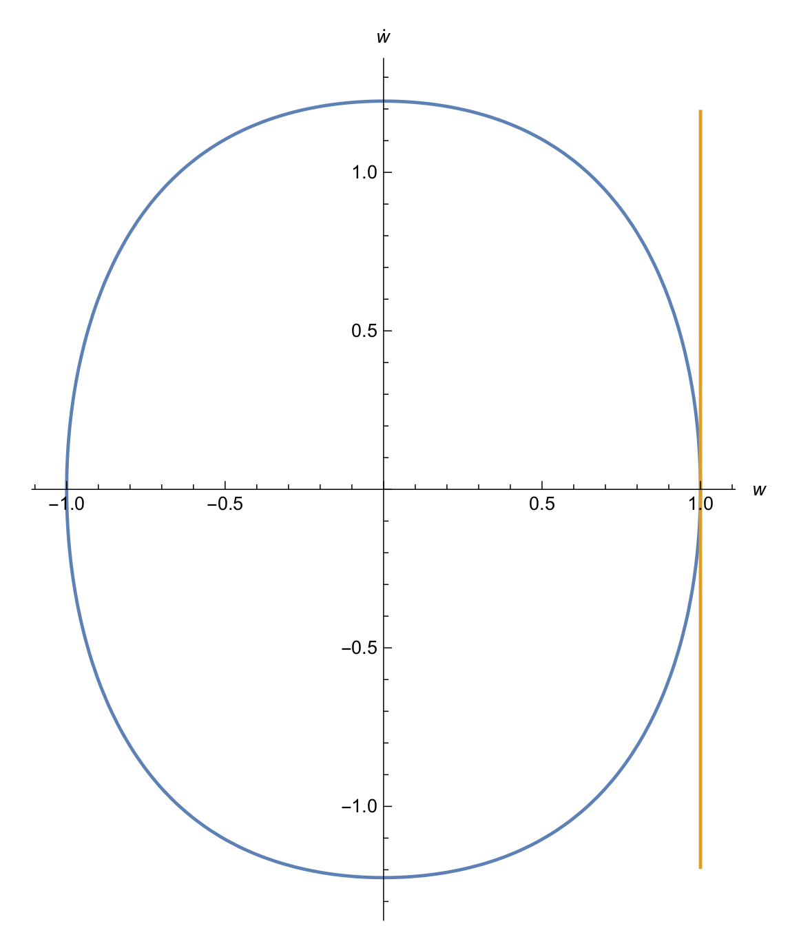
where is the complete elliptic integral of the first kind. To get impact (25), we need . When , we have a periodic grazing impact solution [20] (see Figure 1), so this solution is just touching the impact wall at for .
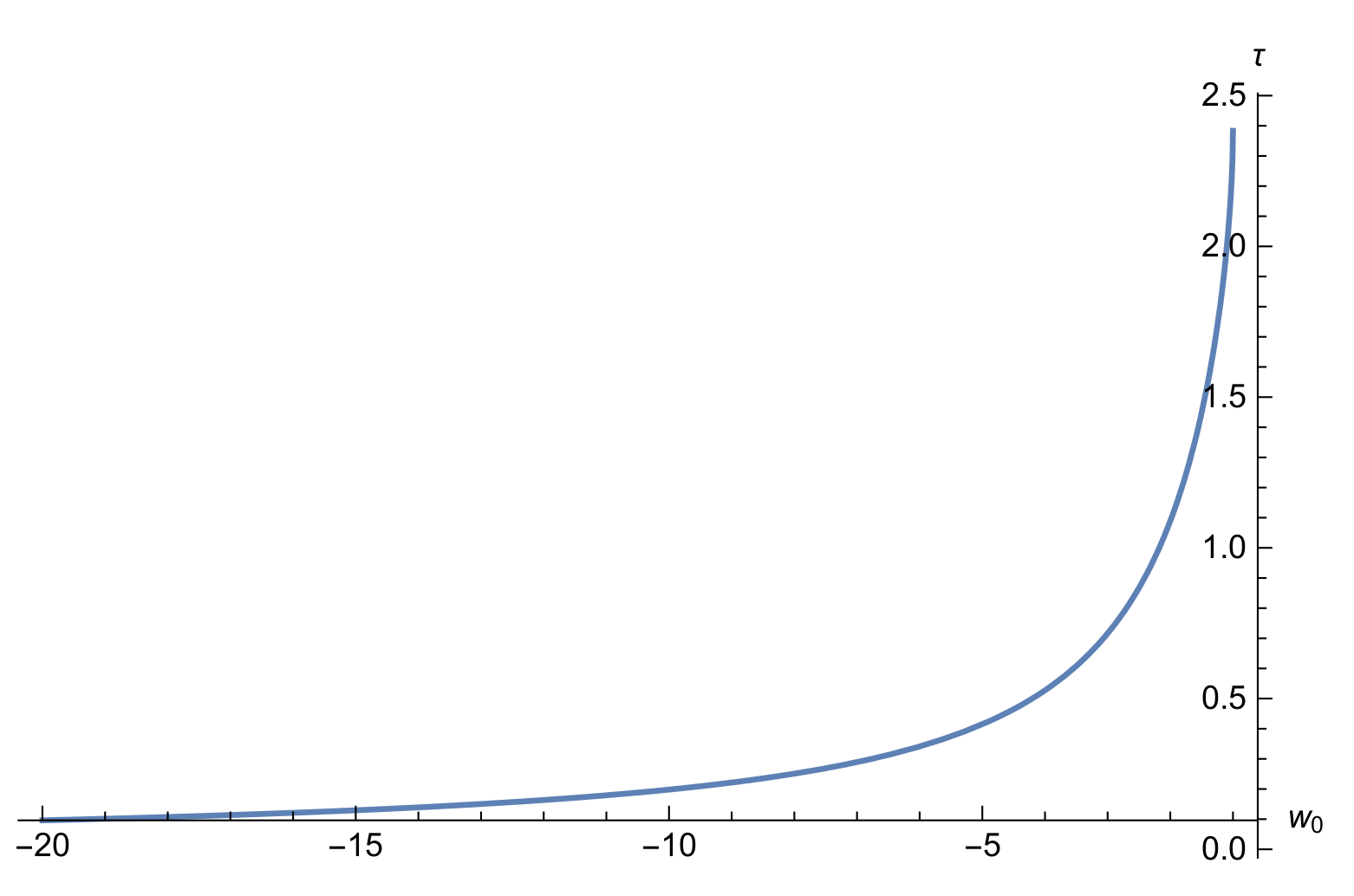
For , the impact time from Theorem 2 is given by , which means to solve
so
One can numerically check that is increasing with (see Figure 2).
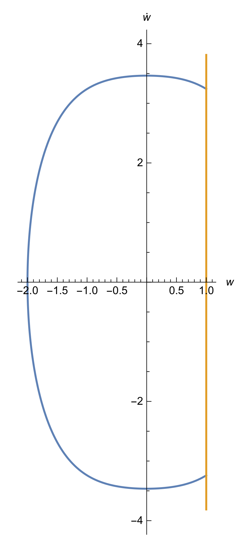
For any , we have periodic impact solutions; see Figure 3.
Consequently, we can apply Theorem 2 to (24) with (25) for any fixed , , to see that is -near to on for any sufficiently small. This means that we know -approximately dynamics of (24) with (25) on a time scale for any sufficiently small.
Similarly, we can investigate a weakly nonlinear and weakly periodically forced inverted pendulum with double impacts [21].
5. Conclusions
An averaging method was developed for weakly nonlinear and periodic second order differential equations subjected to impacts. Asymptotic estimation was derived between solutions of original and averaged equations. In this paper, we focused on the theoretical justification of the averaging principle for periodic second order differential equations and its applications to impact systems. The next step would be a numerical implementation of the above approach and method. This means an extension of averaging method for first order difference equations (see [22,23,24]) to second order ones, as in this paper, and a combination with discrete numerical schemes [25]. Another further direction would be dealt with more general discontinuous cases.
Author Contributions
Methodology, M.F.; investigation, J.P. All authors have read and agreed to the published version of the manuscript.
Funding
M.F. was partially supported by the Slovak Research and Development Agency under the contract number APVV-18-0308 and by the Slovak Grant Agency VEGA number 1/0358/20 and number 2/0127/20. J.P. was supported in part by VEGA grant 1/0347/18, by the Slovak Grant Agency VEGA number 1/0358/20 and by the Slovak Research and Development Agency under the contract number APVV-18-0308.
Conflicts of Interest
The authors declare no conflict of interest.
References
- Fiedler, B.; Scheurle, J. Discretization of Homoclinic Orbits, Rapid Forcing and “Invisible” Chaos. Mem. Am. Math. Soc. 1996, 119, 570. [Google Scholar] [CrossRef]
- Lombardi, E. Oscillatory Integrals and Phenomena Beyond all Algebraic Orders; Lecture Notes in Mathematics 1741; Springer: Berlin, Germany, 2000. [Google Scholar]
- Chicone, C. Ordinary Differential Equations with Applications, 2nd ed.; Texts in Applied Mathematics; Springer: New York, NY, USA, 2006. [Google Scholar]
- Hale, J.K. Ordinary Differential Equations; Wiley-Interscience: New York, NY, USA, 1969. [Google Scholar]
- Ricceri, B. A class of equations with three solutions. Mathematics 2020, 8, 478. [Google Scholar] [CrossRef] [Green Version]
- Treanţă, S. Gradient structures associated with a polynomial differential equation. Mathematics 2020, 8, 535. [Google Scholar] [CrossRef] [Green Version]
- Chow, S.N.; Hale, J.K. Methods of Bifurcation Theory; Springer: Berlin, Germany, 1982. [Google Scholar]
- Gao, P. Averaging principle for stochastic Korteweg-de Vries equation. J. Differ. Equ. 2019, 267, 6872–6909. [Google Scholar] [CrossRef]
- Guckenheimer, J.; Holmes, P.J. Nonlinear Oscillations, Dynamical Systems and Bifurcations of Vector Fields; Applied Mathematical Sciences; Springer: New York, NY, USA, 1983. [Google Scholar]
- Lehman, B.; Weibel, S.P. Fundamental theorems of averaging for functional differential equations. J. Differ. Equ. 1999, 152, 160–190. [Google Scholar] [CrossRef] [Green Version]
- Liu, W.; Röckner, M.; Sun, X.B.; Xie, Y.C. Averaging principle for slow-fast stochastic differential equations with time dependent locally Lipschitz coefficients. J. Differ. Equ. 2020, 268, 2910–2948. [Google Scholar] [CrossRef] [Green Version]
- Maslov, V.P. An averaging method for the quantum many-body problem. Funct. Anal. Its Appl. 1999, 33, 280–291. [Google Scholar] [CrossRef]
- Murdock, J.A.; Sanders, J.A.; Verhulst, F. Averaging Methods in Nonlinear Dynamical Systems; Applied Mathematical Sciences; Springer Science+Business Media, LLC: New York, NY, USA, 2007. [Google Scholar]
- Zgliczyński, P. Hyperbolicity and averaging for the Srzednicki–Wójcik equation. J. Differ. Equ. 2017, 262, 1931–1955. [Google Scholar] [CrossRef] [Green Version]
- Bernardo, M.; Budd, C.; Champneys, A.R.; Kowalczyk, P. Piecewise-Smooth Dynamical Systems: Theory and Applications; Applied Mathematical Sciences; Springer: London, UK, 2008. [Google Scholar]
- Battelli, F.; Fečkan, M. Chaos in forced impact systems. Disc. Cont. Dyn. Syst. S 2013, 6, 861–890. [Google Scholar] [CrossRef]
- Fečkan, M.; Pačuta, J.; Pospíšil, M.; Vidlička, P. Averaging methods for piecewise-smooth ordinary differential equations. AIMS Math. 2019, 4, 1466–1487. [Google Scholar]
- Liu, K.; Fečkan, M.; Wang, J.R. A fixed point approach to the Hyers-Ulam stability of Caputo-Fabrizio fractional differential equations. Mathematics 2020, 8, 647. [Google Scholar] [CrossRef] [Green Version]
- Lawden, D.F. Elliptic Functions and Applications; Springer: New York, NY, USA, 1989. [Google Scholar]
- Battelli, F.; Fečkan, M. On the Poincaré-Adronov-Melnikov method for the existence of grazing impact periodic solutions of differential equations. J. Differ. Equ. 2020, 268, 3725–3748. [Google Scholar] [CrossRef]
- Shen, J.; Du, Z.D. Double impact periodic orbits for an inverted pendulum. Int. J. Non Linear Mech. 2011, 46, 1177–1190. [Google Scholar] [CrossRef]
- Belan, V.G. Averaging method for difference equations. Ukr. Mat. Zhurnal 1976, 28, 78–82. [Google Scholar]
- Brännström, N. Averaging in weakly coupled discrete dynamical systems. J. Nonlinear Math. Phys. 2009, 16, 465–487. [Google Scholar] [CrossRef]
- Martynyuk, D.I.; Danilov, V.Y.; Panikov, V.G. On the second Bogolyubov theorem for a system of difference equations. Ukr. Mat. Zhurnal 1988, 40, 110–120. [Google Scholar] [CrossRef]
- Griffiths, D.F.; Higham, D.J. Numerical Methods for Ordinary Differential Equations; Springer: London, UK, 2010. [Google Scholar]

Figure 2.
The graph of (28) on .
Figure 2.
The graph of (28) on .


© 2020 by the authors. Licensee MDPI, Basel, Switzerland. This article is an open access article distributed under the terms and conditions of the Creative Commons Attribution (CC BY) license (http://creativecommons.org/licenses/by/4.0/).
Share and Cite
MDPI and ACS Style
Fečkan, M.; Pačuta, J. Averaging Methods for Second-Order Differential Equations and Their Application for Impact Systems. Mathematics 2020, 8, 916. https://0-doi-org.brum.beds.ac.uk/10.3390/math8060916
AMA Style
Fečkan M, Pačuta J. Averaging Methods for Second-Order Differential Equations and Their Application for Impact Systems. Mathematics. 2020; 8(6):916. https://0-doi-org.brum.beds.ac.uk/10.3390/math8060916
Chicago/Turabian StyleFečkan, Michal, and Július Pačuta. 2020. "Averaging Methods for Second-Order Differential Equations and Their Application for Impact Systems" Mathematics 8, no. 6: 916. https://0-doi-org.brum.beds.ac.uk/10.3390/math8060916
Note that from the first issue of 2016, this journal uses article numbers instead of page numbers. See further details here.