Normal Partner Curves of a Pseudo Null Curve on Dual Space Forms


1
Department of Mathematics, Northeastern University, Shenyang 110004, China
2
Department of Mathematics, Kyungpook National University, Daegu 41566, Korea
*
Author to whom correspondence should be addressed.
Mathematics 2020, 8(6), 919; https://0-doi-org.brum.beds.ac.uk/10.3390/math8060919
Submission received: 4 May 2020
/
Revised: 30 May 2020
/
Accepted: 1 June 2020
/
Published: 5 June 2020
(This article belongs to the Special Issue Computer Aided Geometric Design)
Abstract
:In this work, a kind of normal partner curves of a pseudo null curve on dual space forms is defined and studied. The Frenet frames and curvatures of a pseudo null curve and its associate normal curve on de-Sitter space, its associate normal curve on hyperbolic space, are related by some particular function and the angles between their tangent vector fields, respectively. Meanwhile, the relationships between the normal partner curves of a pseudo null curve are revealed. Last but not least, some examples are given and their graphs are plotted by the aid of a software programme.
1. Introduction
In differential geometry, the space associate curves for which there exist some relations between their Frenet frames or curvatures compose a large class of fascinating subjects in the curve theory, such as Bertrand curve, Mannheim curve, central trace of osculating sphere, involute-evolute curves etc. [1,2,3]. Most of the researchers aimed to explore the relationships between the partner curves. For example, in Euclidean 3-space, the classical Bertrand curves are characterized by constant distance between the corresponding points of the partner curves and by constant angle between tangent vector fields of the partner curves. Naturally, the idea of partner curves research can be moved to other spaces, such as Lorentz-Minkowski space, Galilean space and so on.
The Lorentz-Minkowski metric divides the vectors into spacelike, timelike and lightlike (null) vectors [4]. Due to the causal character of vectors, some simple problems become a little complicated and strange, such as the arc-length of null curves can not be defined similar to the definition in Euclidean space; the angles between different type of vectors need to be classified according to different conditions [5,6]. In Minkowski space, the curves are divided into spacelike, timelike and lightlike (null) curves according to the causal character of their tangent vectors. Some particular curves such as the helix, the Bertrand curve, the Mannheim curve and the normal curve, the osculating curve and the rectifying curve have been surveyed by some researchers [5,7,8,9,10,11,12].
Based on pseudo null curves in Minkowski 3-space, in this work, we define a kind of normal partner curves of a pseudo null curve which lies on de-Sitter space and hyperbolic space, respectively. In Section 2, some fundamental facts about the pseudo null curves, the space forms and the angles between any two non-null vectors are recalled. In Section 3, the relationships between a pseudo null curve and its normal partner curves on dual space forms are explicitly expressed by some particular function and the angles between their tangent vector fields. Furthermore, the relationships between the normal partner curves of a pseudo null curve are presented through the pseudo null curve. Last but not least, some useful and interesting examples of pseudo null curves and their normal partner curves are shown vividly.
The curves in this paper are regular and smooth unless otherwise stated.
2. Preliminaries
The Minkowski 3-space is provided with the standard indefinite flat metric given by
in terms of the natural coordinate system . Recall that a vector v is said to be spacelike, timelike and lightlike (null), if or , and , , respectively. The norm (modulus) of v is defined by . For any two vectors , , the vector product is given by
where is an orthogonal basis in .
An arbitrary curve can locally be spacelike, timelike or lightlike (null) if all of its velocity vectors are spacelike, timelike or lightlike, respectively. Furthermore, the spacelike curves can be classified into three kinds according to their principal normal vectors are spacelike, timelike or lightlike, which are called the first and the second kind of spacelike curve and the pseudo null curve, respectively [13]. Among of them, the pseudo null curve is defined as the following.
Definition 1.
([6]). A spacelike curve framed by Frenet frame in is called a pseudo null curve, if its principal normal vector N and binormal vector B are linearly independent lightlike (null) vectors.
Proposition 1.
([6]). Let be a pseudo null curve parameterized by arc-length s, i.e., . Then there exists a unique Frenet frame such that
where and In sequence, is called the tangent, principal normal and binormal vector fields of , respectively. The function is called the pseudo null curvature of .
Remark 1.
([8]). Every pseudo null curve in is planar no matter the value of the pseudo null curvature.
The authors of [14] characterized pseudo null curves with the structure function as the following.
Proposition 2
and
where , is non-constant function which is called the structure function of .
Definition 2
([15]). Let p be a fixed point in and be a constant. Then the pseudo-Riemannian space forms, i.e., the de-Sitter space , the hyperbolic space and the lightlike cone are defined as
The point p is called the center of , and . When p is the origin and , we simply denote them by , and .
For a pseudo null curve framed by in , the planes spanned by , and are known as the osculating, the rectifying and the normal planes of , respectively. A curve is called an associate osculating, an associate rectifying, or an associate normal curve of when the position vector always lies on the osculating, the rectifying, or the normal plane of , respectively. For an associate normal curve of a pseudo null curve , we can write
for some non-zero differentiable functions and . In particular, if the associate normal curve lies on or , then and satisfy or . Without lose of generality, we have the following definition.
Definition 3.
Let be a pseudo null curve framed by in . Then , is called an associate normal curve of on de-Sitter space, an associate normal curve of on hyperbolic space for some non-zero differentiable function , respectively. In a word, and are called normal partner curves of on dual space forms.
To serve the discussions, some fundamental facts of curves lying on space forms will be reviewed.
Proposition 3
([15]). Let be a curve parameterized by arc-length s. Then there exists a unique pseudo spherical Frenet frame such that
where , The function is called the pseudo spherical curvature of .
Proposition 4
([15]). Let be a curve parameterized by arc-length s. Then there exists a unique hyperbolic Frenet frame such that
where , The function is called the hyperbolic curvature of .
At last, let us recall the notion of angles between two arbitrary non-null vectors in .
Definition 4
([16]). Let u and v be spacelike vectors in .
- If u and v span a timelike vector subspace. Then we have and hence, there is a unique positive real number θ such thatThe real number θ is called the Lorentz timelike angle between u and v.
- If u and v span a spacelike vector subspace. Then we have and hence, there is a unique real number such thatThe real number θ is called the Lorentz spacelike angle between u and v.
Definition 5
([16]). Let u be a spacelike vector and v a future pointing timelike vector in . Then there is a unique non-negative real number θ such that
The real number θ is called the Lorentz timelike angle between u and v.
Definition 6.
[16] Let u and v be future pointing (past pointing) timelike vectors in . Then there is a unique non-negative real number θ such that
The real number θ is called the Lorentz timelike angle between u and v.
Remark 2
Remark 3.
The angles between a lightlike vector and an arbitrary spacelike vector, timelike vector or another lightlike vector which is independent to it have been defined in [6]. We do not recall the details here, because they are not involved in this paper.
3. Main Conclusions
In this section, the associate normal curves of a pseudo null curve on de-Sitter space and hyperbolic space, respectively will be discussed. At the same time, the relationships between the normal partner curves will be presented.
3.1. Associate Normal Curves of a Pseudo Null Curve on de-Sitter Space
Let be a pseudo null curve framed by , its associate normal curve on de-Sitter space framed by . From Proposition 3, we have
Case (1): , i.e., is spacelike. In order to distinguish different cases, we rewrite Equation (2) as the following:
where is the arc-length of , and ,
Taking derivative on both sides of with respect to the arc-length s of , we get
where . Making inner product on both sides of Equation (8) with itself, we get . Then, we have
substituting it into Equation (8), we get
Due to are spacelike vectors and is spacelike, then T and span a timelike subspace. According to Equation (4), we have
where is the Lorentz timelike angle between T and . Together with , we get , thus . Explicitly, when , ; when , . Then, Equation (10) can be rewritten as
Taking inner product on both sides of Equation (12) with itself, we get
considering and , by Equation (13) we have
Case (2): , i.e., is timelike. Similar to the process of Case 1, we can rewrite Equation (2) as the following:
where is the arc-length of , and ,
Taking derivative on both sides of with respect to the arc-length s of , we get
where . Making inner product on both sides of Equation (15) with itself, we get . Then, we have
substituting it into Equation (15), we get
Due to T is spacelike, is timelike, according to Equation (6), we have
where is the Lorentz timelike angle between T and Together with , we get thus (). Explicitly, when , ; when , . Then, Equation (17) can be rewritten as
Taking inner product on both sides of Equation (19) with itself, we get
considering and by Equation (20) we have
Based on above discussions, we can get the following conclusions.
Theorem 1.
Let be a pseudo null curve framed by , its associate normal curve on de-Sitter space framed by .
- If is spacelike, then the Frenet frame of and the pseudo spherical Frenet frame of can be related by asor the Lorentz timelike angle between T and aswhere , , and when , ; when , .
- If is timelike, then the Frenet frame of and the pseudo spherical Frenet frame of can be related by asor the Lorentz timelike angle between T and aswhere , , and when , ; when , .
Theorem 2.
Let be a pseudo null curve framed by , its associate normal curve on de-Sitter space framed by .
- If is spacelike, the pseudo spherical curvature of can be expressed by
- If is timelike, the pseudo spherical curvature of can be expressed by
where ϵ, , and f as stated in Theorem 1.
It is obvious that the case is excluded in the first case of Theorems 1 and 2. In fact, when , i.e., , by solving the differential equation, we get
Furthermore, from Equation (1), by substituting into above equation, we have
Corollary 1.
Let be a pseudo null curve framed by with pseudo null curvature and structure function , its associate normal curve on de-Sitter space framed by . If , then we have
- the arc-length of can be expressed by ;
- the pseudo spherical curvature of is ;
- the Frenet frame of and the pseudo spherical Frenet frame of can be related by
Proof of Corollary 1.
When , by taking derivative on both sides of with respect to the arc-length s of , we get
Making inner product on both sides of Equation (22) with itself, we get . Then, we get
Making inner product on both sides of Equation (25) with itself, we have . Then from and Equation (25), we can obtain
The proof is completed. □
Remark 4.
Obviously, the corresponding results in Theorems 1 and 2 still hold for , i.e., .
3.2. Associate Normal Curves of a Pseudo Null Curve on Hyperbolic Space
Let be a pseudo null curve framed by , its associate normal curve on hyperbolic space framed by . From Proposition 4, we can rewrite Equation (3) as the following:
where is the arc-length of , and ,
Taking derivative on both sides of with respect to the arc-length s of , we get
where . Making inner product on both sides of Equation (26) with itself, we get . Then, we have
substituting it into Equation (26), we get
Due to are spacelike vectors and is timelike, then T and span a spacelike subspace. According to Equation (5), we have
where is the Lorentz spacelike angle between T and . Together with , we can get , thus Explicitly, when ; when . Then, Equation (28) can be rewritten as
Taking inner product on both sides of Equation (30) with itself, we get
considering and , by Equation (31) we have
Summarize above discussions, we have the following conclusions.
Theorem 3.
Let be a pseudo null curve framed by , its associate normal curve on hyperbolic space framed by . Then the Frenet frame of and the hyperbolic Frenet frame of can be related by as
or the Lorentz spacelike angle between T and as
where , , and when ; when .
Theorem 4.
Let be a pseudo null curve framed by , its associate normal curve on hyperbolic space framed by . Then the hyperbolic curvature of can be expressed by
where ϵ, , and f as stated in Theorem 3.
Similar to the procedure of the associate normal curve of a pseudo null curve on de-Sitter space , for the associate normal curve of a pseudo null curve on hyperbolic space , when , i.e., , we have the following conclusions.
Corollary 2.
Let be a pseudo null curve framed by with pseudo null curvature and structure function , its associate normal curve on hyperbolic space framed by . If , then we have
- the arc-length of can be expressed by ;
- the hyperbolic curvature of is ;
- the Frenet frame of and the hyperbolic Frenet frame of can be related by
Remark 5.
The proof of Corollary 2 is omitted here since it is very similar to Corollary 1. Obviously, the results in Theorems 3 and 4 still hold for , i.e., .
3.3. The Relationships of the Normal Partner Curves
In this section, we state the relations of the normal partner curves on dual space forms using the knowledge of linear algebra and the results obtained in Section 3.1 and Section 3.2.
Theorem 5.
Let be a pseudo null curve framed by , framed by and framed by be normal partner curves of on dual space forms.
- If is spacelike, then the pseudo spherical Frenet frame of and the hyperbolic Frenet frame of can be related by asor the Lorentz timelike angle between T and , the Lorentz spacelike angle between T and aswhere , , and , as stated in Theorems 1 and 3, respectively. and when , ; when , .
- If is timelike, then the pseudo spherical Frenet frame of and the hyperbolic Frenet frame of can be related by asor the Lorentz timelike angle between T and , the Lorentz spacelike angle between T and as
where , , and , as stated in Theorems 1 and 3, respectively. and when , ; when , .
Proof of Theorem 5.
From Theorems 1 and 3, by some matrix calculations, it is easy to get the conclusions. □
At the same time, from Theorems 2 and 4, the following conclusions are straightforward.
Theorem 6.
Let be a pseudo null curve framed by , framed by and framed by be normal partner curves of on dual space forms. Then the pseudo spherical curvature of and the hyperbolic curvature of satisfy
- if is spacelike, , then we haveand they are related by , when , ; when , . and as stated in Theorems 1 and 3, respectively;
- if is timelike, , then we haveand they are related by when , ; when , . and as stated in Theorems 1 and 3, respectively.
Considering Corollaries 1 and 2, when , i.e., , we have the following conclusions.
Corollary 3.
Let be a pseudo null curve framed by with pseudo null curvature and structure function , framed by and framed by be normal partner curves of on dual space forms. If , then we have
- the arc-length of and all can be expressed by ;
- the pseudo spherical curvature of and the hyperbolic curvature of satisfy
- the pseudo spherical Frenet frame of and the hyperbolic Frenet frame of can be related by
Remark 6.
In Corollaries 1–3, for a given pseudo null curve , when the smooth function , the pseudo spherical curvature of and the hyperbolic curvature of . How about the converse statement? i.e., when a pseudo spherical curve with spacelike normal vector field has pseudo spherical curvature or a hyperbolic curve has hyperbolic curvature , how to find out the corresponding pseudo null curve and what is the relationship between the smooth function and the null curvature function or the structure function of ? These problems are still in the air and can be considered in the future.
4. Examples
Example 1.
Consider a pseudo null curve framed by whose curvature is . From the Frenet formula of , then we know
Example 2.
Consider a pseudo null curve framed by whose curvature is . From the Frenet formula of , then we know
Author Contributions
J.Q. and X.T. set up the problem and computed the details. Y.H.K. checked and polished the draft. All authors have read and agreed to the published version of the manuscript.
Funding
The first author was supported by NSFC (No. 11801065) and the Fundamental Research Funds for the Central Universities (N2005012). The third author was supported by the National Research Foundation of Korea(NRF) grant funded by the Korea Government (NRF-2019R1H1A2079891).
Acknowledgments
We thank H. Liu of Northeastern University and the referee for the careful review and the valuable comments to improve the paper.
Conflicts of Interest
The authors declare no conflict of interest.
References
- Liu, H.L.; Wang, F. Mannheim partner curves in 3-space. J. Geom. 2008, 11, 25–31. [Google Scholar] [CrossRef]
- Tuncer, Y.; Sperpil, U. New representations of Bertrand pairs in Euclidean 3-space. Appl. Math. Comput. 2012, 219, 1833–1842. [Google Scholar]
- Yuce, S.; Kuruoglu, N.; Kasap, E. The involute-evolute offsets of ruled surfaces. Iran. J. Sci. Technol. A 2009, 33, 195–201. [Google Scholar]
- Ali, A.T.; Turgut, M. Position vector of a timelike slant helix in Minkowski 3-space. J. Math. Anal. Appl. 2010, 365, 559–569. [Google Scholar] [CrossRef] [Green Version]
- Qian, J.H.; Kim, Y.H. Directional associated curves of a null curve in . Bull. Korean Math. Soc. 2015, 52, 183–200. [Google Scholar] [CrossRef]
- Qian, J.H.; Tian, X.Q.; Liu, J.; Kim, Y.H. A new angular measurement in Minkowski 3-Space. Mathematics 2020, 8, 56. [Google Scholar] [CrossRef] [Green Version]
- Choi, J.H.; Kang, T.H.; Kim, Y.H. Bertrand curves in 3-dimensional space forms. Appl. Math. Comput. 2012, 219, 1040–1046. [Google Scholar] [CrossRef]
- Da Silva, L.C.B. Moving frames and the characterization of curves that lie on a surface. J. Geom. 2017, 108, 1091–1113. [Google Scholar] [CrossRef]
- Liu, H.L. Curves in the lightlike cone. Contrib. Alg. Geom. 2004, 45, 291–303. [Google Scholar]
- Lucas, P.; Ortega-Yagues, J.A. Rectifying curves in the three-dimensional sphere. J. Math. Anal. Appl. 2015, 421, 1855–1868. [Google Scholar] [CrossRef]
- Nesovic, E.; Ozturk, U.; Ozturk, E.B.K. On k-type pseudo null Darboux helices in Minkowski 3-space. J. Math. Anal. Appl. 2016, 439, 690–700. [Google Scholar] [CrossRef]
- Ali, U.; Osman, K.; Kazim, I. Generalized Bertrand curves with timelike (1,3)-normal plane in Minkowski space-time. Kuwait J. Sci. 2015, 42, 10–27. [Google Scholar]
- O’Neill, B. Semi-Riemannian Geometry with Applications to Relativity; Academic Press: Cambridge, MA, USA, 1983; Volume 103, pp. 310–312. [Google Scholar]
- Qian, J.H.; Liu, J.; Tian, X.Q.; Kim, Y.H. Structure functions of pseudo null curves in Minkowski 3-Space. Mathematics 2020, 8, 75. [Google Scholar] [CrossRef] [Green Version]
- Liu, H.L.; Yuan, Y. Pitch functions of ruled surfaces and B-scrolls in Minkowski 3-space. J. Geom. Phys. 2012, 62, 47–52. [Google Scholar] [CrossRef]
- Fu, Y.; Wang, X.S. Classification of timelike constant slope Surfaces in 3-Dimensional Minkowski spaces. Results Math. 2013, 63, 1095–1108. [Google Scholar] [CrossRef]
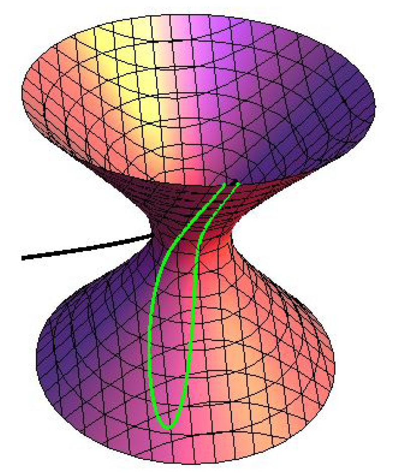
Figure 1.
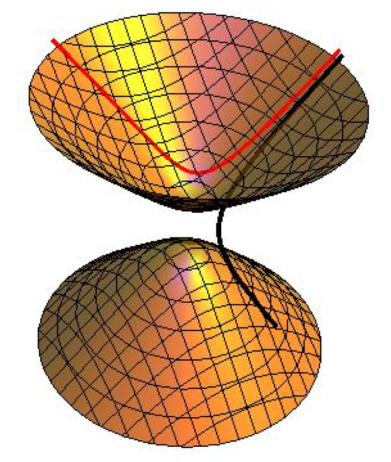
(black) and (green) in Example 1.

Figure 2.
(black) and (red) in Example 1.

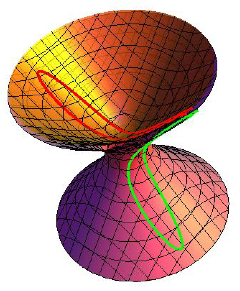
Figure 3.
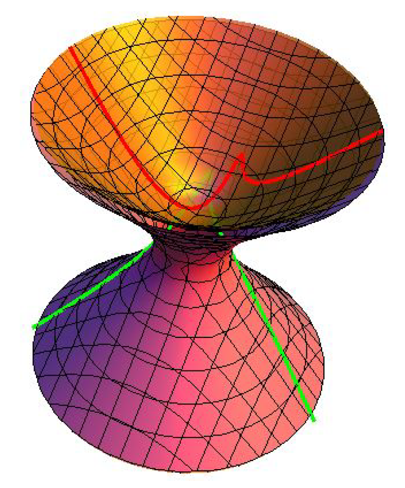
(green) and (red) in Example 1.

Figure 4.
(black) and (green) in Example 2.

Figure 5.
(black) and (red) in Example 2.

Figure 6.
(green) and (red) in Example 2.

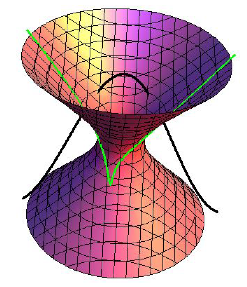
Figure 7.
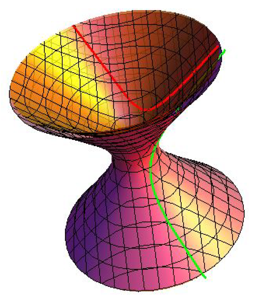
(black) and (green) in Example 3.

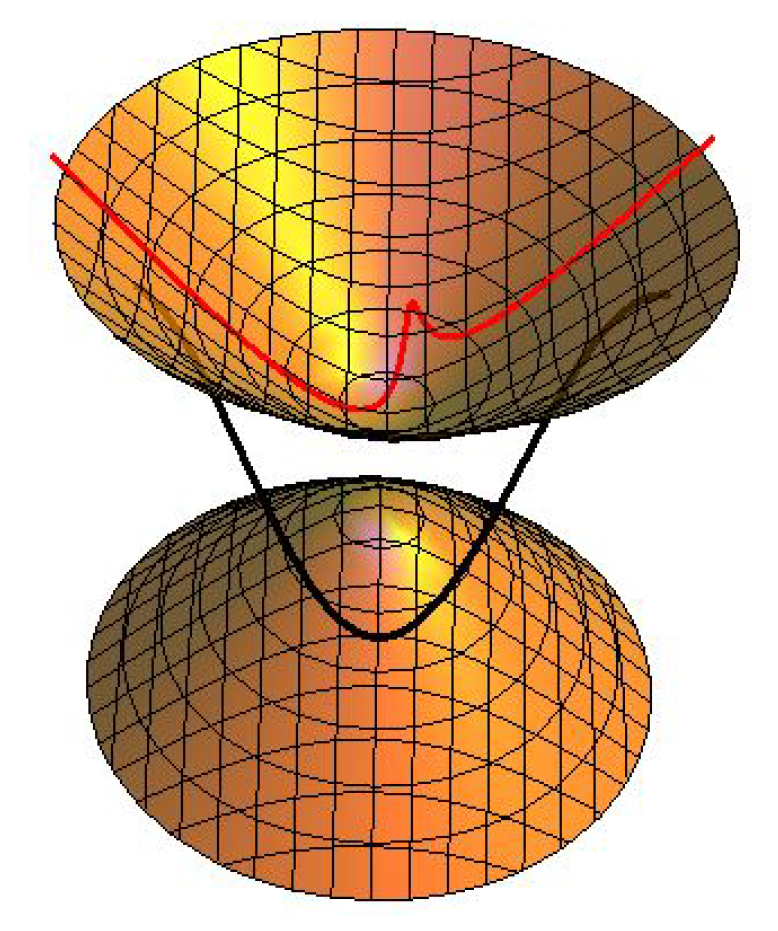
Figure 8.
(black) and (red) in Example 3.

Figure 9.
(green) and (red) in Example 3.

© 2020 by the authors. Licensee MDPI, Basel, Switzerland. This article is an open access article distributed under the terms and conditions of the Creative Commons Attribution (CC BY) license (http://creativecommons.org/licenses/by/4.0/).
Share and Cite
MDPI and ACS Style
Qian, J.; Tian, X.; Kim, Y.H. Normal Partner Curves of a Pseudo Null Curve on Dual Space Forms. Mathematics 2020, 8, 919. https://0-doi-org.brum.beds.ac.uk/10.3390/math8060919
AMA Style
Qian J, Tian X, Kim YH. Normal Partner Curves of a Pseudo Null Curve on Dual Space Forms. Mathematics. 2020; 8(6):919. https://0-doi-org.brum.beds.ac.uk/10.3390/math8060919
Chicago/Turabian StyleQian, Jinhua, Xueqian Tian, and Young Ho Kim. 2020. "Normal Partner Curves of a Pseudo Null Curve on Dual Space Forms" Mathematics 8, no. 6: 919. https://0-doi-org.brum.beds.ac.uk/10.3390/math8060919
Note that from the first issue of 2016, this journal uses article numbers instead of page numbers. See further details here.