Article

A New Modified Kies Family: Properties, Estimation Under Complete and Type-II Censored Samples, and Engineering Applications

by
Abdulhakim A. Al-Babtain
1,
Mohammed K. Shakhatreh
2,
Mazen Nassar
3,4 and
Ahmed Z. Afify
5,*
1
Department of Statistics and Operations Research, King Saud University, Riyadh 11362, Saudi Arabia
2
Department of Mathematics and Statistics, Jordan University of Science and Technology, P.O. Box 3030, Irbid 22110, Jordan
3
Department of Statistics, Faculty of Science, King Abdulaziz University, Jeddah 21589, Saudia Arabia
4
Department of Statistics, Faculty of Commerce, Zagazig University, Zagazig 44511, Egypt
5
Department of Statistics, Mathematics and Insurance, Benha University, Benha 13511, Egypt
*
Author to whom correspondence should be addressed.
Submission received: 27 July 2020 / Revised: 7 August 2020 / Accepted: 9 August 2020 / Published: 12 August 2020
(This article belongs to the Special Issue Probability, Statistics and Their Applications)

Abstract

:
In this paper, we introduce a new family of continuous distributions that is called the modified Kies family of distributions. The main mathematical properties of the new family are derived. A special case of the new family has been considered in more detail; namely, the two parameters modified Kies exponential distribution with bathtub shape, decreasing and increasing failure rate function. The importance of the new distribution comes from its ability in modeling positively and negatively skewed real data over some generalized distributions with more than two parameters. The shape behavior of the hazard rate and the mean residual life functions of the modified Kies exponential distribution are discussed. We use the method of maximum likelihood to estimate the distribution parameters based on complete and type-II censored samples. The approximate confidence intervals are also obtained under the two schemes. A simulation study is conducted and two real data sets from the engineering field are analyzed to show the flexibility of the new distribution in modeling real life data.

1. Introduction

In the last few decades, there have been an increased interest among statisticians to define new families of distributions by adding extra shape parameter (one or more) to a baseline distribution. The extra parameters of a good generator can usually give lighter tails and heavier tails, accommodate symmetric, unimodal, bimodal, right-skewed and left-skewed density function, and increase and decrease skewness and kurtosis and, more important, yield all types of the hazard function. Furthermore, the extra parameters can provide great flexibility for modelling data in several areas such as economics, engineering, reliability and medical sciences, among others. Kumar and Dharmaja [1] proposed the reduced Kies distribution as a special case of the Kies distribution. Here, we will refer to the reduced Kies distribution as the modified Kies (MKi) distribution. The cumulative distribution function (CDF) of the MKi distribution is specified (for 0 < t < 1 ) by
F ( t ) = 1 exp t 1 t a .
Its probability density function (PDF) takes the form
f ( t ) = a t a 1 1 t a 1 exp t 1 t a ,
respectively, where a > 0 is a shape parameter. Kumar and Dharmaja [1] observed that the MKi distribution perform better than the Weibull distribution and some of its extensions in modelling data. Kumar and Dharmaja [2] introduced the exponentiated reduced Kies distribution and studied some properties of the distribution. Dey et al. [3] derived the recurrence relations for the single and product moments of the MKi distribution under progressive type-II censoring scheme as well as the estimation of the distribution parameters.
In this paper, we propose a new family of distributions based on the MKi distribution. In fact, based on the T-X family pioneered by Alzaatreh et al. [4], we construct a new generator so-called the modified Kies generalized(MKi-G) family. Given a baseline distribution, the MKi-G distribution can be used effectively for analysis purposes.
If G ( x ; ξ ) is the baseline CDF depending on a parameter vector ξ , then the CDF of the MKi-G family is defined by
F ( x ; a , ξ ) = 0 G ( x ; ξ ) a t a 1 1 t a 1 exp t 1 t a d t = 1 exp G ( x ; ξ ) 1 G ( x ; ξ ) a , x > 0 , a > 0 .
The corresponding PDF of (1) is given by
f x ; a , ξ = a g ( x ; ξ ) G ( x ; ξ ) a 1 1 G ( x ; ξ ) a + 1 exp G ( x ; ξ ) 1 G ( x ; ξ ) a .
The hazard rate (HR) function of the MKi-G family is given by
h x ; a , ξ = a g ( x ; ξ ) G ( x ; ξ ) a 1 1 G ( x ; ξ ) a + 1 .
Henceforth, a random variable with density function (2) is denoted by X∼MKi- G a , ξ .
The main aim of this paper is to introduce and study a new family of distributions which called the modified Kies-G (MKi-G) family. We discuss some general mathematical properties of MKi-G family. Although the MKi distribution proposed by [1] has interesting properties, it is not flexible in modeling real data because it does not contain a scale parameter. An extended model including a scale parameter has considered by taking the exponential distribution as baseline for the MKi-G family and generate a two-parameter MKi-exponential (MKiEx) distribution, which has several desirable properties. The MKiEx distribution has a very flexible PDF, it can be positive skewed, negative skewed and symmetric, and can allow for greater flexibility of the tails. It is capable of modeling monotonically decreasing, increasing and bathtub hazard rates. Moreover, it has a closed form CDF and very easy to handle which make the distribution is candidate to use in different fields such as life testing, reliability, biomedical studies and survival analysis. Two real data applications show that the proposed distribution is very competitive to some traditional distributions with scale and shape parameters like Weibull and gamma distributions. It can also be considered as a good alternative to some recently introduced distributions such as the alpha power exponential distribution (APE) by Mahdavi and Kundu [5], generalized odd log-logistic exponential distribution by Afify et al. [6], and extended odd Weibull exponential distribution by Afify and Mohamed [7].
The rest of this paper is organized as follows: in Section 2, we obtain some mathematical properties of the MKi-G family. In Section 3, we introduce the MKiEx distribution. Some mathematical properties of the hazard rate function of the MKiEx distribution are derived in Section 4. The Asymptotic distributions of order statistics of the MKiEx distribution are shown in Section 5. In Section 6, we study the mean residual life of the MKiEx distribution. In Section 7, the maximum likelihood estimates and the approximate confidence intervals are obtained under complete and type-II censored samples as well as the simulation study. The analysis of two real data sets are presented in Section 8. The paper is concluded in Section 9.

2. Properties of the MKi Generator

In this section, we obtain some mathematical properties of the MKi-G family such as mixture representation, quantiles, moments, moment generating function (MGF), order statistics, probability weighted moments (PWMs), and Rényi entropy.

2.1. Mixture Representation

Using the exponential series and the power series,
1 z q + 1 = k = 0 q + k k z k , for | z | < 1 ,
we obtain a useful linear representation for the PDF (2) as
f x = j , k = 0 υ j , k h j + 1 a + k ( x ) ,
where h j + 1 a + k ( x ) denotes the exponentiated-G (exp-G) PDF with power parameter j + 1 a + k , and the coefficient υ j , k is given by
υ j , k = a 1 j j ! j + 1 a + k j + 1 a + k k .
Equation (4) gives the MKi-G family PDF as a linear combination of exp-G PDFs and enable us to derive some mathematical properties of the MKi-G family using this representation. More details about the exp-G distributions can be explored in Lemonte et al. [8].
Integrating (4), the CDF of X is given by
F x = j , k = 0 υ j , k H j + 1 a + k ( x ) ,
where H j + 1 a + k ( x ) is the CDF of the exp-G family with power parameter j + 1 a + k .

2.2. Quantiles, Ordinary and Incomplete Moments

The quantile function (QF) of (1) is given by
x p = Q M K i G ( p ) = G 1 log 1 p 1 a 1 + log 1 p 1 a .
A random sample of size n from (1) can be obtained, based on (5), as X i = Q M K i G ( U i ) , where U i Uniform( 0 , 1 ), i = 1 , , n .
Henceforth, Y j + 1 a + k denotes a random variable having the exp-G distribution with power parameter j + 1 a + k .
The rth moment of the MKi-G family can be derived from (4) as
μ r = E X r = j , k = 0 υ j , k E Y j + 1 a + k r .
The sth incomplete moment of X can be expressed from (4) as
φ s t = j , k = 0 υ j , k t x s h j + 1 a + k ( x ) d x .
The first incomplete moment, φ 1 t , follows from the last equation with s = 1 . The main applications of φ 1 t refers to the mean deviations and the Bonferroni and Lorenz curves (see, Lorenz [9] and Bonferroni [10]).

2.3. Generating Function

In this section, we provide two formulae for the MGF of X. The first one follows from Equation (4)
M X t = j , k = 0 υ j , k M j + 1 a + k t ,
where M j + 1 a + k t is the MGF of the random variable Y j + 1 a + k . Hence, M X t can be determined from the exp-G MGF. The second formula can also be derived from (4) by considering u = G x ; ξ . Therefore, the MGF can be represented as
M X t = j , k = 0 υ j , k τ t , k ,
where τ t , k = 0 1 exp t Q G u u j + 1 a + k 1 d u and Q G ( u ) is the QF corresponding to G x ; ξ , i.e., Q G ( u ) = G 1 ( u ; ξ ) .

2.4. Order Statistics

Let X 1 , , X n be a random sample from the MKi-G family. The PDF of the ith order statistic, X i , is defined by
f X i x = f x B i , n i + 1 j = 0 n i 1 j n i j F j + i 1 x ,
where B ( · , · ) is the beta function.
Based on Equation (1), we have
F j + i 1 ( x ) = m = 0 j + i 1 1 m j + i 1 m exp m G ( x ; ξ ) 1 G ( x ; ξ ) a .
Using (2) and the exponential series, we obtain
f x F j + i 1 ( x ) = m = 0 j + i 1 l = 0 1 m + l l ! m + 1 l j + i 1 m a g ( x ; ξ ) G ( x ; ξ ) l + 1 a 1 1 G ( x ; ξ ) l + 1 a + 1 .
After a power series expansion (3), we can write
f x F j + i 1 ( x ) = m = 0 j + i 1 l , k = 0 1 m + l l ! a m + 1 l j + i 1 m l + 1 a + k k × g ( x ; ξ ) G ( x ; ξ ) l + 1 a + k 1 .
Substituting (7) in Equation (6), the PDF of X i reduces to
f X i x = l , k = 0 ω l , k h l + 1 a + k x ,
where h l + 1 a + k x is the exp-G density with power parameter l + 1 a + k and
ω l , k = m = 0 j + i 1 j = 0 n i 1 j + m + l a m + 1 l l + 1 a + k l ! B i , n i + 1 n i j × j + i 1 m l + 1 a + k k .
Based on Equation (8), we can obtain the properties of X i from those properties of the random variable Y l + 1 a + k .
Hence, the qth moments of X i follows as
E X i q = l , k = 0 ω l , k E Y l + 1 a + k q .

2.5. Probability Weighted Moments

The ( s , r ) th PWM of X following the MKi-G distribution is defined by
ρ s , r = E X s F ( X ) r = x s f x F r ( X ) d x .
Based on Equation (7), we have
f x F r ( x ) = m = 0 r l , k = 0 1 m + l l ! a m + 1 l r m l + 1 a + k k × g ( x ; ξ ) G ( x ; ξ ) l + 1 a + k 1 .
Or
f x F r ( x ) = l , k = 0 b l , k h l + 1 a + k x ,
where
b l , k = m = 0 r 1 m + l a m + 1 l l + 1 a + k l ! r m l + 1 a + k k .
Then, we can write
ρ s , r = l , k = 0 b l , k x s h l + 1 a + k x = l , k = 0 b l , k E Y l + 1 a + k s .

2.6. Rényi Entropy

The Rényi entropy of a random variable X has applications in some applied areas including statistics, information theory, engineering and physics, and it is used as a measure of variation of the uncertainty. The Rényi entropy is defined by
I θ X = 1 1 θ log f x θ d x , θ > 0 and θ 1 .
Using the PDF (2), we obtain
f x θ = a θ g ( x ; ξ ) θ G ( x ; ξ ) θ a 1 1 G ( x ; ξ ) θ a + 1 exp θ G ( x ; ξ ) 1 G ( x ; ξ ) a .
Applying the exponential series to the last term, we can write
f x θ = a θ g ( x ; ξ ) θ l = 0 1 l θ l l ! G ( x ; ξ ) θ a 1 + l a 1 G ( x ; ξ ) θ a + 1 + l a .
Applying the power series (3), the last equation reduces to
f x θ = a θ g ( x ; ξ ) θ l , k = 0 1 l θ l l ! θ a + 1 + l a + k + 1 k G ( x ; ξ ) k + θ a 1 + l a .
Then, the Rényi entropy of the MKi-G family comes out as
I θ X = 1 1 θ log l , k = 0 d l , k g ( x ; ξ ) θ G ( x ; ξ ) k + θ a 1 + l a d x ,
where
d l , k = 1 l a θ θ l l ! θ a + 1 + l a + k + 1 k .

3. The MKiEx Distribution

Consider the exponential (Ex) distribution with positive scale parameter λ , and CDF given (for x > 0 ) by
G x = 1 e λ x .
Let a random variable Z have the above Ex distribution with parameter λ . Then, the rth ordinary and incomplete moments of Z are given, respectively, by μ r = r ! / λ r and φ r ( t ) = λ r γ ( 1 + r , λ t ) , where γ ( a , z ) = 0 z y a 1 e y d y is the the lower incomplete gamma function.
To this end, we define the CDF of the MKiEx model, by inserting the CDF of the Ex distribution in (1), as
F x ; a , λ = 1 e e λ x 1 a .
The corresponding PDF of (9) is given by
f x ; a , λ = a λ e λ a x 1 e λ x a 1 e e λ x 1 a ,
where a > 0 is a shape parameter and λ > 0 is a scale parameter.
The HR function of the MKiEx distribution comes out as
h x ; a , λ = a λ e λ a x 1 e λ x a 1 .
The QF of the MKiEx distribution is obtained by inverting (9) as
x p = 1 λ log 1 + log 1 p 1 a .
Note that x p can be used to generate MKiEx random variates.
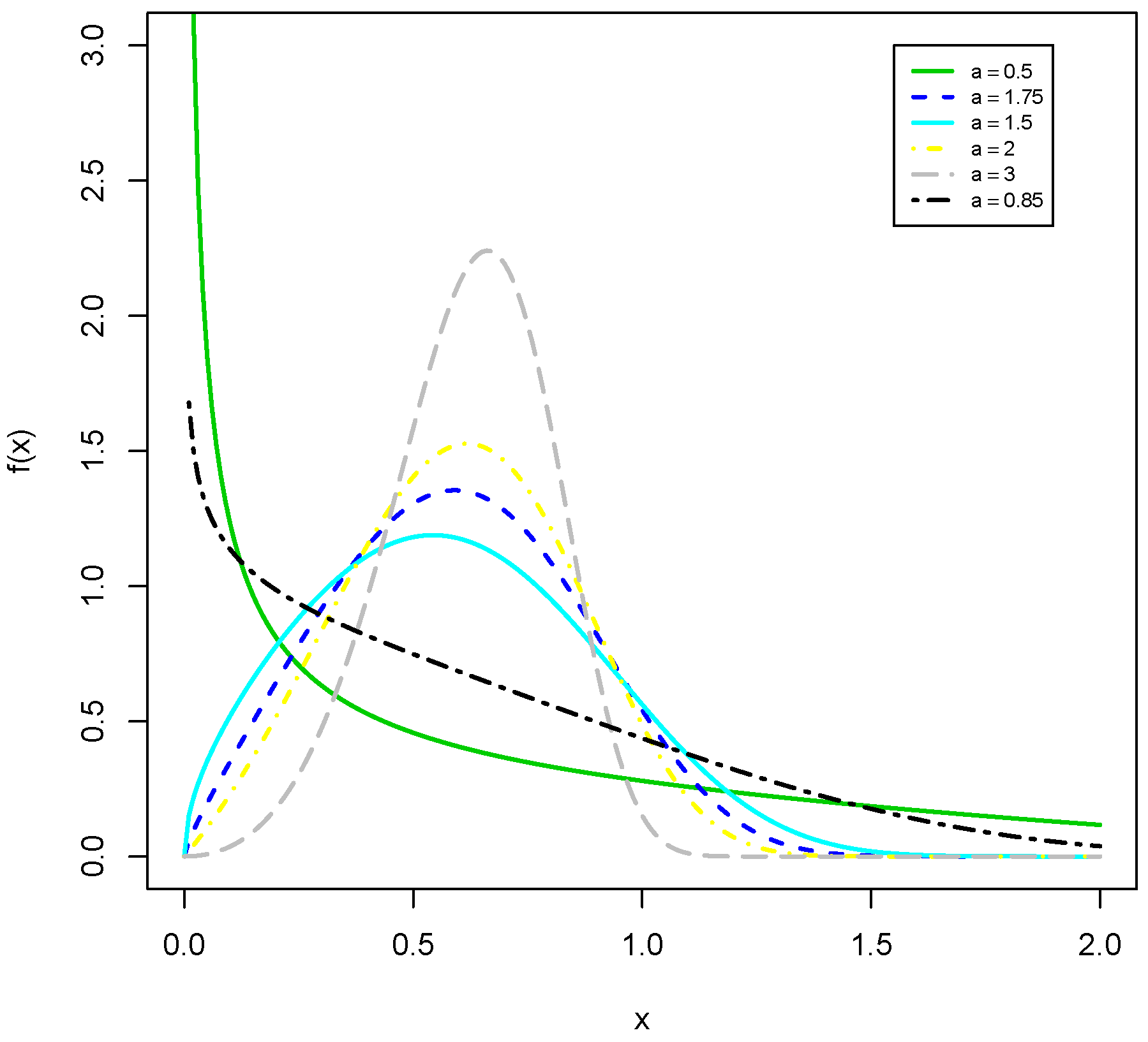
Remark 1.
Using (4) and the generalized binomial expansion, the MKiEx density reduces to
f x = m = 0 υ m g x ; m + 1 λ ,
where g x ; m + 1 λ is the PDF of the Ex distribution with scale parameter m + 1 λ , and
υ m = υ m j , k = j , k = 0 a 1 j + m j ! m + 1 j + 1 a + k k j + 1 a + k 1 m .
Equation (13) means that the MKiEx density can be expressed as a linear mixture of Ex densities. Hence, the properties of the MKiEx distribution can be obtained simply from those of the Ex distribution.
Figure 1 and 
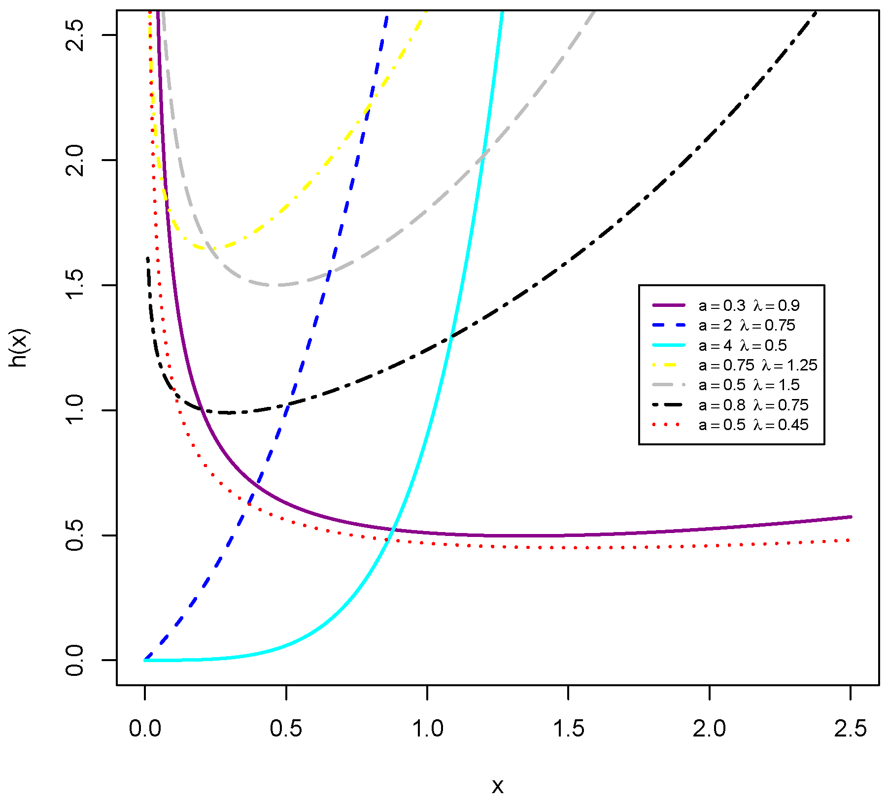
Figure 2 display some plots of the PDF and HR function, respectively, of the MKiEx distribution for selected values of a and λ . The plots of Figure 2 indicate that the HR function of the MKiEx model can be increasing, decreasing and bathtub shaped. One of the advantages of the MKiEx distribution over the exponential distribution is that the the last one cannot model phenomenon showing increasing, decreasing and bathtub failure rate shapes and therefore it becomes more flexible for analyzing lifetime data.
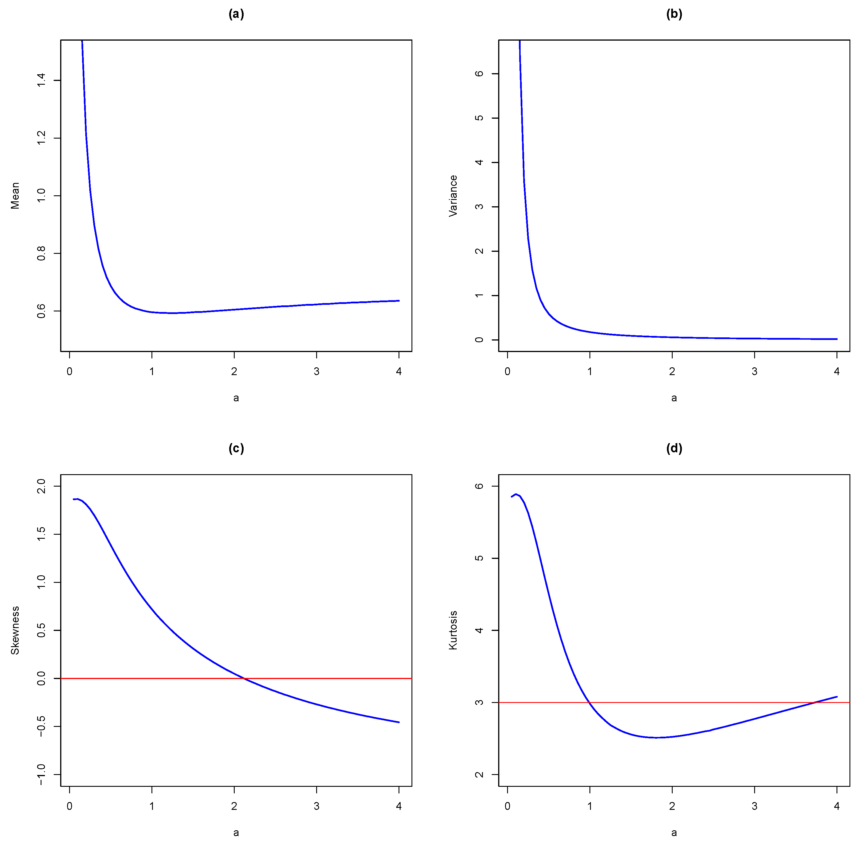
Remark 2.
The rth ordinary and incomplete moments of the MKiEx follows from (13) as
μ r = m = 0 inf υ m r ! m + 1 λ r and φ r ( t ) = m = 0 inf υ m γ ( 1 + r , m + 1 λ t ) m + 1 λ r .
The skewness and kurtosis measures can be evaluated from the ordinary moments using well-known relationships. Figure 3 presents the mean, variance, skewness and kurtosis of the MKiEx as a function in the shape parameter a with λ = 1 . Figure 3 shows that the mean is an increasing then decreasing then increasing function in the shape parameter a, while the variance is an increasing then decreasing function in a. Figure 3 indicates that the MKiEx is a flexible distribution. It can be symmetric, right skewed and left skewed. Moreover, it can be mesokurtic, platykurtic and leptokurtic. From Figure 3c,d, it is observed that for small values of a, the skewness and kurtosis increase then decrease as a increases.

4. Some Mathematical Properties for the HR Function of the MKiEx Distribution

The HR function of the MKiEx distribution given via Equation (11) discloses that for small values of x (i.e., x 0 + ), we have that
h ( x ) [ 1 exp ( λ x ) ] a 1 ,
and hence it is a decreasing function in x provided that a < 1 . On the other hand, we have that for large values of x (i.e., x ),
h ( x ) a λ exp ( a λ x ) ,
and so it is a growing function in x. Therefore, the MKiEx distribution is useful in modeling aging HR or bathtub-shaped HR. It is worth mentioning that most lifetime distributions with bathtub-shaped HR have some problems related to increasing number of parameters, algebraic complexity, and estimation problems. Interestingly, the MKiEx distribution has a bathtub-shaped HR that based on only two parameters.
Proposition 1.
The HR function of MKiEx distribution is an increasing function for a 1 and is a bathtub-shaped for a < 1 .
Proof. 
The first derivative of h ( x ) is
h ( x ) = a λ 2 exp ( a λ x ) ( 1 exp ( λ x ) ) a 2 a exp ( λ x ) .
Clearly, if a 1 , it then follows that h ( x ) > 0 for all x and thus h ( x ) is an increasing function in x . Now suppose that a < 1 , then h ( x ) = 0 if and only if
x = x 0 = ln ( a ) λ .
Therefore, h ( x ) < 0 if and only if x < x 0 and h ( x ) > 0 if and only if x > x 0 . This implies that h ( x ) has a minimum value at x = x 0 , which completes the proof.  ☐

5. Asymptotic Distributions of Order Statistics of the MKiEx Distribution

Order statistics are widely used in many different fields of statistical theory and applications. Suppose that X 1 , , X n are, independent and identically distributed random variables from the MKiEx distribution. The PDF of the ith order statistic, say X i , for i = 1 , , n , is given by
f X i x = l , k = 0 η l , k λ e λ x 1 e λ x l + 1 a + k 1 ,
where
η l , k = m = 0 j = 0 n i 1 j + m + l a m + 1 l l ! B i , n i + 1 n i j j + i 1 m l + 1 a + k k .
Certainly, extreme statistics such as M n = max ( X 1 , , X n ) and m n = min ( X 1 , , X n ) are members of the class of order statistics. The PDF of these extreme statistics are usually do not possess a closed form distribution (as in our case) and, therefore, asymptotics to their distributions are demanding because their applications are wide spread in many interesting areas. The following proposition provides the asymptotics distributions for the first and largest order statistic functions.
Proposition 2.
Let X 1 , , X n be a random sample from MKiEx distribution. We have
(i) 
The asymptotic distribution of the largest order statistics belongs to the domain of attraction for maxima of Gumbel type, i.e.,
lim x Pr ( a n ( M n b n ) < x ) = exp [ exp ( x ) ] ,
where a n > 0 and b n are normalizing constants.
(ii) 
The asymptotic distribution of the smallest order statistics belongs to the domain of attraction for minima of Weibull type, i.e.,
lim x Pr ( c n ( m n d n ) < x ) = 1 exp [ x a ] ,
where c n > 0 and d n are normalizing constants.
Proof. 
(i) Since F 1 ( 1 ) = , so we need to check whether the von Mises condition for the maximum domain of attraction of the Gumbel distribution are satisfied or not, see for example Embrechts et al. ([11], Equation (3.25), p. 140) or Theorem (8.3.3) (iii) of Arnold et al. [12]. Specifically, we need to show that
lim x d d x 1 h ( x ) = 0 ,
or equivalently, we have to show that
lim x S ( x ) F ( x ) f 2 ( x ) = 1 .
Since f ( x ) = h ( x ) S ( x ) , it then follows that
F ( x ) = h ( x ) S ( x ) + S ( x ) h ( x ) ,
where
h ( x ) = λ h ( x ) a exp ( λ x ) 1 exp ( λ x ) .
On substituting these quantities into Equation (15), we have
S ( x ) F ( x ) f 2 ( x ) = 1 + h ( x ) h 2 ( x ) = 1 + a exp ( λ x ) a 1 exp ( λ x ) a exp ( a λ x ) .
Clearly the second term in Equation (16) goes to 0, as x , and hence the result follows. The normalizing constants can be chosen using Theorem (8.3.4) (iii) of [12]. Additionally, since the von Mises condition is satisfied for the current problem, it follows Theorem (8.3.4) (iii) of [12] that a n = [ n f ( b n ) ] 1 and b n = F 1 ( 1 n 1 ) . For (ii), observe that for sufficiently small values of x ( x 0 + ), we have that F ( x ) 1 exp ( ( λ x ) a ) ) . Since F 1 ( 0 + ) = 0 < and
lim t 0 + F ( x t ) / F ( t ) = x a ,
it follows from Theorem (8.3.6) (ii) in [12] that the limiting distribution is G ˜ ( x ) = 1 exp ( x a ) , where the normalized constants can be calculated from Theorem (8.3.6) (ii) of [12] by taking d n = F 1 ( 0 + ) = 0 and c n = F 1 ( 1 / n ) .  ☐

6. Mean Residual Life

There is an additional important reliability measure which assess the mean remaining life expectancy of a component(individual) last to the time t. This measure is referred to as the mean residual life (MRL) function. The usefulness of the ML function lies in characterizing the entire residual failure time behind the time t contrary to the HR function which describes the failure in a small interval beyond t.
Mathematically speaking, the MRL function for a random variable X at time t is determined as the expected value of the conditional random variable of X t | X > t as given below
μ ( t ) = E ( X t | X > t ) = 0 S ( x + t ) S ( t ) d x = 1 S ( t ) t S ( x ) d x .
Observe that μ ( 0 ) = E ( X ) . It is observed that there is an interesting relation between HR function and MRL function as given below
h ( t ) = μ ( t ) μ ( t ) + 1 μ ( t ) ,
where μ ( t ) is the first derivative of μ ( t ) . Note that Equation (18) can be obtained by differentiating Equation (17) with respect to t . Apparently, Equation (18) indicates that the lifetime distribution can be uniquely defined using μ ( t ) and h ( t ) functions. Further, the inverse of the MRL and HR function are approximately equivalent when
lim t d ln ( μ ( t ) d t = 0 .
Explicit and approximate expressions for μ ( t ) are given in the following section.

6.1. MRL of the MKiEx Distribution

The first incomplete moments of the MKiEx model is
φ 1 ( t ) = m = 0 υ m γ ( 2 , m + 1 λ t ) m + 1 λ .
The MRL of X is defined by
μ t = 1 φ 1 t / S ( t ) t ,
where φ 1 t is given by (19) and S ( t ) = 1 F x is the survival function of the MKiEx distribution.
The MRL of X follows, by inserting φ 1 ( t ) in (20), as
μ t = 1 S ( t ) m = 0 υ m γ ( 2 , m + 1 λ t ) m + 1 λ t .
The computation of μ ( t ) via Equation (21) is unattractive. Alternatively, we provide an asymptotic tractable approximation to μ ( t ) for sufficiently large value of t ( t ). We have the following proposition.
Proposition 3.
For sufficiently large value of t , i.e., as t , we have that
μ ( t ) exp ( a λ t ) a λ .
Proof. 
We have that
μ ( t ) = 0 S ( x + t ) S ( t ) d x = 0 exp exp ( λ ( x + t ) 1 a exp exp ( λ t 1 a d x = 0 exp exp ( λ t ) 1 a exp ( λ ( x + t ) 1 a d x = 0 exp r ( x ; t ) d x ,
where r ( x ; t ) = exp ( λ t ) 1 a exp ( λ ( x + t ) 1 a . As t , we have that r ( x ; t ) exp ( a λ t ) 1 exp ( a λ x ) . Since exp ( a λ x ) 1 a λ x for small x ( x 0 + ), it then follows that
μ ( t ) 0 1 exp a λ exp ( a λ t ) x d x + 1 exp exp ( a λ t ) exp ( a λ x ) 1 d x .
On substituting u = exp ( a λ x ) 1 and letting c ( t ) = exp ( a λ t ) and k = exp ( a λ ) 1 , Equation (23) becomes
μ ( t ) = 1 exp a λ c ( t ) a λ c ( t ) + 1 a λ k exp c ( t ) u u + 1 d u = d ( t ) a λ c ( t ) + 1 a λ I ( t ) ,
where d ( t ) = 1 exp a λ c ( t ) and I ( t ) = k exp c ( t ) u u + 1 d u . Observe that
I ( t ) 1 k k inf exp c ( t ) u d u = 1 k exp ( k c ( t ) ) c ( t ) ,
and c ( t ) inf for large values of t , ( t ) . Accordingly,
0 lim t inf I ( t ) 1 k lim t exp ( k c ( t ) ) c ( t ) 0 , as t .
Since lim t d ( t ) = 1 , it then follows that d ( t ) / a λ c ( t ) a 1 λ 1 exp ( a λ t ) as t . Consequently, we have that μ ( t ) a 1 λ 1 exp ( a λ t ) .  ☐
Table 1 reports some values for the MRL function using asymptotic approximation in (22) as well as numerical integration for different choices of the parameters a and λ and several time points. It is noted that the two approximation methods are close and consistent when the time point increases; that is, the values obtained from Equation (22) become near of the values computed from numerical integration.
A useful approximation for the mean of the MKiEx distribution is μ = μ ( 0 ) 1 / ( a λ ) , where a is a shape parameter. The mean of the MKiEx distribution is determined by λ . This can be extended to be a log-linear regression model by making λ i = exp ( θ z i ) , where θ = ( θ 1 , , θ p ) is a parameter vector of length p and z i = ( z i 1 , , z i p ) is the vector of covariates or risk factors, i = 1 , , n . Specifically, the log-linear model can be written as
log ( E ( Y i | z i ) ) = α + ξ z i , i = 1 , , n ,
where E is the expectation operator, Y is the MKiEx random variable, α = log ( a ) , and ξ = θ . This would allow a variety of useful analyses, including a conventional nonlinear regression analysis. While the current paper aims to study the current distribution in terms of mathematical and statistical properties, we will consider the class of log-linear models relating to the proposed distribution in a future article.

6.2. MRL Shapes and Changing Points

In spite of MKiEx distribution has increasing or bathtub-shaped HR, we only focus on studying the changing points of the bathtub-shaped HR. Several researchers have discussed the connection between the HR and MRL functions. For instance, Gupta and Akman [13,14] proved that if a component has bathtub-shaped HR function, then its matching MRL function is upside-down bathtub, given that h ( 0 + ) . Mi [15] has proved that for the bathtub-shaped failure rate with a single inflection point 0 t * < , the MRL function has a unimodal shaped with a single turning point μ * such that μ * t * ; that is, the changing point of the MRL of a bathtub-shaped lifetime distribution go a head of that of the HR. For details on general results between the relation of MRL and HR functions, the reader is referred to Tang et al. [16]. We have the following proposition.
Proposition 4.
Let X MKi-G(a,λ) with a < 1 . The MRL of X has the upside-down bathtub shape.
Proof. 
Since for a , λ > 0 and x > 0 , we have that 1 + a λ x exp ( a λ x ) . Therefore, it follows that
μ r = r 0 x r 1 S ( x ) d x = r 0 x r 1 exp exp ( λ x ) 1 a d x r 0 exp ( λ x ) a d x , = r a 0 u r a 1 exp ( λ a u ) d u = r Γ ( r a ) a λ r < inf ,
where the last equality followed on using integration by substitution along with the gamma function. Since μ ( 0 + ) = μ 1 ( a λ ) 1 Γ ( a 1 ) < inf and h ( 0 + ) = inf ( a < 1 ), it then follows that h ( 0 + ) 1 / μ ( 0 + ) and, therefore, the result holds. ☐
We have the following proposition.
Proposition 5.
The asymptotic behaviors of the HR function and the reciprocal of the MRL are equivalent as t inf , i.e.,
lim t h ( t ) = lim t 1 μ ( t ) .
Proof. 
If we prove that
lim t d ln ( μ ( t ) d t = 0 ,
then we are finished. Observe that
d ln ( μ ( t ) d t = μ ( t ) μ ( t ) = h ( t ) 1 μ ( t ) .
Upon using Equation (22) as t , we have that h ( t ) = ( a λ ) 1 exp ( a λ t ) = 1 / μ ( t ) and, hence, the result follows. ☐
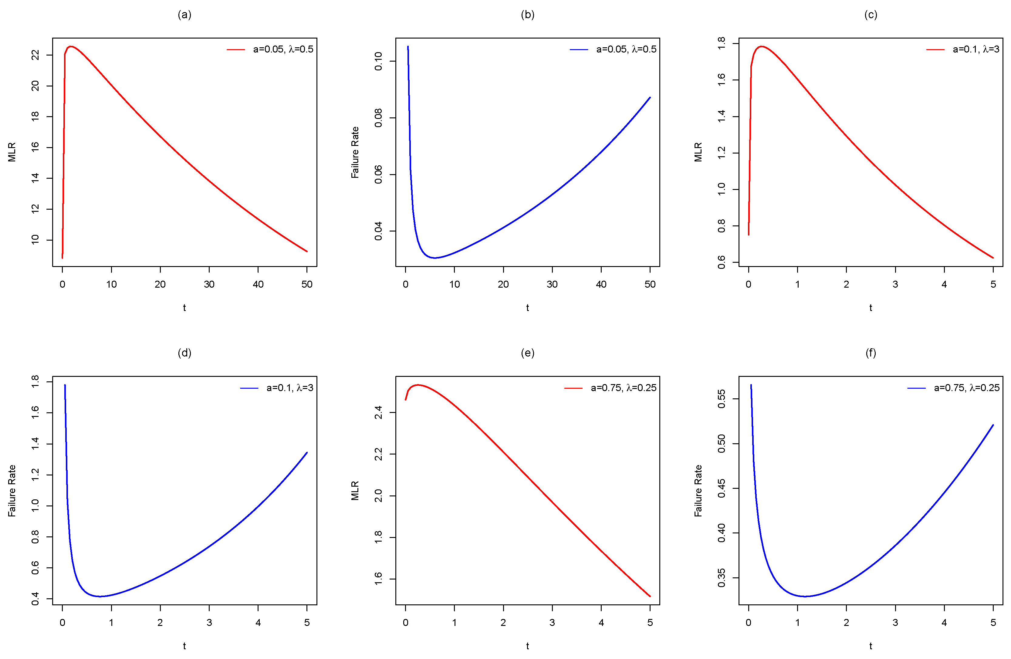
Here, we illustrate the relation between the MRL and HR functions for the Mkies distribution by using diagrams of the MRL and HR functions simultaneously. Figure 4b exhibits that the HR function has a bathtub-shaped with a unique turning point, that occurs at t * = 6.06 . The the matching style of the MRL is given in Figure 4a, which demonstrates a unimodal shaped. The diagram signifies that the changing point of the MRL μ * = 1.52 take place before that of the HR. The HR function given in Figure 4d shows the bathtub-shaped with inflection point happen at t * = 0.75 and, again, the matching MRL inflection point is μ * = 0.25 , which occurs before t * = 0.75 , Figure 4c Similarly, the HR in Figure 4f exhibits a bathtub-shaped HR with the inflection point of the HR occurs at t * = 1.16 , whereas the inflection point of the corresponding MRL given in Figure 4e occurs at μ * = 0.3 .

7. Parameters Estimation and Simulations

This section is devoted to investigate the maximum likelihood estimators (MLEs) of the parameters under complete and type-II censored samples. The approximate confidence intervals for the unknown parameters are also derived from the Fisher information matrix from complete and type-II censored samples. Furthermore, a simulation study is performed to study the behavior of the estimates.

7.1. Maximum Likelihood Estimation under Complete Sample

Let x 1 , , x n be a random sample of size n from the PDF in (3), then the log-likelihood function is given by
1 ( Θ ) = n log ( a λ ) + a λ i = 1 n x i i = 1 n ( e λ x i 1 ) a + ( a 1 ) i = 1 n log ( 1 e λ x i ) ,
where Θ = ( a , λ ) . The MLEs of a and λ can be obtained by solving the following two non-linear equations
1 ( Θ ) a = n a + λ i = 1 n x i i = 1 n ( e λ x i 1 ) a log ( e λ x i 1 ) + i = 1 n log ( 1 e λ x i ) = 0
and
1 ( Θ ) λ = n λ + a i = 1 n x i a i = 1 n x i e λ x i ( e λ x i 1 ) a 1 + ( a 1 ) i = 1 n x i ( e λ x i 1 ) 1 = 0 .
It is to be noted that Equations (24) and (25) cannot be solved explicitly, therefore, a numerical techniques can be used to obtain the MLEs of a and λ denoted by a ^ and λ ^ .
Using large sample approximation, the joint distribution of a ^ and λ ^ is asymptotically normally distributed with mean Θ and covariance matrix I 1 ( Θ ) . Practically, we use I 1 ( Θ ^ ) to estimate I 1 ( Θ ) , where I ( Θ ^ ) is the observed information matrix and
I 1 ( Θ ^ ) = 2 1 ( Θ ) a 2 2 1 ( Θ ) a λ 2 1 ( Θ ) λ a 2 1 ( Θ ) λ 2 1 | ( a , λ ) = ( a ^ , λ ^ ) = v a r ( a ^ ) c o v ( a ^ , λ ^ ) c o v ( λ ^ , a ^ ) v a r ( λ ^ ) ,
where
2 1 ( Θ ) a 2 = n a 2 i = 1 n ( e λ x i 1 ) a log 2 ( e λ x i 1 ) ,
2 1 ( Θ ) λ 2 = n λ 2 a i = 1 n x i 2 e λ x i ( e λ x i 1 ) a 1 [ ( a 1 ) ( 1 e λ x i ) 1 + 1 ] ( a 1 ) i = 1 n x i 2 ( e λ x i 1 ) 2 e λ x i
and
2 1 ( Θ ) a λ = i = 1 n x i i = 1 n x i e λ x i ( e λ x i 1 ) a 1 [ 1 + a log ( e λ x i 1 ) ] + i = 1 n x i ( e λ x i 1 ) 1 .
Now, the 100 ( 1 τ ) % approximate confidence intervals of the parameters a and λ can be obtained as
a ^ ± z τ / 2 v a r ( a ^ )
and
λ ^ ± z τ / 2 v a r ( λ ^ ) ,
where z τ / 2 is the upper ( τ / 2 ) th percentile of the standard normal distribution.

7.2. Maximum Likelihood Estimation under Type-II Censored Sample

Let x 1 , , x n be a random sample of size n, in type-II censoring scheme we observe only the first r order statistics. In this case, the likelihood function takes the form
L ( Θ ) = C i = 1 r f ( x i : r : n ) [ 1 F ( x r : r : n ) ] n r , x 1 : r : n x 2 : r : n x r : r : n ,
where C is a constant does not depend on the parameters and x 1 : r : n , x 2 : r : n , , x r : r : n is the censored data. From (26), the log-likelihood function without the constant term can be written as follows
2 ( Θ ) = r log ( a λ ) + a λ i = 1 r x i i = 1 r ( e λ x i 1 ) a + ( a 1 ) i = 1 r log ( 1 e λ x i ) ( n r ) ( e λ x r 1 ) a ,
where x i = x i : r : n , i = 1 , 2 , , r , for simplicity of notation and x r is the time of the r t h failure. Similarly, the MLEs of a and λ are the solution of the following two equations
2 ( Θ ) a = r a + λ i = 1 r x i i = 1 r ( e λ x i 1 ) a log ( e λ x i 1 ) + i = 1 r log ( 1 e λ x i ) ( n r ) ( e λ x r 1 ) a log ( e λ x r 1 ) = 0
and
2 ( Θ ) λ = r λ + a i = 1 r x i a i = 1 r x i e λ x i ( e λ x i 1 ) a 1 + ( a 1 ) i = 1 r x i ( e λ x i 1 ) 1 a ( n r ) x r e λ x r ( e λ x r 1 ) a 1 = 0 .
Again Equations (27) and (28) cannot be solved explicitly and a numerical techniques is needed to obtain the MLEs of a and λ . To obtain the approximate confidence intervals as mentioned in the previous subsection, the elements of the observed information matrix can be obtained as follow
2 2 ( Θ ) a 2 = r a 2 i = 1 r ( e λ x i 1 ) a log 2 ( e λ x i 1 ) ( n r ) ( e λ x r 1 ) a log 2 ( e λ x r 1 ) ,
2 2 ( Θ ) λ 2 = r λ 2 a i = 1 r x i 2 e λ x i ( e λ x i 1 ) a 1 [ 1 + ( a 1 ) ( 1 e λ x i ) 1 ] ( a 1 ) i = 1 r x i 2 e λ x i ( e λ x i 1 ) 2 a ( n r ) x r 2 e λ x r ( e λ x r 1 ) a 1 [ 1 + ( a 1 ) ( 1 e λ x r ) 1 ]
and
2 2 ( Θ ) a λ = i = 1 r x i i = 1 r x i e λ x i ( e λ x i 1 ) a 1 [ 1 + a log ( e λ x i 1 ) ] + i = 1 r x i ( e λ x i 1 ) 1 ( n r ) x r e λ x r ( e λ x r 1 ) a 1 [ 1 + a log ( e λ x r 1 ) ] .
Now, the same approach in the previous subsection is used to derive the approximate 100 ( 1 τ ) % confidence intervals of the parameters a and λ .

7.3. Simulation Results

In this subsection a simulation study is conducted to evaluate the performance of the MLEs of the parameters a and λ of the MKiEx distribution in terms of their mean square errors (MSEs) and confidence interval length (CIL) under complete and type-II censored samples. Equation (12) is used to generate the MKiEx variates. We consider the values 20 , 40 , 60 , 100 , 200 and 300 for n and the values of r are chosen to be 75 % of n. We choose different values for the parameters a and λ , we consider a = ( 0.5 , 1.5 , 2.5 , 5 ) and λ = ( 0.5 , 2.5 , 5 ) and replicate the process 1000 times. In each setting we obtain the average values (AVs) of the estimates and the corresponding MSEs, where
A V = k = 1 1000 θ ^ m , k 1000 and M S E = k = 1 1000 ( θ ^ m , k θ m ) 2 1000 , m = 1 , 2 , 3 and θ = ( a , λ ) .
We are also obtain the CIL and the corresponding coverage probabilities of the parameters a and λ . These results are displayed in Table 2, Table 3 and Table 4.
From Table 2, Table 3 and Table 4, it is observed that the MSEs decrease as the sample size increases in all the cases under the complete sample. Furthermore, the AVs of estimates tend to the true parameter values as the sample size increase. Furthermore, in the case of type-II censored sample as the number of failures r increases the MSEs decrease in all the cases as well as the estimates tend to the true values of the parameters. These results indicate that the MLEs of the parameters a and λ under the two schemes are asymptotically unbiased and consistent. As expected, the estimates under complete sample perform better than those under type-II sample in terms of MSEs. Moreover, the CIL decrease as the sample increases under the two schemes in all the cases. Furthermore, the CIL in the case of complete sample are smaller than those under type-II censored sample. This is because the complete sample has the larger number of observations. The simulation results show that the MKiEx distribution has a good results and very flexible to use in life testing experiment and one may use another types of censoring schemes.

8. Data Analysis

In this section, the MKiEx distribution is fitted to two real data sets and compared with other some competitive models. The fitted distributions are compared using some goodness-of-fit measures such as A I C (Akaike information), C A I C (consistent Akaike information), B I C (Bayesian information), and H Q I C (Hannan-Quinn information) criterions. We also consider the maximized log-likelihood under the model ( 2 ^ ) along with W * (Cramér-von Mises) and A * (Anderson-Darling) statistics.
The first data set is reported by Murthy et al. [17], and it represents failure times for a particular windshield device (84 observations). These data were studied by Afify et al. [18]. The second data set is reported by Xu et al. [19], and it contains 40 observations about time-to-failure (10 3 h ) of turbocharger of one type of engine. These data were studied by Afify et al. [20] and Cordeior et al. [21].
The new MKiEx model is compared with some competing models, such as the Marshall-Olkin exponential (MOEx) (Marshall and Olkin, [22]), Weibull (W), APEx, Kumaraswamy exponential (KEx), gamma (Ga), beta exponential (BEx) (Nadarajah and Kotz, [23]), exponentiated exponential (EEx) (Gupta and Kundu, [24]) and Ex distributions, whose PDFs (for x > 0 ) are:
MOEx : f ( x ) = α λ 1 1 α exp ( λ x ) 2 exp ( λ x ) , α , λ > 0 .
W : f ( x ) = β λ β x β 1 exp λ x β , β , λ > 0 .
APEx : f ( x ) = log α λ α 1 α 1 exp ( λ x ) exp ( λ x ) , α > 0 , α 1 , λ > 0 .
KEx : f ( x ) = a b λ exp ( λ x ) 1 exp ( λ x ) a 1 1 1 exp ( λ x ) a b 1 , a , b , λ > 0 .
Ga : f ( x ) = b a Γ a x a 1 exp x / b , a , b > 0 .
BEx : f ( x ) = λ B ( a , b ) 1 exp ( λ x ) a 1 exp ( b λ x ) , a , b , λ > 0 .
EEx : f ( x ) = α λ 1 exp ( λ x ) α 1 exp ( λ x ) , α , λ > 0 .
Table 5 and Table 6 report the numerical values of analytical measures for the competing distributions to both analyzed data sets. The maximum likelihood estimates and associated standard errors of the parameters are listed in Table 7 and Table 8.
In Table 5 and 
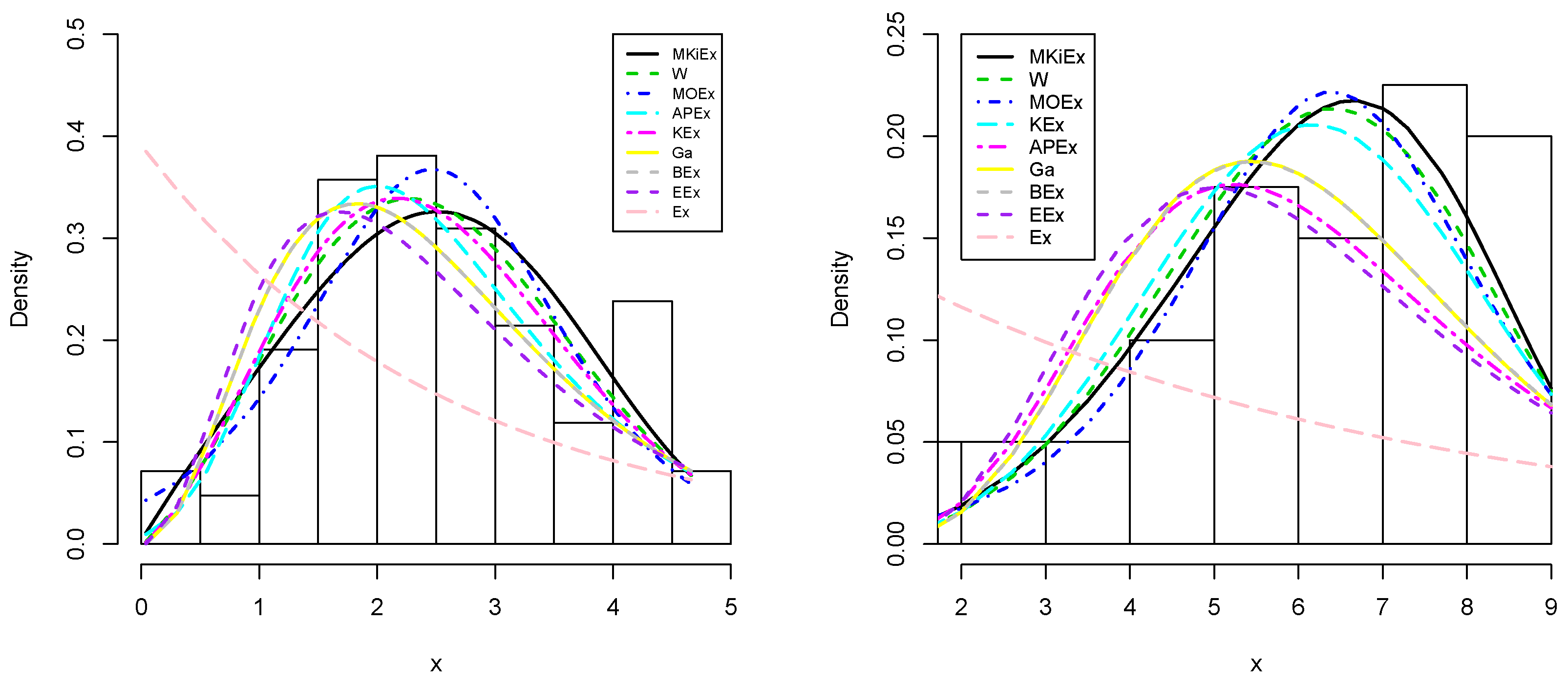
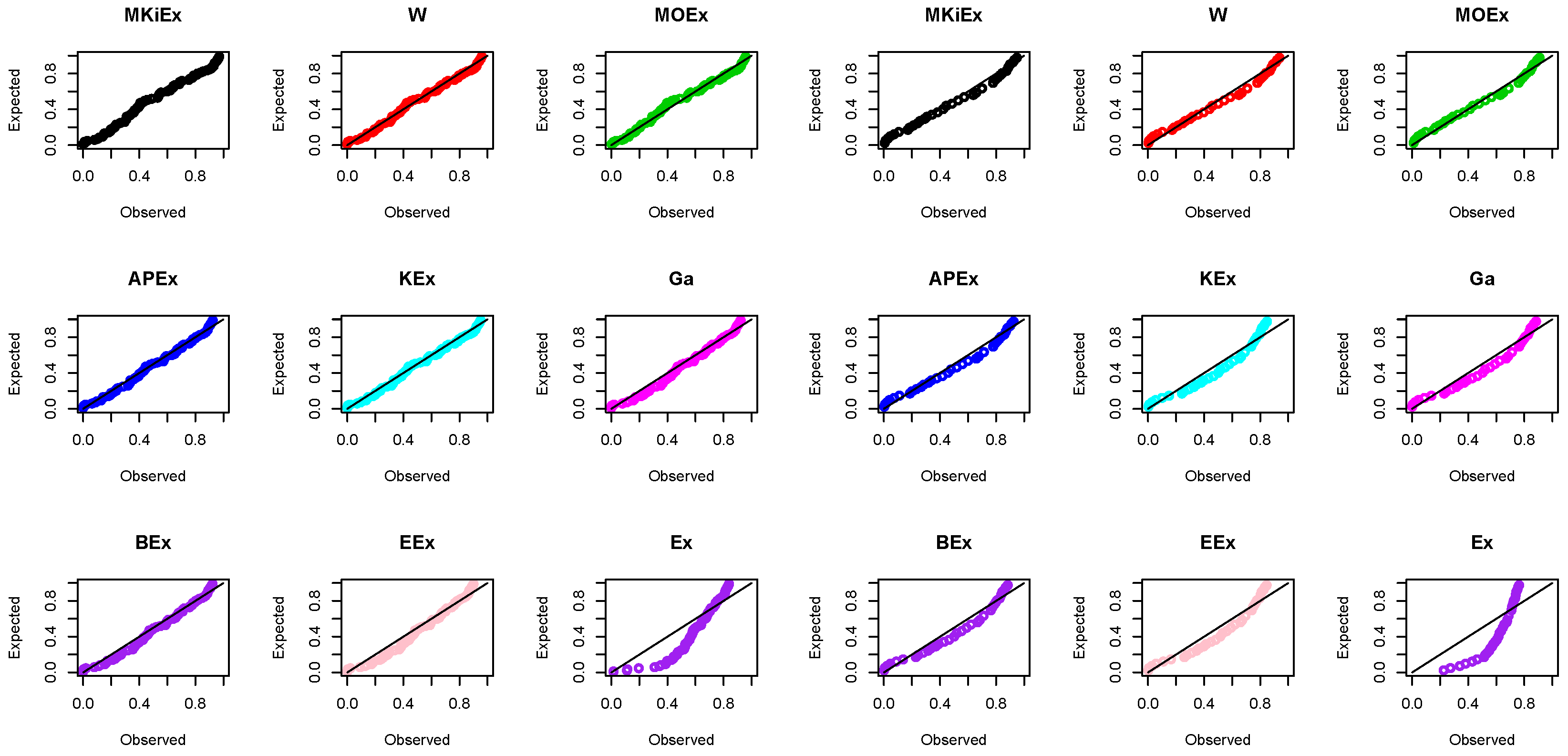
Table 6, we compare the fits of the MKiEx distribution with the W, MOEx APEx, KEx, Ga, BEx, EEx and Ex models. The values in Table 5 and Table 6 illustrate that the MKiEx distribution has close fit for both data sets, among the competing models. The histogram of the two data sets and the fitted MKiEx PDF are displayed in Figure 5. Further, the PP plots of the first and second data sets are displayed in Figure 6.

9. Conclusions

In this paper, we have introduced a new family of distributions called the the modified Kies family of distributions. Some mathematical properties of the proposed family are derived. We introduced a new two-parameter distribution by taking the the exponential distribution as baseline for the modified Kies family. The new distribution is called modified Kies exponential distribution. The modified Kies exponential distribution has one scale and one shape parameters. Its density function can take different shapes based on its shape parameter. Furthermore, the modified Kies exponential distribution failure rate function can be monotonically increasing, decreasing and bathtub shaped. The shape behavior of the hazard rate function and the Mean residual life are also discussed. We considered the maximum likelihood methods to estimate the parameters based on complete and type-II censored samples. An extensive simulation study is conducted to compare the performance of the estimates under the two schemes. The simulation results reveal that the maximum likelihood under the two schemes are asymptotically unbiased and consistent. Two real data analyses show that the modified Kies exponential distribution performs better than other distributions. This analysis proved that the modified Kies exponential distribution can be used effectively to model both positive and negative skewed data sets which are considered in the paper.

Author Contributions

A.A.A.-B., M.K.S., M.N., and A.Z.A. contributed equally to this work. All authors have read and agreed to the published version of the manuscript.

Funding

This project is supported by Researchers Supporting Project number (RSP-2020/156) King Saud University, Riyadh, Saudi Arabia.

Acknowledgments

The authors would like to thank the Editorial Board and two reviewers for their constructive comments that greatly improved the final version of the paper. This work was supported by King Saud University (KSU). The first author, therefore, gratefully acknowledges the KSU for technical and financial support.

Conflicts of Interest

The authors declare no conflict of interest.

References

  1. Kumar, C.S.; Dharmaja, S.H.S. On reduced Kies distribution. In Collection of Recent Statistical Methods and Applications; Kumar, C.S., Chacko, M., Sathar, E.I.A., Eds.; Department of Statistics, University of Kerala Publishers: Trivandrum, India, 2013; pp. 111–123. [Google Scholar]
  2. Kumar, C.S.; Dharmaja, S.H.S. The exponentiated reduced Kies distribution: Properties and applications. Commun. Stat. Theory Methods 2017, 46, 8778–8790. [Google Scholar] [CrossRef]
  3. Dey, S.; Nassar, M.; Kumar, D. Moments and estimation of reduced Kies distribution based on progressive type-II right censored order statistics. Hacet. J. Math. Stat. 2019, 48, 332–350. [Google Scholar] [CrossRef] [Green Version]
  4. Alzaatreh, A.; Lee, C.; Famoye, F. A new method for generating families of continuous distributions. Metron 2013, 71, 63–79. [Google Scholar] [CrossRef] [Green Version]
  5. Mahdavi, A.; Kundu, D. A new method for generating distributions with an application to exponential distribution. Commun. Stat. Theory Methods 2017, 46, 6543–6557. [Google Scholar] [CrossRef]
  6. Afify, A.Z.; Suzuki, A.K.; Zhang, C.; Nassar, M. On three-parameter exponential distribution: Properties, Bayesian and non-Bayesian estimation based on complete and censored samples. Commun. Stat. Simul. Comput. 2019. [Google Scholar] [CrossRef]
  7. Afify, A.Z.; Mohamed, O.A. A new three-parameter exponential distribution with variable shapes for the hazard rate: Estimation and applications. Mathematics 2020, 8, 135. [Google Scholar] [CrossRef] [Green Version]
  8. Lemonte, A.J.; Barreto-Souza, W.; Cordeiro, G.M. The exponentiated Kumaraswamy distribution and its log-transform. Braz. J. Probab. Stat. 2013, 27, 31–53. [Google Scholar] [CrossRef]
  9. Lorenz, M.O. Methods of measuring the concentration of wealth. Publ. Am. Stat. Assoc. 1905, 9, 209–219. [Google Scholar] [CrossRef]
  10. Bonferroni, C.E. Elementi di Statistica Generale; Seeber: Firenze, Italy, 1930. [Google Scholar]
  11. Embrechts, P.; Kluppelberg, C.; Mikosch, T. Modelling Extremal Events for Insurance and Finance; Springer: Berlin/Heidelberg, Germany, 1997. [Google Scholar]
  12. Arnold, B.C.; Balakrishnan, N.; Nagaraja, H.N. First Course in Order Statistics; John Wiley: New York, NY, USA, 1992. [Google Scholar]
  13. Gupta, R.C.; Akman, H.O. Mean residual life functions for certain types of non-monotonic ageing. Commun. Stat. Stoch. Models 1995, 11, 219–225. [Google Scholar]
  14. Gupta, R.C.; Akman, H.O. Erratum: Mean residual life functions for certain types of non-monotonic ageing. Commun. Stat. Stoch. Models 1995, 11, 561–562. [Google Scholar]
  15. Mi, J. Bathtub failure rate and upside-down bathtub mean residual life. IEEE Trans. Reliab. 1995, 44, 388–391. [Google Scholar] [CrossRef]
  16. Tang, L.C.; Lu, Y.; Chew, E.P. Mean residual life of lifetime distributions. IEEE Trans. Reliab. 1999, 48, 73–78. [Google Scholar] [CrossRef]
  17. Murthy, D.N.P.; Xie, M.; Jiang, R. Weibull Models; Wiley: Hoboken, NJ, USA, 2004. [Google Scholar]
  18. Afify, A.Z.; Cordeiro, G.M.; Yousof, H.M.; Alzaatreh, A.; Nofal, Z.M. The Kumaraswamy transmuted-G family of distributions: Properties and applications. J. Data Sci. 2016, 14, 245–270. [Google Scholar]
  19. Xu, K.; Xie, M.; Tang, L.C.; Ho, S.L. Application of neural networks in forecasting engine systems reliability. Appl. Soft Comput. 2003, 2, 255–268. [Google Scholar] [CrossRef]
  20. Afify, A.Z.; Altun, E.; Alizadeh, M.; Ozel, G.; Hamedani, G.G. The odd exponentiated half-logistic-G family: Properties, characterizations and applications. Chil. J. Stat. 2017, 8, 65–91. [Google Scholar]
  21. Cordeiro, G.M.; Afify, A.Z.; Ortega, E.M.; Suzuki, A.K.; Mead, M.E. The odd Lomax generator of distributions: Properties, estimation and applications. J. Comput. Appl. Math. 2019, 347, 222–237. [Google Scholar] [CrossRef]
  22. Marshall, A.W.; Olkin, I. A new method for adding a parameter to a family of distributions with application to the exponential and Weibull families. Biometrika 1997, 84, 641–652. [Google Scholar] [CrossRef]
  23. Nadarajah, S.; Kotz, S. The beta exponential distribution. Reliab. Eng. Syst. Saf. 2006, 91, 689–697. [Google Scholar] [CrossRef]
  24. Gupta, R.D.; Kundu, D. Generalized exponential distribution: Different method of estimations. J. Stat. Comput. Simul. 2001, 69, 315–337. [Google Scholar] [CrossRef]
Figure 1. Plots of the MKiEx PDF with λ = 1 and different values of a.
Mathematics 08 01345 g001
Figure 2. Plots of the MKiEx HR function with λ = 1 and different values of a.
Mathematics 08 01345 g002
Figure 3. Plots of (a) Mean, (b) variance, (c) skewness and (d) kurtosis of MKiEx distribution as a function of a and for λ = 1 .
Mathematics 08 01345 g003
Figure 4. Plots of MRL and HR functions along with their changing points: (a) μ * = ( 1.52 , 22.56 ) ; (b) t * = ( 6.06 , 0.03 ) ; (c) μ * = ( 0.25 , 1.78 ) ; (d) t * = ( 0.75 , 0.42 ) ; (e) μ * = ( 0.3 , 2.53 ) ; (f) t * = ( 1.16 , 0.33 ) .
Mathematics 08 01345 g004
Figure 5. Fitted densities for data I (left) and data II (right).
Mathematics 08 01345 g005
Figure 6. PP plots for data I (left) and data II (right).
Mathematics 08 01345 g006
Table 1. MRL for some parameter values.
( λ , a )tEquation (21) Equation (22)
( 0.5 , 0.5 ) 0.51.7328 3.5300
11.7029 3.1152
31.3031 1.8895
50.9025 1.1460
( 0.5 , 2 ) 0.50.7833 0.6065
10.4875 0.3679
30.0600 0.0498
50.0073 0.0067
( 2 , 0.5 ) 0.50.3802 0.6065
10.2731 0.3679
30.0475 0.0498
50.0067 0.0067
( 2 , 2 ) 0.50.0436 0.0338
10.0052 0.0046
30.0000 0.0000
50.0000 0.0000
Table 2. The AVs of estimates and corresponding MSEs (in parentheses) in the first row and the CIL and corresponding coverage probability (in parentheses) in the second row.
ParametersComplete SampleType-II Censored Sample
λ a λ a λ a
n = 20 , r = 15
0.50.50.5414 (0.0295)0.5415 (0.0184)0.5921 (0.0703)0.5619 (0.0252)
0.5541 (92.000)0.4490 (95.000)0.7742 (93.900)0.5079 (95.100)
2.50.5064 (0.0013)2.6781 (0.3152)0.5107 (0.0017)2.7869 (0.5744)
0.1296 (92.300)1.9173 (94.900)0.1413 (89.800)2.4719 (95.600)
50.5022 (0.0003)5.3863 (1.2185)0.5039 (0.0004)5.5717 (2.1836)
0.0642 (92.200)3.7935 (95.500)0.0697 (91.800)4.9314 (95.700)
2.50.52.6949 (0.6558)0.5372 (0.0163)2.9613 (1.6375)0.5591 (0.0225)
2.7653 (94.500)0.4457 (95.900)3.8570 (93.700)0.5053 (96.600)
2.52.5174 (0.0298)2.6801 (0.3074)2.5405 (0.0407)2.8037 (0.5939)
0.6441 (92.800)1.9180 (95.300)0.7001 (90.700)2.4872 (95.800)
52.5087 (0.0075)5.3876 (1.3604)2.5178 (0.0097)5.5798 (2.2017)
0.3222 (93.500)3.7944 (93.700)0.3488 (90.700)4.9485 (94.300)
50.55.3826 (2.2964)0.5395 (0.0169)5.8447 (6.4747)0.5598 (0.0254)
5.5062 (92.700)0.4492 (94.100)7.5949 (92.900)0.5066 (94.800)
2.55.0256 (0.1147)2.6812 (0.2855)5.0609 (0.1516)2.7823 (0.5399)
1.2801 (93.200)1.9225 (96.100)1.3989 (91.200)2.4669 (95.400)
55.0168 (0.0301)5.4014 (1.3143)5.0297 (0.0368)5.5681 (2.2238)
0.6405 (92.600)3.8080 (94.400)0.6982 (90.800)4.9366 (95.000)
n = 40, r = 30
0.50.50.5232 (0.0116)0.5170 (0.0072)0.5477 (0.0266)0.5274 (0.0098)
0.3804 (93.700)0.3046 (94.200)0.5174 (94.600)0.3369 (94.500)
2.50.5025 (0.0006)2.6062 (0.1276)0.5045 (0.0008)2.6569 (0.2204)
0.0915 (93.300)1.3157 (95.500)0.1005 (93.000)1.6654 (96.400)
50.5010 (0.0001)5.1950 (0.4652)0.5016 (0.0002)5.2585 (0.8101)
0.0460 (93.900)2.5789 (95.600)0.0505 (93.000)3.2946 (96.400)
2.50.52.6279 (0.3048)0.5139 (0.0070)2.7359 (0.6370)0.5234 (0.0092)
1.9189 (94.400)0.3033 (94.000)2.6024 (93.600)0.3344 (93.400)
2.52.5104 (0.0142)2.5840 (0.1272)2.5187 (0.0187)2.6161 (0.1838)
0.4611 (95.500)1.3070 (95.500)0.5083 (94.000)1.6399 (96.100)
52.5054 (0.0035)5.1348 (0.4378)2.5120 (0.0043)5.2660 (0.8327)
0.2329 (94.600)2.5423 (96.100)0.2528 (93.200)3.2983 (95.700)
50.55.1425 (1.0370)0.5230 (0.0068)5.3810 (2.2305)0.5339 (0.0096)
3.7066 (92.700)0.3074 (95.300)5.0082 (92.900)0.3407 (96.000)
2.55.0159 (0.0564)2.6100 (0.1350)5.0410 (0.0750)2.6684 (0.2216)
0.9128 (94.000)1.3171 (94.500)0.9996 (92.800)1.6730 (94.600)
55.0078 (0.0143)5.1640 (0.4642)5.0169 (0.0185)5.2713 (0.8868)
0.4630 (93.700)2.5571 (95.100)0.5052 (92.100)3.2997 (94.700)
Table 3. The AVs of estimates and corresponding MSEs (in parentheses) in the first row and the CIL and corresponding coverage probability (in parentheses) in the second row.
ParametersComplete SampleType- Censored Sample
λ a λ a λ a
n = 60 , r = 45
0.50.50.5129 (0.0067)0.5120 (0.0045)0.5323 (0.0145)0.5206 (0.0060)
0.3037 (94.300)0.2460 (95.100)0.4108 (94.300)0.2711 (94.100)
2.50.5010 (0.0004)2.5666 (0.0825)0.5026 (0.0005)2.6035 (0.1401)
0.0752 (94.800)1.0562 (93.500)0.0827 (94.600)1.3317 (94.100)
50.5006 (0.0001)5.1208 (0.2938)0.5011 (0.0001)5.1751 (0.4973)
0.0379 (94.800)2.0692 (96.300)0.0415 (93.900)2.6456 (95.900)
2.50.52.5511 (0.1602)0.5110 (0.0040)2.6234 (0.3520)0.5167 (0.0049)
1.5134 (93.400)0.2462 (95.400)2.0341 (92.900)0.2693 (94.900)
2.52.5065 (0.0097)2.5526 (0.0739)2.5148 (0.0118)2.5924 (0.1223)
0.3776 (93.700)1.0499 (95.800)0.4148 (94.100)1.3266 (95.200)
52.5011 (0.0024)5.1057 (0.2941)2.5039 (0.0029)5.1657 (0.5125)
0.1899 (94.700)2.0619 (95.300)0.2079 (94.400)2.6400 (95.000)
50.55.1999 (0.6874)0.5056 (0.0043)5.3485 (1.4232)0.5115 (0.0053)
3.1074 (95.500)0.2441 (93.500)4.1981 (94.600)0.2668 (94.500)
2.55.0028 (0.0373)2.5601 (0.0779)5.0159 (0.0461)2.5900 (0.1248)
0.7516 (94.700)1.0543 (95.000)0.8283 (94.600)1.3252 (95.6000)
55.0056 (0.0096)5.1044 (0.3008)5.0128 (0.0117)5.1703 (0.4920)
0.3802 (93.600)2.0615 (94.500)0.4157 (93.000)2.6432 (94.900)
n = 100, r = 75
0.50.50.5072 (0.0035)0.5047 (0.0023)0.5164 (0.0072)0.5084 (0.0027)
0.2335 (95.300)0.1885 (95.300)0.3128 (95.400)0.2052 (95.700)
2.50.4995 (0.0002)2.5484 (0.0438)0.5004 (0.0003)2.5713 (0.0739)
0.0581 (95.500)0.8116 (95.100)0.0640 (95.600)1.0192 (95.800)
50.5004 (0.0001)5.0596 (0.1714)0.5010 (0.0001)5.1219 (0.2896)
0.0296 (94.400)1.5784 (94.500)0.0323 (94.700)2.0275 (95.000)
2.50.52.5382 (0.0958)0.5058 (0.0024)2.5832 (0.1802)0.5095 (0.0029)
1.1676 (94.000)0.1888 (95.000)1.5638 (95.100)0.2055 (94.800)
2.52.5056 (0.0057)2.5355 (0.0425)2.5119 (0.0071)2.5653 (0.0746)
0.2930 (94.700)0.8070 (96.600)0.3224 (94.600)1.0168 (94.900)
52.5020 (0.0015)5.0713 (0.1702)2.5043 (0.0018)5.1205 (0.2789)
0.1475 (94.500)1.5824 (94.900)0.1613 (93.200)2.0267 (96.500)
50.55.0905 (0.3954)0.5048 (0.0024)5.1742 (0.7711)0.5080 (0.0029)
2.3448 (94.600)0.1885 (94.600)3.1400 (93.600)0.2050 (94.500)
2.55.0001 (0.0226)2.5260 (0.0418)5.0100 (0.0287)2.5499 (0.0702)
0.5868 (94.500)0.8042 (95.300)0.6467 (93.200)1.0104 (96.000)
55.0044 (0.0056)5.0709 (0.1730)5.0090 (0.0073)5.1196 (0.2801)
0.2950 (94.200)1.5821 (94.400)0.3226 (94.100)2.0267 (95.700)
Table 4. The AVs of estimates and corresponding MSEs (in parentheses) in the first row and the CIL and corresponding coverage probability (in parentheses) in the second row.
ParametersComplete SampleType-II Censored Sample
λ a λ a λ a
n = 200 , r = 150
0.50.50.5021 (0.0018)0.5035 (0.0011)0.5063 (0.0033)0.5053 (0.0014)
0.1631 (94.400)0.1329 (96.200)0.2171 (94.900)0.1441 (95.900)
2.50.5009 (0.0001)2.5085 (0.0214)0.5012 (0.0001)2.5149 (0.0325)
0.0417 (95.200)0.5649 (95.400)0.0461 (95.400)0.7047 (95.500)
50.499 (0.00003)5.0218 (0.0778)0.500 (0.00004)5.0434 (0.1348)
0.0210 (94.400)1.1074 (95.700)0.0230 (94.700)1.4114 (95.300)
2.50.52.5184 (0.0424)0.5042 (0.0012)2.5449 (0.0804)0.5063 (0.0014)
0.8175 (95.100)0.1330 (95.300)1.0894 (95.200)0.1444 (94.700)
2.52.5006 (0.0029)2.5186 (0.0216)2.5014 (0.0036)2.5222 (0.0323)
0.2074 (94.100)0.5671 (94.600)0.2296 (93.800)0.7066 (96.100)
52.4992 (0.0007)5.0459 (0.0824)2.5000 (0.0008)5.0646 (0.1519)
0.1043 (95.300)1.1130 (94.500)0.1146 (95.400)1.4174 (93.800)
50.55.0349 (0.1784)0.5046 (0.0012)5.0851 (0.3217)0.5067 (0.0015)
1.6336 (94.800)0.1331 (95.500)2.1758 (95.200)0.1445 (95.700)
2.55.0075 (0.0112)2.5060 (0.0196)5.0090 (0.0136)2.5084 (0.0311)
0.4173 (95.100)0.5646 (95.300)0.4623 (95.200)0.7026 (95.200)
55.0011 (0.0029)5.0461 (0.0860)5.0028 (0.0035)5.0628 (0.1351)
0.2088 (93.800)1.1131 (95.200)0.2293 (94.900)1.4169 (95.700)
n = 300, r = 225
0.50.50.5009 (0.0011)0.5042 (0.0008)0.5018 (0.0019)0.5047 (0.0009)
0.1327 (94.900)0.1087 (94.400)0.1756 (95.700)0.1175 (94.500)
2.50.5002 (0.0001)2.5119 (0.0140)0.5005 (0.0001)2.5201 (0.0223)
0.0339 (95.200)0.4613 (94.900)0.0375 (95.300)0.5764 (95.300)
50.501 (0.00002)5.0083 (0.0541)0.503 (0.00002)5.0406 (0.0979)
0.0172 (93.900)0.9024 (95.300)0.0188 (93.800)1.1518 (93.600)
2.50.52.5116 (0.0287)0.5027 (0.0008)2.5238 (0.0504)0.5037 (0.0009)
0.6662 (95.700)0.1084 (95.700)0.8849 (95.800)0.1173 (95.100)
2.52.5024 (0.0019)2.5078 (0.0143)2.5043 (0.0023)2.5152 (0.0217)
0.1700 (95.600)0.4608 (94.600)0.1879 (95.300)0.5754 (94.100)
52.4998 (0.0004)5.0359 (0.0559)2.5006 (0.0006)5.0517 (0.0906)
0.0853 (94.800)0.9064 (94.800)0.0936 (95.200)1.1543 (95.500)
50.55.0226 (0.1168)0.5016 (0.0008)5.0568 (0.2087)0.5031 (0.0010)
1.3335 (95.000)0.1081 (94.400)1.7751 (95.500)0.1172 (94.300)
2.55.0030 (0.0079)2.5114 (0.0156)5.0060 (0.0098)2.5171 (0.0240)
0.3394 (94.500)0.4615 (93.000)0.3755 (93.200)0.5758 (93.700)
55.0007 (0.0020)5.0225 (0.0568)5.0014 (0.0024)5.0306 (0.0879)
0.1711 (94.000)0.9043 (94.400)0.1880 (94.200)1.1494 (94.400)
Table 5. Numerical values of the analytical measures for data set I.
Model 2 ^ A IC CA IC HQ IC B IC W * A *
MKiEx255.772259.772259.920261.726264.6340.069720.56030
MOEx256.504260.504260.652262.458265.3660.066460.51737
W260.106264.106264.254266.061268.9680.060130.59718
APEx263.358267.358267.506269.3124272.2120.072990.72287
KEx262.442268.442268.742271.374275.7350.068120.68505
Ga273.874277.874278.022279.828282.7350.156551.33817
BEx273.889279.889280.189282.821287.1820.156691.33911
EEx279.681283.681283.829285.635288.5430.210631.69461
Ex325.754327.754327.803328.731330.1850.160881.36725
Table 6. Numerical values of the analytical measures for data set II.
Model 2 ^ A IC CA IC HQ IC B IC W * A *
MKiEx162.539166.539166.863167.760169.9160.053470.41127
W164.951168.951172.328170.172172.3280.076990.57304
MOEx167.205171.205171.529172.426174.5820.086010.61795
APEx177.984181.984182.308183.205185.3620.234111.52728
KEx167.025173.025173.6913174.857178.0910.102050.73648
Ga174.821178.821179.145180.042182.1980.205261.36163
BEx174.834180.834181.501182.666185.9010.205441.36264
EEx180.285184.285184.609185.507187.6630.275741.76008
Ex226.639228.639228.744229.249230.32740.206521.36890
Table 7. Parameter estimates and standard errors for data set I.
ModelEstimates (Standard Errors)
MKiEx (a, λ )1.7837 (0.1629)0.2367 (0.0107)
MOEx ( α , λ )35.1070 (15.1651)1.4285 (0.1494)
W ( λ , β )0.3492 (0.01677)2.3743 (0.2096)
APEx ( α , λ )841.2509 (954.4471)0.9522 (0.0791)
KEx (a,b, λ )2.5583 (0.2905)50.8582 (53.7323)0.0851 (0.0478)
Ga (a,b)3.4922 (0.5152)1.3655 (0.2166)
BEx (a,b, λ )3.4929 (0.5155)34.9964 (58.0101)0.0377 (0.0603)
EEx ( α , λ )3.5605 (0.6109)0.7579 (0.0769)
Ex ( λ )0.3910 (0.0427)
Table 8. Parameter estimates and standard errors for data set II.
ModelEstimates (Standard Errors)
MKiEx ( α , λ )2.9281 (0.3978)0.0994 (0.0040)
W ( λ , β )0.1445 (0.0061)3.8725 (0.5176)
MOEx ( α , λ )285.7258 (240.3562)0.8837 (0.1202)
APEx ( α , λ )211835.1 (11866.59)0.4791 (0.0310)
KEx (a,b, λ )4.4517 (0.8353)123.7773 (170.078)0.0602 (0.0317)
Ga (a,b)7.7227 (1.6909)1.2351 (0.2794)
BEx (a,b, λ )7.7268 (1.6926)54.6596 (56.1356)0.0213 (0.0203)
EEx ( α , λ )9.5142 (2.8959)0.4498 (0.0578)
Ex ( λ )0.1599 (0.0253)

