The Lambert-F Distributions Class: An Alternative Family for Positive Data Analysis


1
Departamento de Matemática, Facultad de Ciencias Básicas, Universidad de Antofagasta, Antofagasta 1240000, Chile
2
Instituto de Ciências Matemáticas e de Computação, Universidade de São Paulo, São Carlos 13560-095, SP, Brazil
*
Author to whom correspondence should be addressed.
Mathematics 2020, 8(9), 1398; https://0-doi-org.brum.beds.ac.uk/10.3390/math8091398
Submission received: 18 July 2020
/
Revised: 11 August 2020
/
Accepted: 17 August 2020
/
Published: 21 August 2020
(This article belongs to the Special Issue Probability, Statistics and Their Applications)
Abstract
:In this article, we introduce a new probability distribution generator called the Lambert-F generator. For any continuous baseline distribution F, with positive support, the corresponding Lambert-F version is generated by using the new generator. The result is a new class of distributions with one extra parameter that generalizes the baseline distribution and whose quantile function can be expressed in closed form in terms of the Lambert W function. The hazard rate function of a Lambert-F distribution corresponds to a modification of the baseline hazard rate function, greatly increasing or decreasing the baseline hazard rate for earlier times. Herein, we study the main structural properties of the new class of distributions. Special attention is given to two particular cases that can be understood as two-parameter extensions of the well-known exponential and Rayleigh distributions. We discuss parameter estimation for the proposed models considering the moments and maximum likelihood methods. Finally, two applications were developed to illustrate the usefulness of the proposed distributions in the analysis of data from different real settings.
1. Introduction
In recent years, towards more flexibility, many studies have been developed in which new methods are proposed to add one or more parameters to a baseline probability distribution. These methods have given way to the generation of models with more complex parametric structures and more flexibility in aspects such as the shapes of the density and hazard rate functions and the asymmetry or kurtosis of the distribution.
One of the most popular methods is to propose a new cumulative distribution function (cdf) considering a suitable transformation of the cdf of a certain random variable of interest. More specifically, if X is a random variable with cdf , then
where is a nondecreasing function such that as , and as , for , is a cdf.
Different analytical expressions for can be found in the literature. If , , then the cdf in Equation (1) corresponds to the cdf of the exponentiated distributions class; see Gupta et al. [1], Nadarajah and Kotz [2], Al-hussaini [3], Castillo et al. [4] and Gómez-Déniz et al. [5], among others. If , where and denotes the incomplete beta function ratio, then Equation (1) corresponds to the cdf of the beta-generated distributions class; see Eugene et al. [6], Jones [7], Jones [8] and Nadarajah and Kotz [9], among others. Similarly, other alternative expressions for can be found in Marshall and Olkin [10], Shaw and Buckley [11], Zografos and Balakrishnan [12], Cordeiro and de Castro [13], Lai [14] and Badr et al. [15], to name just a few.
In this paper, we propose a new distribution generator called the Lambert-F generator. The proposed generator is obtained from Equation (1) by considering a new analytical expression for the function given by , for and . The result is a new cdf with an extra shape parameter having the quantile function written in closed form in terms of the Lambert W function, hence the name of the generator. Note that a Lambert-F distribution is reduced to the baseline distribution when ; that is, the baseline distribution and the respective Lambert version are nested distributions. We will show that the hazard rate function (hrf) of a Lambert-F distribution corresponds to a modification of the baseline hrf, greatly increasing or decreasing the baseline hrf for the lower values of X (earlier times). This can be interpreted as a perturbation of the baseline hrf at earlier times.
The Lambert W function, which corresponds to the inverse function of , with z being any complex number, plays an important role in this work. This is a many-valued function satisfying , for every complex number . By restricting to be a real-valued function, the complex variable z is then replaced by the real variable x, and the function is defined only for to be double-valued in the interval and simple-valued (principal branch, denoted by ) for . More details of the Lambert W function can be found in Corless et al. [16] and Brito et al. [17]. Recently, Visser [18] showed that the Lambert W function can be used in the distribution of prime numbers.
In the statistical literature, Goerg [19] introduced new families of distributions using the Lambert W function in the context of random variable transformations. In our approach we apply a transformation to a baseline cdf, as can be seen in Definition 1.
We emphasize the fact that the Lambert-F generator can be used to extend any arbitrary probability distribution, regardless of whether it is the distribution of a discrete or continuous random variable and whether it has positive, real or bounded support. However, in this paper we consider the case in which the baseline distribution is a continuous distribution with positive support. Other cases might be the subject of future research.
The remainder of the paper is organized as follows. In Section 2, we propose the distributions generator. In Section 3, main structural properties of the generator are studied. In Section 4, two special models are derived with its main properties. Section 6 discusses parameter estimation using the moments and maximum likelihood methods. In Section 7, we describe a simulation study carried out to assess the performances of the estimators. In Section 8, two applications evidence that the proposed distributions may present a better fit than other models such as the Weibull and gamma distributions. The conclusions of this work are presented in Section 9. Computational code used in Section 6, Section 7 and Section 8 is available on request.
2. Lambert-F Distribution Generator
Definition 1.
A random variable X follows a Lambert-F distribution, denoted as , if its cdf is given by
where is an extra parameter and is the cdf of a continuous and positive baseline random variable with parameter vector η.
Note that the function inherits the support of the baseline distribution and that when . We refer to the cdf presented in Equation (2) as the Lambert-F distribution generator. From now on, we will denote and to simplify the notation.
Proposition 1.
Let . Then, the probability density function (pdf), the survival function (sf) and the hazard rate function (hrf) of X are given, respectively, by
where , , and are the pdf, the cdf, thesf and the hrf of the baseline distribution, respectively.
Proof.
From the above results, we note that the extra parameter allows the pdf and the hrf of the Lambert-F distributions to present a wider range of shapes than those of the baseline distributions. These shapes are discussed in detail in the following section.
3. Properties
In this section, we study the pdf and hrf shapes of the Lambert-F distributions class, discuss the stochastic ordering of Lambert-F random variables and derive analytical expressions for the quantile function and the raw moments of the Lambert-F distributions class.
3.1. Shapes
The shapes of the pdf and the hrf presented in Corollary 1 can be described analytically. First of all, we see that: (i) ; (ii) and .
Secondly, under the assumption that and exist, the critical points of the pdf of X are the roots of the equation
A root of Equation (6) will be a local maximum, a local minimum or an inflection point in the cases , or , respectively, where
The critical points of the hrf of X are the roots of the equation
A root of Equation (7) will be a local maximum, a local minimum or an inflection point in the cases , or , respectively, where
While giving even greater attention to the hrf of the Lambert-F distributions, we point out the following:
- The hrf of the Lambert-F distribution approximates the hrf of the baseline distribution F when x is large enough, that is, as .
- The hrf of the Lambert-F distribution is greater than the hrf of the baseline distribution F if and only if .
- If and the hrf of the baseline distribution F is a nondecreasing monotonic function, then the hrf of the Lambert-F distribution is a nondecreasing monotonic function.
In view of the above, the application of the proposed Lambert transformation to a baseline distribution has a simple justification in terms of the hrf of the resulting model. The hrf induced by the Lambert-F generator is more distant from the baseline hrf for lower values of X (earlier times), as can be seen in Figure 1 and Figure 2.
It should be taken into account that Equations (6) and (7) allow a detailed description of the shapes of the pdf and the hrf of a Lambert-F distribution once the definition functions of the baseline distribution are specified. The non-existence or existence of one or more solutions for these equations will depend jointly on the performance of the parameter and on the analytical structure of the specified baseline distribution.
3.2. Stochastic Order
The ordering of continuous positive random variables is an important tool for judging comparative behavior. It is well known that a random variable X is smaller than a random variable Y in the stochastic order () if for all x, in the hazard rate order () if for all x and in the likelihood ratio order () if decreases in x. Additionally, the implications
are well known Shaked and Shanthikumar [20].
Proposition 2.
Let and . If , then and therefore and .
Proof.
First, notice that
is a nondecreasing function if and only if , where
Some calculations show that
Now, note that implies ; that is, is decreasing in x, which means . The remaining affirmations were derived from the implications in Equation (8). □
A direct consequence of Proposition 2 is that the hrf of the Lambert-F distribution is less than the hrf of the baseline F distribution when , which is consistent with the observation Equation (2) in Section 3.1.
3.3. Quantile Function
Proposition 3.
Let . Then, the quantile function of X is given by
where is the quantile function of the baseline distribution and is the principal branch of the Lambert W function.
Proof.
From Equation (2) it can be observed that the baseline cdf can be written as
Then, solving this equation with respect to x, we obtain the expression in Equation (9) for . In the special case , the result is obtained directly by calculating the inverse function of the baseline cdf. □
Remark 1.
For , we have that . Then, the Lambert W function has a unique solution (principal branch). For we have that . Then, the Lambert W function has two solutionsm but only the solution of the principal branch is admissible due to the condition of obtaining positive random values.
3.4. Moments
Proposition 4.
Let . Then, for the r-th raw moment of X can be written as
where denotes the quantile function of the baseline distribution.
Proof.
From the Lambert-F pdf in Corollary 1, we have that
and by applying the change of variable , the result is obtained. □
4. Two Special Cases
In what follows, two new two-parameter models generated from the results in Corollary 1 are introduced. The well-known exponential and Rayleigh distributions are taken as baseline distributions in the generation of these new models.
Lambert-exponential model. The random variable X follows the Lambert-exponential distribution with scale parameter , denoted as , if its pdf and hrf for are given, respectively, by
Lambert–Rayleigh model. The random variable X follows the Lambert–Rayleigh distribution with scale parameter , denoted as , if its pdf and hrf for are given, respectively, by
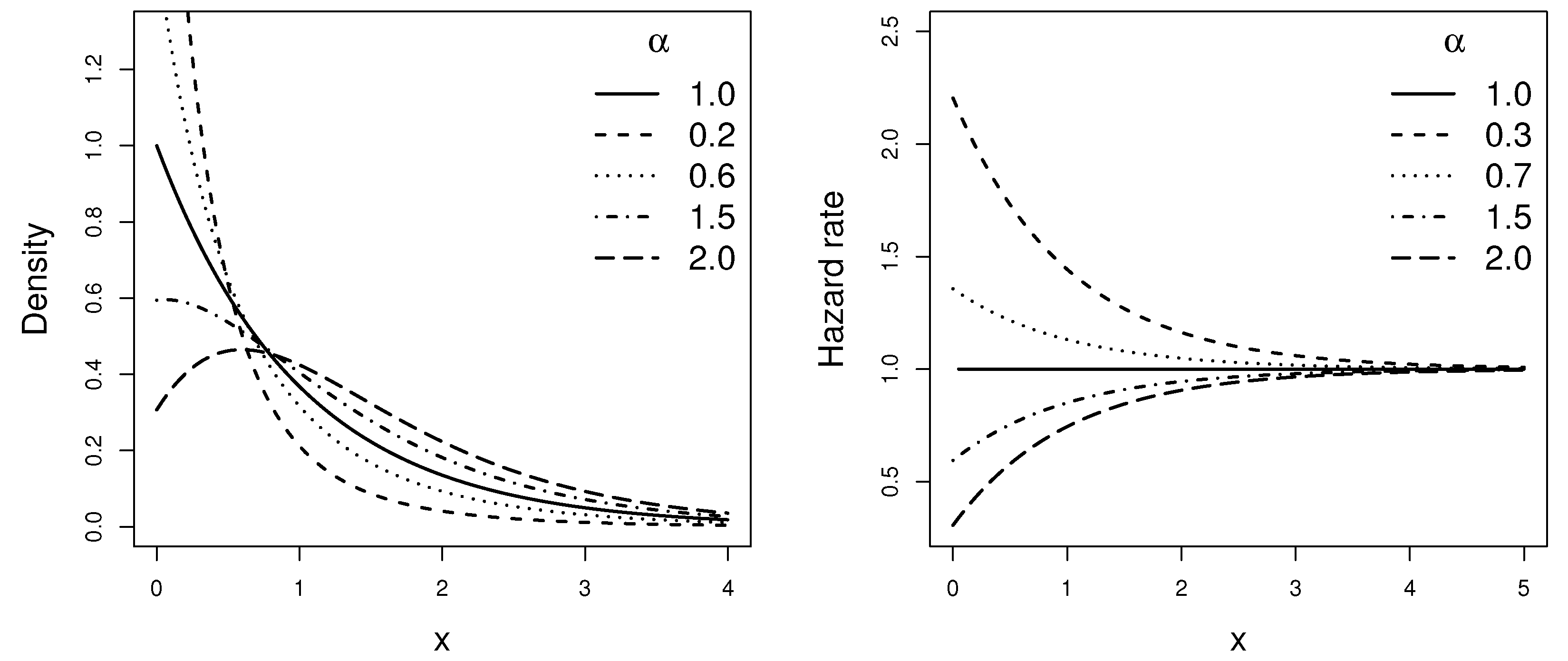
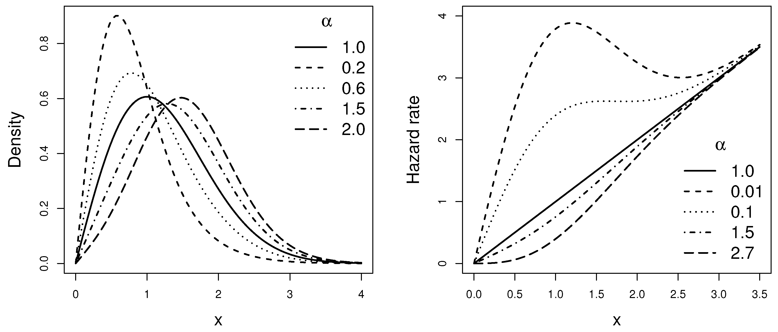
The new two-parameter distributions described above are members of the well-known and popular shape and scale distributions family. The scale in both models is inherited from the respective baseline distribution, while the shape parameter arises from the application of the Lambert transformation to the baseline distribution. Figure 1 and Figure 2 display some plots of the pdfs and the hrfs of the above models for and different values of shape parameter.
5. Characterizing the LE and LR Distributions
This section describes the main structural properties of the LE and LR distributions.
5.1. Description and Comparison of Shapes
From the results in Section 3.1, it is possible to analytically describe the shapes of the pdf and the hrf of the above models. In the sequel, the pdf and the hrf of the LE and LR models can be analytically described.
- Let . Then,
- (a)
- , and .
- (b)
- Considering , the pdf of X is a monotonically decreasing function when or , and it is a unimodal function for or . The mode of X is given by
- (c)
- The hrf of X is a monotonically decreasing function when , a monotonically increasing function when and a constant function for .
- Let . Then,
- (a)
- , and .
- (b)
- The pdf of X is a unimodal function for (Mode without explicit analytic expression).
- (c)
- The hrf of X is a monotonically increasing function when and presents the increasing–decreasing–increasing shape for . The local maximum and the local minimum are given by , , where and denote the principal and non-principal branches of the Lambert W function, respectively.
The shapes of the pdf and the hrf for the LE model are similar to those presented by other two-parameter models, such as Weibull (W) and gamma (G). It is important to note that the LE, W and G models are two-parameter extensions of the exponential model, so the comparison between these models is quite natural. A similar observation can be made for the LR and W models because both are two-parameter extensions of the Rayleigh model.
In Table 1 and Table 2, we present a comparison of the shapes of density and hazard rate functions of the LE and LR models with those of the W and G models. In Table 1, it is seen that the pdfs of the LE distribution presents similar shapes to those of the W and G models. However, unlike the W and G models, the pdf of the LE distribution tends to as when it is unimodal; that is, it tends to a positive finite value. This led us to establish that the LE distribution can properly fit datasets whose frequency distributions are unimodal while having observations lumped around 0. On the other hand, the pdf of the LR model presents only the unimodal shape but (as will be seen later) with variations of asymmetry and kurtosis. In Table 2, it is seen that the shapes presented by the hrf of the LE distribution are similar to those of the W and G distributions. However, from the results presented in Table 2, and similarly to the behavior of the LE pdf, an important difference can be observed in the behavior of the LE hrf for lower values of x (times close to 0). On the other hand, the LR distribution is the only distribution (among the distributions considered) that has a hrf that can present the increasing–decreasing–increasing shape.
5.2. Quantile Function, Moments and Related Quantities
In the following corollaries, derived from the results in Section 3, analytical expressions are presented for the quantile function, mean, variance, raw moments and asymmetry and kurtosis coefficients for the LE and LR distributions.
Corollary 1.
Let and . Then, for the quantile functions for and are given by
where
Corollary 2.
Let and . Then, for and , the r-th raw moment of is given by , where
such that , , and .
Corollary 3.
Let and . Then, for , the mean and the variance of are given by
respectively, where and , for and , are as in Corollary 2.
Corollary 4.
Let and . Then, the asymmetry () and kurtosis () coefficients for , with , are given by
where , for and , are as in Corollary 2.
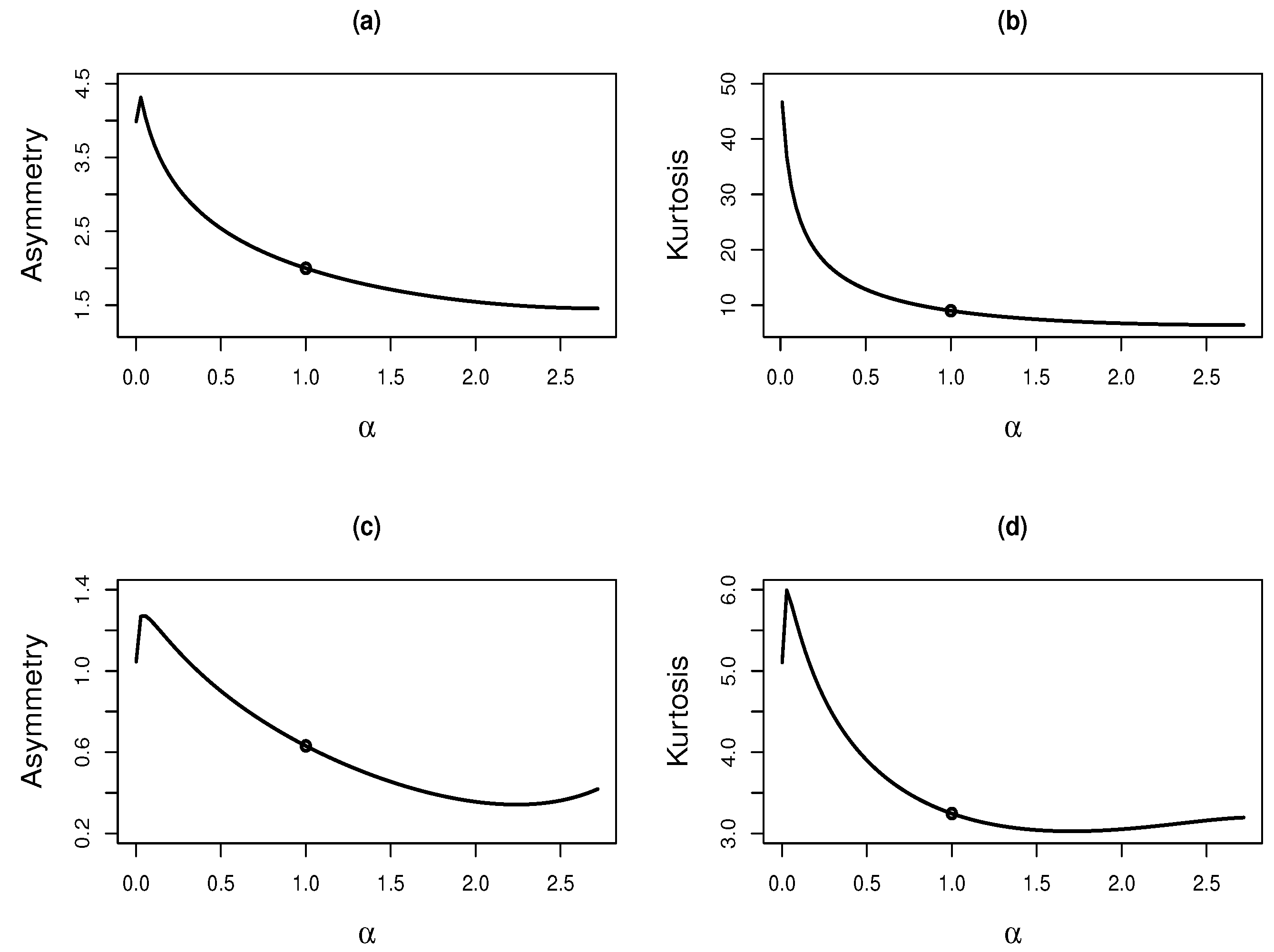
Figure 3 shows plots of the asymmetry and kurtosis coefficients for both the LE and LR distributions, and for the baseline distributions, exponential and Rayleigh, respectively. Note that the asymmetry and kurtosis values of the baseline distributions were extended to a range of values in the respective Lambert versions, showing greater flexibility of these latter distributions. The asymmetry and kurtosis ranges for the LE distribution were (1.456, 4.461) and (6.416, 48.814), respectively, and for the LR distribution (0.342, 1.274) and (3.027, 6.005), respectively. These ranges were calculated by minimizing and maximizing the asymmetry and kurtosis coefficients in Corollary 4. We used the integrate function of the R programming language R Core Team [21] to compute the functions. The optimize function was used to minimize and maximize the coefficients.
6. Parameter Estimation
In this section, we discuss parameter estimation for the Lambert-F distributions using the moments and maximum likelihood methods.
6.1. Moment Estimators
For a random sample of the random variable , the moment estimators are obtained by solving the equations generated by matching the first raw moments with the first sampling moments.
For a random sample of the random variable , for , such that and , the moment estimator for is given by the root of the equation
and the moment estimator for is given by
where , for and , are as in Corollary 2 and and are the first and second sampling moments, respectively, associated with the sample of the random variable .
Remark 2.
From Equation (11), it is seen that the moment estimators for α cannot be obtained in closed form. To obtain the moment estimate of this parameter, Equation (11) should be solved numerically. We solved Equation (11) using the uniroot function from the R programming language. Once obtained the estimate of α, we used this value to obtain the moment estimate for the σ parameter from Equation (12).
6.2. Maximum Likelihood Estimators
For a random sample of a random variable X with LE or LR distribution (given in Section 4), the log-likelihood function is given by
where , and are the baseline functions given in Table 3.
Since expressions of the ML estimators are not available in closed form, ML estimates are computed using the optim function in R via the L-BFGS-B method with the moments estimates, and , as the initial values for the iterative process.
Under regularity conditions, the asymptotic distribution of the ML estimator of is , where is the expected information matrix. Due to the analytical structure of Equation (13), it is not easy to obtain the analytical expression of this matrix. However, it can be approximated by minus the Hessian matrix evaluated at the ML estimate of the parameters. For the LE and LR models, the elements of the Hessian matrix are given by
with and for the LE and LR models as in Table 3.
In the case of survival data, under the consideration of non-informative right-censoring and assuming independence between failure times () and censoring times (), , the observed time for the i-th individual is given by with the respective failure indicator if or if . Thus, for a observed sample , the log-likelihood function for the LE and LR models is given by
where , and are as in the Table 3. For , , Equation (14) is reduced to Equation (13). Inference based on Equation (14) can be performed in a similar manner, as was done in the uncensored case, as described above. Finally, note that the above procedures can be extended to the case where the baseline distribution has k parameters.
7. Simulation Study
In this section, we present a simulation study done to assess the performances of the moments and maximum likelihood estimates for the parameters of the models in Section 4. We generated random samples of sizes from the LE and LR distributions, respectively, for different values of its parameters. The random numbers were generated by through the following steps:
- Generate ;
- Compute , for ;
- Compute , where is the baseline quantile function.
We used the W function of the LambertW package in R Goerg [22] to compute the principal branch of Lambert W function. Table 4 and Table 5 show averages, empirical standard deviations (SD), averages of asymptotic standard errors (SE) and roots of the simulated mean square errors (RMSE) of the estimates of and for the LE and LR distributions. Looking at Table 4, it can be seen that both the moments method and the ML method provide acceptable estimates of the parameters of the LE distribution. However, the ML method provides estimates with lower biases, and the SD and RMSE were smaller than those provided by the moments method. In addition, SD, SE and RMSE were closer for the ML method. The same held for SD and RMSE from the moments method. The estimators of the parameters of the LR distribution in Table 5 had similar behavior, with the exception that SD and RMSE were smaller for the moments method when the sample size was .
8. Application
In this section, we present two applications to real data using the Lambert-exponential (LE) and Lambert–Rayleigh (LR) distributions. With the first application, we provide evidence that the LR distribution may present a better fit than the Weibull (W), gamma (G), generalized Rayleigh (GR) Surles and Padgett [23] and Rayleigh (R) models. Similarly, with the second application we show that the LE distribution presents a better fit than the W, G, generalized exponential (GE) Gupta et al. [1] and exponential (E) models.
8.1. Nicotine Measurement Data
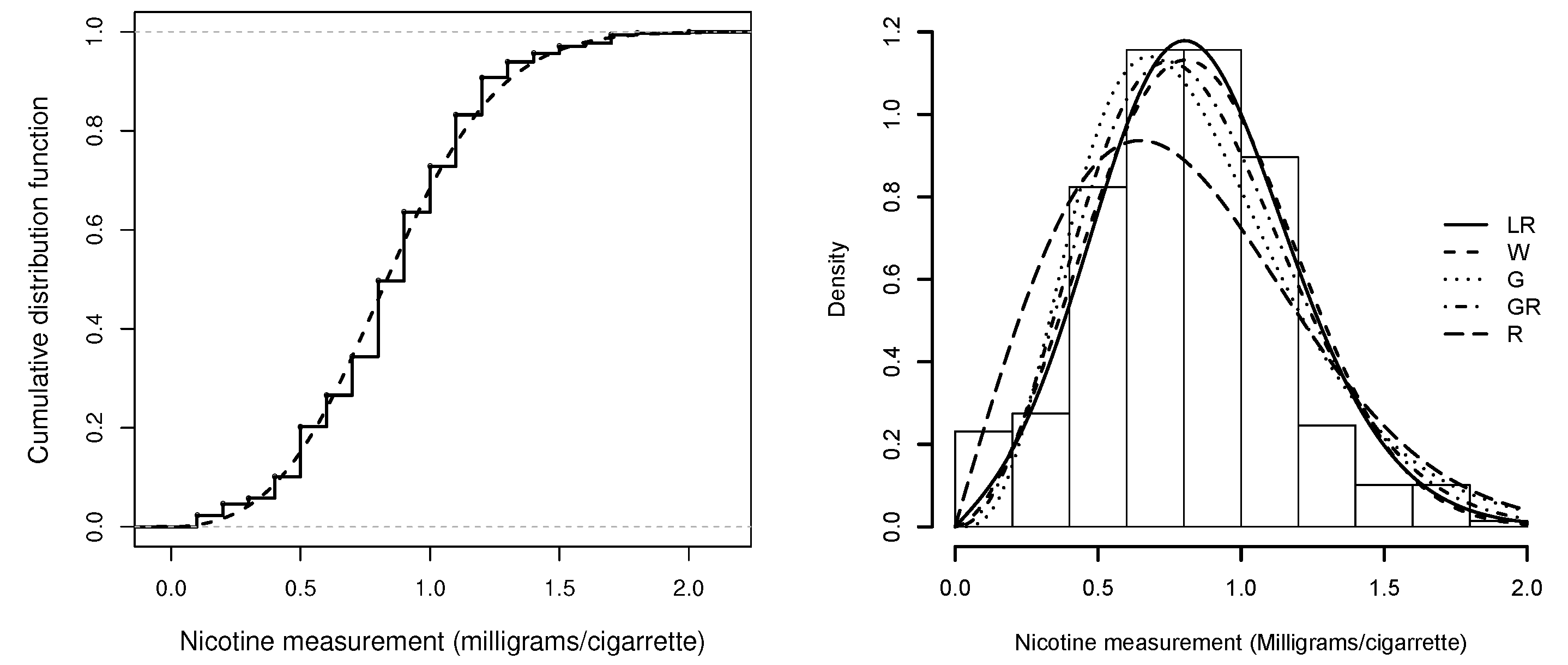
We considered a dataset of 346 nicotine measurements (milligrams per cigarette) collected in 1998 by the Federal Trade Commission (FTC), Washington, DC. For a recent analysis of this data, see Handique et al. [24]. Some descriptive statistics for these data are the following; average milligrams per cigarette, standard deviation milligrams per cigarette, sample asymmetry coefficient and sample kurtosis coefficient .
Using results from Section 6.1, moment estimates were computed, leading to the following values: and . Using the moment estimates as initial values, ML estimates were computed, and they are presented in Table 6 with the standard errors in parenthesis. For each fitted model, the maximum value of the log-likelihood function is also reported in Table 6. Note that the LR model has a maximum value of the log-likelihood function larger than the other models.
In order to compare the distributions, we computed the usual Akaike information criterion (AIC) Akaike [25] and Bayesian information criterion (BIC) [26]. Table 6 reports AIC and BIC values for each fitted model. We can see that AIC and BIC show a better fit for the LR model. In Figure 4 (left panel), the empirical cdf for nicotine measurements is compared with the cdf of the fitted LR model, and we can see that the two curves are close. In the same figure (right panel), the histograms for the nicotine measurement data and the fitted density functions are presented. Here, we see that the LR distribution fits nicotine measurement data better than the other distributions.
8.2. Monoclonal Gammopathy Data
This dataset comprises survival times (days) from diagnosis to the last follow-up of 241 subjects diagnosed with apparently benign monoclonal gammopathy at Mayo Clinic (US). Of the 241 subjects, 16 survived until the end of the follow-up and three had monoclonal gammopathy of undetermined significance (MGUS) detected on the day of death. This dataset was previously analyzed in Kyle [27] and is currently available under the name mgus in the survival package in R Therneau [28].
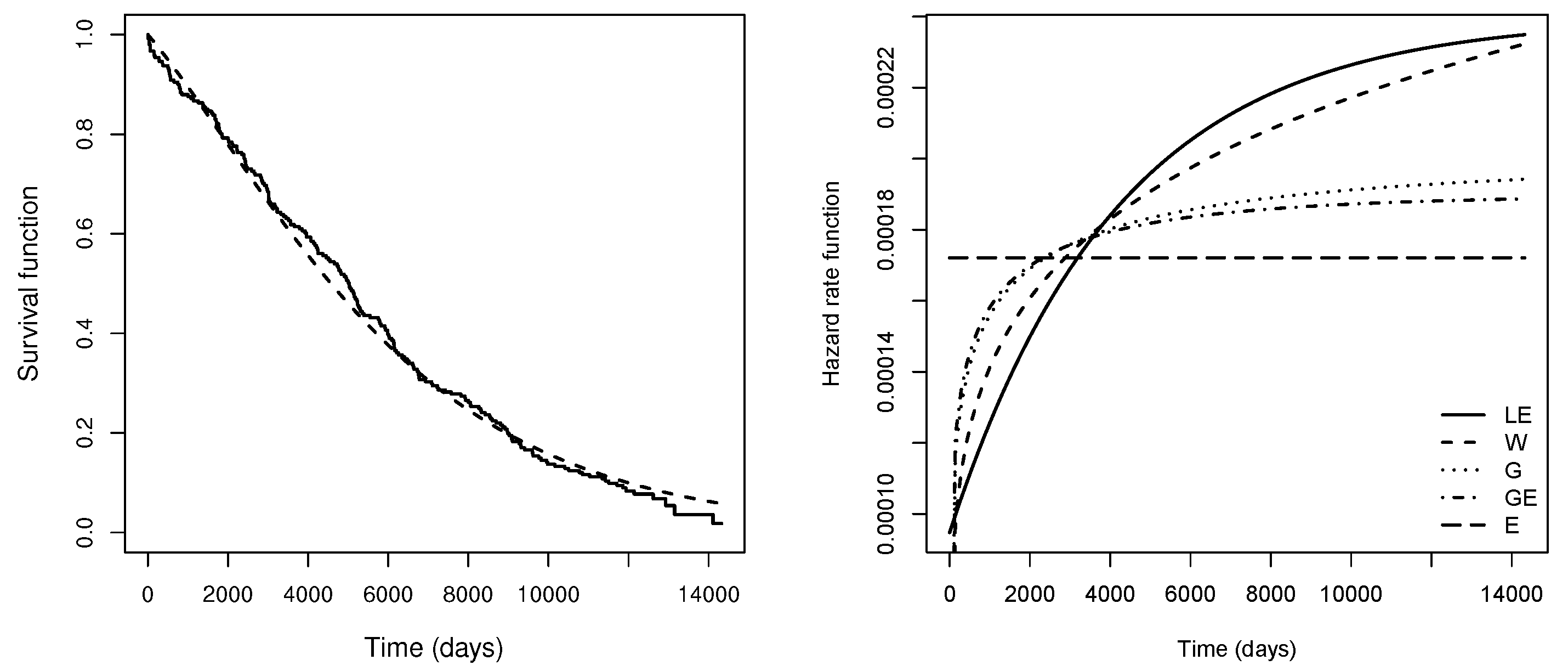
Maximum likelihood estimates, with standard errors in parentheses; the maximum values of the log-likelihood functions; and AIC and BIC values for the E, GE, G, W and LE models are reported in Table 7. It can be noted that AIC and BIC show better fit of the LE model. In Table 7, for the LE model the estimate of is so that the hazard rate function monotonically increases to reach a plateau at . In Figure 5 (left panel), the survival curves estimated by the fitted LE distribution and by the Kaplan–Meier estimator are close. In the right panel, the hazard rate function for each distribution fitted to the monoclonal gampathy data is presented. Here, we observe that the hazard rate of the LE distribution is lower than the hazard rates of the other distributions in the first 3600 days (approximately) after the diagnosis of MGUS. Opposite behavior was observed for a time greater than 3600 days.
9. Final Comments
In this paper, we proposed a new probability distribution generator called the Lambert-F generator. For any baseline distribution F, continuous and with positive support, the Lambert-F version is derived by applying the generator. The result is a new distributions class with one extra parameter and that generalizes the baseline distributions. The quantile function of the new class of distributions can be expressed in closed form in terms of the Lambert W function.
We proved that the hrf of a Lambert-F distribution corresponds to a perturbation of the baseline hrf, increasing or decreasing the baseline hrf for lower values of X (earlier times). We detailed two special cases corresponding to two-parameter extensions of the well-known exponential and Rayleigh distributions. We discussed moments and maximum likelihood estimators for the parameters of the proposed models. For both methods, we provided guidance on numerical procedures that might be used. Additionally, we carried out a simulation study to assess the behavior of the estimates. We found good performances for both estimators, but especially for maximum likelihood estimators, which yielded estimates with less bias. Finally, we developed two applications to real datasets, thereby providing evidence that the LE and LR distributions may present a better fit than other two-parameter distributions such as Weibull, gamma, generalized exponential and generalized Rayleigh.
Author Contributions
Conceptualization, Y.A.I. and M.d.C.; formal analysis, Y.A.I., M.d.C. and H.W.G.; investigation, Y.A.I., M.d.C. and H.W.G.; methodology, Y.A.I. and H.W.G.; software, Y.A.I.; supervision, M.d.C. and H.W.G.; validation, H.W.G.; All authors have read and agreed to the published version of the manuscript.
Funding
The research of Y.A.I. was funded by CONICYT PAI/INDUSTRIA 79090016, Chile. This work was partially done during M.d.C.’s visit to the Universidad de Antofagasta, supported by MINEDUC-UA Project, code ANT1856, Chile. The work of M.d.C. is partially funded by CNPq, Brazil. The research of H.W.G. was supported by Grant SEMILLERO UA-2020 (Chile).
Acknowledgments
The authors would like to thank the editors and the anonymous referees for their comments and suggestions, which significantly improved our manuscript.
Conflicts of Interest
The authors declare no conflict of interest.
References
- Gupta, R.C.; Gupta, P.L.; Gupta, R.D. Modeling failure time data by Lehman alternatives. Commun. Stat. Theory Methods 1998, 27, 887–904. [Google Scholar] [CrossRef]
- Nadarajah, S.; Kotz, S. The exponentiated type distributions. Acta Appl. Math. 2006, 92, 97–111. [Google Scholar] [CrossRef]
- Al-hussaini, E.K. Inference based on censored samples from exponentiated populations. Test 2010, 19, 487–513. [Google Scholar] [CrossRef]
- Castillo, N.O.; Gallardo, D.I.; Bolfarine, H.; Gómez, H.W. Truncated power-normal distribution with application to non-negative measurements. Entropy 2018, 20, 433. [Google Scholar] [CrossRef] [Green Version]
- Gómez-Déniz, E.; Iriarte, Y.A.; Calderín-Ojeda, E.; Gómez, H.W. Modified power-symmetric distribution. Symmetry 2019, 11, 1410. [Google Scholar] [CrossRef] [Green Version]
- Eugene, N.; Lee, C.; Famoye, F. Beta-normal distribution and its applications. Commun. Stat. Theory Methods 2002, 31, 497–512. [Google Scholar] [CrossRef]
- Jones, M.C. Families of distributions arising from distributions of order statistics. Test 2004, 13, 1–43. [Google Scholar] [CrossRef]
- Jones, M.C. On a class of distributions defined by the relationship between their density and distribution functions. Commun. Stat. Theory Methods 2007, 36, 1835–1843. [Google Scholar] [CrossRef]
- Nadarajah, S.; Kotz, S. The beta Gumbel distribution. Math. Prob. E 2004, 10, 323–332. [Google Scholar] [CrossRef] [Green Version]
- Marshall, A.W.; Olkin, I. A new method for adding a parameter to a family of distributions with application to the exponential and Weibull families. Biometrika 1997, 84, 641–652. [Google Scholar] [CrossRef]
- Shaw, W.T.; Buckley, I.R.C. The alchemy of probability distributions: Beyond Gram-Charlier expansions, and a skew-kurtotic-normal distribution from a rank transmutation map. arXiv 2009, arXiv:0901.0434. [Google Scholar]
- Zografos, K.; Balakrishnan, N. On families of beta-and generalized gamma-generated distributions and associated inference. Stat. Methodol. 2009, 6, 344–362. [Google Scholar] [CrossRef]
- Cordeiro, G.M.; de Castro, M. A new family of generalized distributions. J. Stat. Comput. Simul. 2011, 81, 883–898. [Google Scholar] [CrossRef]
- Lai, C.D. Constructions and applications of lifetime distributions. Appl. Stoch. Models Bus. Ind. 2013, 29, 127–140. [Google Scholar] [CrossRef]
- Badr, M.M.; Elbatal, I.; Jamal, F.; Chesneau, C.; Elgarhy, M. The transmuted odd Fréchet-G family of distributions: Theory and applications. Mathematics 2020, 8, 958. [Google Scholar] [CrossRef]
- Corless, R.M.; Gonnet, G.H.; Hare, D.E.G.; Jeffrey, D.J.; Knuth, D.E. On the LambertW function. Adv. Comput. Math. 1996, 5, 329–359. [Google Scholar] [CrossRef]
- Brito, P.B.; Fabião, F.; Staubyn, A. Euler, Lambert, and the Lambert W-function today. Math. Sci. 2008, 33, 127–133. [Google Scholar]
- Visser, M. Primes and the Lambert W function. Mathematics 2018, 6, 56. [Google Scholar] [CrossRef] [Green Version]
- Goerg, G.M. Lambert W random variables—A new family of generalized skewed distributions with applications to risk estimation. Ann. Appl. Stat. 2011, 5, 2197–2230. [Google Scholar] [CrossRef] [Green Version]
- Shaked, M.; Shanthikumar, J.G. Stochastic Orders; Springer: New York, NY, USA, 2007. [Google Scholar]
- R Core Team. R: A Language and Environment for Statistical Computing; R Foundation for Statistical Computing: Vienna, Austria, 2019. [Google Scholar]
- Goerg, G.M. LambertW: Probabilistic Models to Analyze and Gaussianize Heavy-Tailed, Skewed Data. Available online: https://www.rdocumentation.org/packages/LambertW/versions/0.6.4 (accessed on 18 May 2020).
- Surles, J.G.; Padgett, W.J. Inference for reliability and stress-strength for a scaled Burr Type X distribution. Lifetime Data Anal. 2001, 7, 187–200. [Google Scholar] [CrossRef]
- Handique, L.; Chakraborty, S.; Hamedani, G.G. The Marshall-Olkin-Kumaraswamy-G family of distributions. J. Stat. Theory Appl. 2017, 16, 427–447. [Google Scholar] [CrossRef] [Green Version]
- Akaike, H. A new look at the statistical model identification. IEEE Trans. Autom. Control. 1974, 19, 716–723. [Google Scholar] [CrossRef]
- Schwarz, G. Estimating the dimension of a model. Ann Stat. 1978, 6, 461–464. [Google Scholar] [CrossRef]
- Kyle, R.A. “Benign” monoclonal gammopathy—After 20 to 35 years of follow-up. In Mayo Clinic Proceedings; Elsevier: Amsterdam, The Netherlands, 1993; pp. 26–36. [Google Scholar]
- Therneau, T.M. A Package for Survival Analysis in S. Version 2.38. 2015. Available online: https://CRAN.R-project.org/package=survival (accessed on 18 May 2020).
Figure 1.
Plots of the density and hazard rate functions of the LE distribution for and different values of .
Figure 1.
Plots of the density and hazard rate functions of the LE distribution for and different values of .

Figure 2.
Plots of the density and hazard rate functions of the LR distribution for and different values of .
Figure 2.
Plots of the density and hazard rate functions of the LR distribution for and different values of .

Figure 3.
Plots of the asymmetry and kurtosis coefficients for the Lambert-exponential (solid line) and exponential (circle) distributions (panels (a,b)) and for the Lambert–Rayleigh (solid line) and Rayleigh (circle) distributions (panels (c,d)).
Figure 3.
Plots of the asymmetry and kurtosis coefficients for the Lambert-exponential (solid line) and exponential (circle) distributions (panels (a,b)) and for the Lambert–Rayleigh (solid line) and Rayleigh (circle) distributions (panels (c,d)).

Figure 4.
Left panel: Empirical cdf (solid line) for nicotine measurement data and the fitted LR distribution (dashed line). Right panel: Histogram of nicotine measurement data and fitted density functions.
Figure 4.
Left panel: Empirical cdf (solid line) for nicotine measurement data and the fitted LR distribution (dashed line). Right panel: Histogram of nicotine measurement data and fitted density functions.

Figure 5.
Left panel: Kaplan–Meier survival curve (solid line) and the fitted LE survival curve (dashed line) for the survival times of monoclonal gammopathy data. Right panel: Hazard rate function for the distributions fitted to the monoclonal gampathy data.
Figure 5.
Left panel: Kaplan–Meier survival curve (solid line) and the fitted LE survival curve (dashed line) for the survival times of monoclonal gammopathy data. Right panel: Hazard rate function for the distributions fitted to the monoclonal gampathy data.


Table 1.
Comparison of the Lambert-exponential (LE), Lambert–Rayleigh (LR), Weibull (W) and gamma (G) models in terms of the pdf.
Table 1.
Comparison of the Lambert-exponential (LE), Lambert–Rayleigh (LR), Weibull (W) and gamma (G) models in terms of the pdf.
| Model | Shape Parameter () Interval | Shape of the pdf, | |
|---|---|---|---|
| LE | or {1} | Decreasing | |
| or | Unimodal | ||
| LR | Unimodal | 0 | |
| W | Decreasing | ∞ or | |
| Unimodal | 0 | ||
| G | Decreasing | ∞ or | |
| Unimodal | 0 |
Table 2.
Comparison of the Lambert-exponential (LE), Lambert–Rayleigh (LR), Weibull (W) and gamma (G) models in terms of the hrf.
Table 2.
Comparison of the Lambert-exponential (LE), Lambert–Rayleigh (LR), Weibull (W) and gamma (G) models in terms of the hrf.
| Model | Shape Parameter () Interval | Shape of the hrf, | ||
|---|---|---|---|---|
| LE | Decreasing | |||
| Increasing | ||||
| LR | Increasing-decreasing | 0 | ∞ | |
| -increasing | ||||
| Increasing | 0 | ∞ | ||
| W | Decreasing | ∞ | 0 | |
| Increasing | 0 | ∞ | ||
| G | Decreasing | ∞ | ||
| Increasing | 0 |
If , the hrf of the LR model reduces to (the Rayleigh hrf) and the hrfs of the LE, W, and G models to (the exponential hrf).
Table 3.
Baseline , , , , and functions ( and ) for the Lambert-exponential (LE) and Lambert–Rayleigh (LR) models.
Table 3.
Baseline , , , , and functions ( and ) for the Lambert-exponential (LE) and Lambert–Rayleigh (LR) models.
| Baseline Function | Model | |
|---|---|---|
| LE | LR | |
Table 4.
Averages, standard deviations (SD), averages of asymptotic standard errors (SE) and roots of the simulated mean square errors (RMSE) for the estimates of and for the LE model.
Table 4.
Averages, standard deviations (SD), averages of asymptotic standard errors (SE) and roots of the simulated mean square errors (RMSE) for the estimates of and for the LE model.
| True Values | Moment Estimates | Maximum Likelihood Estimates | |||||||||||||
|---|---|---|---|---|---|---|---|---|---|---|---|---|---|---|---|
| Average | SD | RMSE | Average | SD | RMSE | Average | SD | SE | RMSE | Average | SD | SE | RMSE | ||
| 1.0 | 1.5 | 0.952 | 0.185 | 0.191 | 1.720 | 0.428 | 0.481 | 0.981 | 0.179 | 0.196 | 0.143 | 1.620 | 0.388 | 0.449 | 0.325 |
| 1.0 | 2.0 | 1.025 | 0.179 | 0.179 | 2.032 | 0.426 | 0.426 | 1.024 | 0.159 | 0.173 | 0.160 | 1.969 | 0.372 | 0.432 | 0.373 |
| 1.0 | 2.5 | 1.081 | 0.162 | 0.181 | 2.250 | 0.355 | 0.434 | 1.041 | 0.129 | 0.151 | 0.136 | 2.373 | 0.304 | 0.432 | 0.329 |
| 2.0 | 1.5 | 1.909 | 0.341 | 0.353 | 1.711 | 0.434 | 0.482 | 1.976 | 0.340 | 0.399 | 0.340 | 1.601 | 0.393 | 0.451 | 0.406 |
| 3.0 | 1.5 | 2.844 | 0.547 | 0.569 | 1.731 | 0.437 | 0.494 | 2.938 | 0.546 | 0.590 | 0.549 | 1.627 | 0.405 | 0.450 | 0.424 |
| 4.0 | 1.5 | 3.825 | 0.756 | 0.776 | 1.685 | 0.437 | 0.474 | 3.962 | 0.748 | 0.817 | 0.748 | 1.572 | 0.387 | 0.451 | 0.393 |
| 0.5 | 1.5 | 0.478 | 0.090 | 0.093 | 1.710 | 0.437 | 0.484 | 0.494 | 0.088 | 0.100 | 0.088 | 1.600 | 0.391 | 0.451 | 0.404 |
| 1.5 | 2.0 | 1.533 | 0.257 | 0.257 | 2.026 | 0.417 | 0.418 | 1.526 | 0.240 | 0.254 | 0.241 | 1.980 | 0.375 | 0.430 | 0.375 |
| 2.5 | 2.5 | 2.707 | 0.410 | 0.459 | 2.226 | 0.358 | 0.451 | 2.594 | 0.345 | 0.378 | 0.358 | 2.368 | 0.308 | 0.429 | 0.335 |
| 1.0 | 1.5 | 0.977 | 0.147 | 0.149 | 1.601 | 0.359 | 0.373 | 0.994 | 0.137 | 0.145 | 0.137 | 1.540 | 0.310 | 0.325 | 0.313 |
| 1.0 | 2.0 | 1.015 | 0.130 | 0.130 | 2.039 | 0.359 | 0.361 | 1.010 | 0.109 | 0.115 | 0.109 | 2.002 | 0.285 | 0.297 | 0.285 |
| 1.0 | 2.5 | 1.054 | 0.112 | 0.124 | 2.318 | 0.284 | 0.338 | 1.022 | 0.091 | 0.097 | 0.093 | 2.426 | 0.220 | 0.271 | 0.232 |
| 2.0 | 1.5 | 1.958 | 0.308 | 0.310 | 1.617 | 0.375 | 0.393 | 1.991 | 0.281 | 0.288 | 0.281 | 1.555 | 0.319 | 0.323 | 0.323 |
| 3.0 | 1.5 | 2.934 | 0.439 | 0.444 | 1.608 | 0.358 | 0.374 | 2.986 | 0.407 | 0.432 | 0.407 | 1.547 | 0.310 | 0.324 | 0.313 |
| 4.0 | 1.5 | 3.944 | 0.616 | 0.618 | 1.602 | 0.368 | 0.382 | 3.992 | 0.558 | 0.579 | 0.558 | 1.551 | 0.310 | 0.324 | 0.315 |
| 0.5 | 1.5 | 0.489 | 0.072 | 0.073 | 1.619 | 0.351 | 0.371 | 0.498 | 0.067 | 0.072 | 0.067 | 1.555 | 0.302 | 0.323 | 0.307 |
| 1.5 | 2.0 | 1.525 | 0.206 | 0.207 | 2.019 | 0.360 | 0.360 | 1.524 | 0.172 | 0.174 | 0.174 | 1.993 | 0.285 | 0.299 | 0.285 |
| 2.5 | 2.5 | 2.625 | 0.279 | 0.306 | 2.334 | 0.281 | 0.326 | 2.552 | 0.222 | 0.243 | 0.228 | 2.431 | 0.222 | 0.270 | 0.232 |
| 1.0 | 1.5 | 0.989 | 0.113 | 0.113 | 1.563 | 0.274 | 0.281 | 0.998 | 0.101 | 0.101 | 0.101 | 1.528 | 0.231 | 0.231 | 0.232 |
| 1.0 | 2.0 | 0.999 | 0.105 | 0.105 | 2.028 | 0.300 | 0.301 | 1.001 | 0.083 | 0.080 | 0.083 | 1.998 | 0.223 | 0.210 | 0.223 |
| 1.0 | 2.5 | 1.024 | 0.076 | 0.080 | 2.411 | 0.213 | 0.231 | 1.011 | 0.062 | 0.065 | 0.063 | 2.457 | 0.165 | 0.177 | 0.171 |
| 2.0 | 1.5 | 1.989 | 0.231 | 0.231 | 1.554 | 0.278 | 0.283 | 2.004 | 0.208 | 0.205 | 0.208 | 1.524 | 0.239 | 0.231 | 0.240 |
| 3.0 | 1.5 | 2.996 | 0.355 | 0.355 | 1.540 | 0.278 | 0.280 | 3.016 | 0.303 | 0.310 | 0.303 | 1.508 | 0.221 | 0.231 | 0.221 |
| 4.0 | 1.5 | 3.987 | 0.463 | 0.463 | 1.544 | 0.281 | 0.284 | 4.001 | 0.417 | 0.413 | 0.417 | 1.513 | 0.238 | 0.231 | 0.238 |
| 0.5 | 1.5 | 0.498 | 0.060 | 0.060 | 1.541 | 0.283 | 0.286 | 0.500 | 0.051 | 0.051 | 0.051 | 1.519 | 0.232 | 0.232 | 0.232 |
| 1.5 | 2.0 | 1.486 | 0.143 | 0.144 | 2.056 | 0.275 | 0.281 | 1.500 | 0.114 | 0.118 | 0.114 | 2.005 | 0.202 | 0.209 | 0.203 |
| 2.5 | 2.5 | 2.566 | 0.193 | 0.203 | 2.401 | 0.217 | 0.238 | 2.519 | 0.155 | 0.162 | 0.155 | 2.468 | 0.160 | 0.176 | 0.163 |
Table 5.
Averages, standard deviations (SD), averages of asymptotic standard errors (SE) and roots of the simulated mean square errors (RMSE) for the estimates of and for the LR model.
Table 5.
Averages, standard deviations (SD), averages of asymptotic standard errors (SE) and roots of the simulated mean square errors (RMSE) for the estimates of and for the LR model.
| True Values | Moment Estimates | Maximum Likelihood Estimates | |||||||||||||
|---|---|---|---|---|---|---|---|---|---|---|---|---|---|---|---|
| Average | SD | RMSE | Average | SD | RMSE | Average | SD | SE | RMSE | Average | SD | SE | RMSE | ||
| 1.0 | 1.5 | 0.984 | 0.089 | 0.090 | 1.641 | 0.393 | 0.417 | 0.991 | 0.124 | 0.101 | 0.125 | 1.626 | 0.407 | 0.450 | 0.426 |
| 1.0 | 2.0 | 1.003 | 0.078 | 0.078 | 2.012 | 0.378 | 0.378 | 1.002 | 0.078 | 0.082 | 0.078 | 2.008 | 0.384 | 0.421 | 0.384 |
| 1.0 | 2.5 | 1.018 | 0.064 | 0.065 | 2.351 | 0.276 | 0.314 | 1.015 | 0.064 | 0.071 | 0.065 | 2.380 | 0.291 | 0.408 | 0.315 |
| 2.0 | 1.5 | 1.965 | 0.172 | 0.175 | 1.646 | 0.396 | 0.422 | 1.970 | 0.176 | 0.196 | 0.178 | 1.636 | 0.401 | 0.451 | 0.423 |
| 3.0 | 1.5 | 2.964 | 0.265 | 0.267 | 1.611 | 0.389 | 0.404 | 2.969 | 0.267 | 0.301 | 0.269 | 1.604 | 0.393 | 0.455 | 0.407 |
| 4.0 | 1.5 | 3.948 | 0.339 | 0.342 | 1.631 | 0.395 | 0.416 | 3.956 | 0.342 | 0.397 | 0.345 | 1.624 | 0.401 | 0.454 | 0.419 |
| 0.5 | 1.5 | 0.494 | 0.043 | 0.043 | 1.621 | 0.383 | 0.402 | 0.496 | 0.049 | 0.050 | 0.049 | 1.613 | 0.391 | 0.454 | 0.407 |
| 1.5 | 2.0 | 1.504 | 0.117 | 0.117 | 2.025 | 0.373 | 0.373 | 1.504 | 0.121 | 0.125 | 0.121 | 2.029 | 0.390 | 0.428 | 0.390 |
| 2.5 | 2.5 | 2.544 | 0.151 | 0.157 | 2.357 | 0.260 | 0.297 | 2.537 | 0.152 | 0.178 | 0.157 | 2.382 | 0.276 | 0.406 | 0.300 |
| 1.0 | 1.5 | 0.996 | 0.069 | 0.069 | 1.544 | 0.304 | 0.307 | 0.997 | 0.069 | 0.072 | 0.069 | 1.541 | 0.299 | 0.325 | 0.302 |
| 1.0 | 2.0 | 1.003 | 0.056 | 0.056 | 2.015 | 0.294 | 0.294 | 1.003 | 0.055 | 0.056 | 0.055 | 2.010 | 0.291 | 0.295 | 0.291 |
| 1.0 | 2.5 | 1.009 | 0.043 | 0.044 | 2.422 | 0.206 | 0.217 | 1.006 | 0.042 | 0.047 | 0.043 | 2.445 | 0.204 | 0.260 | 0.211 |
| 2.0 | 1.5 | 1.991 | 0.137 | 0.137 | 1.560 | 0.310 | 0.316 | 1.994 | 0.137 | 0.144 | 0.137 | 1.554 | 0.309 | 0.309 | 0.314 |
| 3.0 | 1.5 | 2.974 | 0.194 | 0.196 | 1.570 | 0.298 | 0.306 | 2.976 | 0.193 | 0.211 | 0.194 | 1.565 | 0.295 | 0.324 | 0.302 |
| 4.0 | 1.5 | 3.986 | 0.263 | 0.263 | 1.559 | 0.299 | 0.304 | 3.989 | 0.263 | 0.286 | 0.263 | 1.556 | 0.295 | 0.325 | 0.300 |
| 0.5 | 1.5 | 0.496 | 0.034 | 0.035 | 1.574 | 0.321 | 0.330 | 0.496 | 0.034 | 0.035 | 0.034 | 1.568 | 0.317 | 0.323 | 0.325 |
| 1.5 | 2.0 | 1.496 | 0.084 | 0.084 | 2.023 | 0.292 | 0.293 | 1.498 | 0.084 | 0.084 | 0.084 | 2.014 | 0.290 | 0.295 | 0.290 |
| 2.5 | 2.5 | 2.523 | 0.108 | 0.110 | 2.419 | 0.200 | 0.215 | 2.519 | 0.107 | 0.118 | 0.109 | 2.433 | 0.200 | 0.261 | 0.211 |
| 1.0 | 1.5 | 1.001 | 0.051 | 0.051 | 1.521 | 0.236 | 0.237 | 1.001 | 0.051 | 0.051 | 0.051 | 1.518 | 0.232 | 0.232 | 0.233 |
| 1.0 | 2.0 | 1.001 | 0.039 | 0.039 | 2.018 | 0.221 | 0.221 | 1.001 | 0.039 | 0.039 | 0.039 | 2.012 | 0.214 | 0.209 | 0.214 |
| 1.0 | 2.5 | 1.003 | 0.032 | 0.032 | 2.460 | 0.156 | 0.161 | 1.002 | 0.030 | 0.032 | 0.030 | 2.467 | 0.148 | 0.174 | 0.152 |
| 2.0 | 1.5 | 1.999 | 0.102 | 0.102 | 1.521 | 0.232 | 0.233 | 1.999 | 0.102 | 0.102 | 0.102 | 1.521 | 0.231 | 0.232 | 0.232 |
| 3.0 | 1.5 | 2.990 | 0.149 | 0.149 | 1.526 | 0.230 | 0.232 | 2.992 | 0.147 | 0.152 | 0.147 | 1.523 | 0.226 | 0.232 | 0.228 |
| 4.0 | 1.5 | 3.994 | 0.204 | 0.204 | 1.520 | 0.233 | 0.234 | 3.996 | 0.204 | 0.204 | 0.204 | 1.518 | 0.231 | 0.232 | 0.232 |
| 0.5 | 1.5 | 0.499 | 0.024 | 0.024 | 1.521 | 0.222 | 0.223 | 0.499 | 0.024 | 0.024 | 0.024 | 1.520 | 0.221 | 0.231 | 0.221 |
| 1.5 | 2.0 | 1.498 | 0.061 | 0.061 | 2.011 | 0.218 | 0.218 | 1.499 | 0.060 | 0.059 | 0.060 | 2.007 | 0.213 | 0.210 | 0.213 |
| 2.5 | 2.5 | 2.513 | 0.081 | 0.082 | 2.466 | 0.159 | 0.163 | 2.511 | 0.079 | 0.080 | 0.080 | 2.472 | 0.154 | 0.172 | 0.156 |
Table 6.
Parameter estimates (standard errors) and maximum values of the log-likelihood functions of the R, GR, G, W and LR models fitted to the nicotine measurements data.
Table 6.
Parameter estimates (standard errors) and maximum values of the log-likelihood functions of the R, GR, G, W and LR models fitted to the nicotine measurements data.
| Parameters | Model | ||||
|---|---|---|---|---|---|
| R | GR | G | W | LR | |
| 0.419 | 0.799 | 0.172 | 0.955 | 0.524 | |
| (0.022) | (0.024) | (0.013) | (0.019) | (0.013) | |
| - | 1.579 | 4.940 | 2.718 | 2.212 | |
| - | (0.118) | (0.363) | (0.113) | (0.130) | |
| Log-likelihood | −136.6 | −119.4 | −134.8 | −113.7 | −110.5 |
| AIC | 275.2 | 242.9 | 273.6 | 231.5 | 225.0 |
| BIC | 279.1 | 250.6 | 281.3 | 239.2 | 232.7 |
Table 7.
Parameter estimates (standard errors) and maximum values of the log-likelihood functions of the E, GE, G, W and LE models fitted to the monoclonal gammopathy data.
Table 7.
Parameter estimates (standard errors) and maximum values of the log-likelihood functions of the E, GE, G, W and LE models fitted to the monoclonal gammopathy data.
| Parameters | Model | ||||
|---|---|---|---|---|---|
| R | GR | G | W | LR | |
| 5810.491 | 5270.609 | 4909.396 | 6009.851 | 4173.763 | |
| (389.431) | (441.299) | (534.902) | (345.316) | (309.337) | |
| - | 1.159 | 1.174 | 1.186 | 1.830 | |
| - | (0.100) | (0.099) | (0.067) | (0.181) | |
| Log-likelihood | −2175.1 | −2173.7 | −2173.4 | −2170.9 | −2167.2 |
| AIC | 4352.3 | 4351.5 | 4350.8 | 4345.8 | 4338.5 |
| BIC | 4355.8 | 4358.4 | 4357.8 | 4352.7 | 4345.5 |
© 2020 by the authors. Licensee MDPI, Basel, Switzerland. This article is an open access article distributed under the terms and conditions of the Creative Commons Attribution (CC BY) license (http://creativecommons.org/licenses/by/4.0/).
Share and Cite
MDPI and ACS Style
Iriarte, Y.A.; de Castro, M.; Gómez, H.W. The Lambert-F Distributions Class: An Alternative Family for Positive Data Analysis. Mathematics 2020, 8, 1398. https://0-doi-org.brum.beds.ac.uk/10.3390/math8091398
AMA Style
Iriarte YA, de Castro M, Gómez HW. The Lambert-F Distributions Class: An Alternative Family for Positive Data Analysis. Mathematics. 2020; 8(9):1398. https://0-doi-org.brum.beds.ac.uk/10.3390/math8091398
Chicago/Turabian StyleIriarte, Yuri A., Mário de Castro, and Héctor W. Gómez. 2020. "The Lambert-F Distributions Class: An Alternative Family for Positive Data Analysis" Mathematics 8, no. 9: 1398. https://0-doi-org.brum.beds.ac.uk/10.3390/math8091398
Note that from the first issue of 2016, this journal uses article numbers instead of page numbers. See further details here.