Finite Element Study for Magnetohydrodynamic (MHD) Tangent Hyperbolic Nanofluid Flow over a Faster/Slower Stretching Wedge with Activation Energy


Abstract
:1. Introduction
2. Physical Model and Mathematical Formulation
2.1. Tangent Hyperbolic Constitutive Model
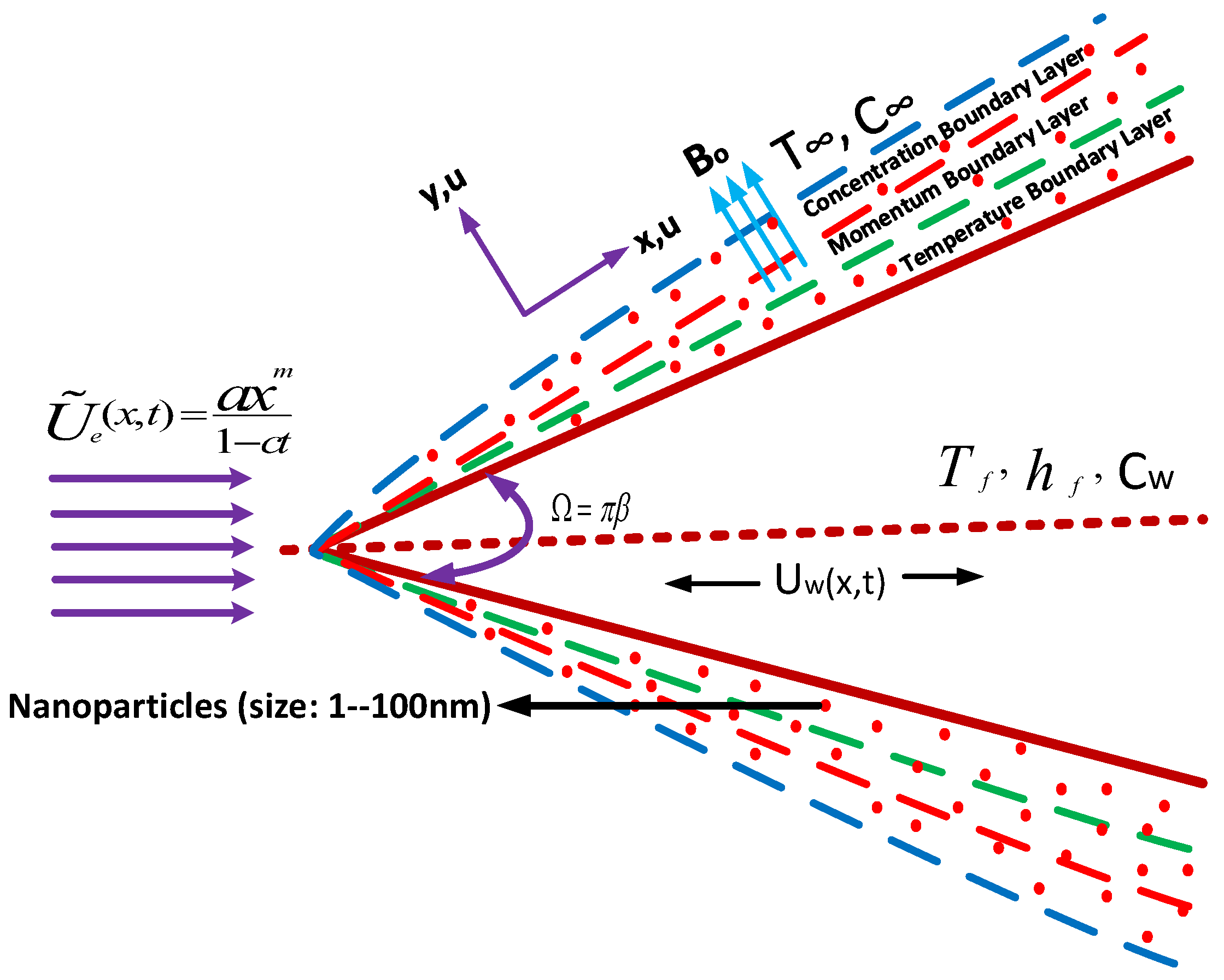
2.2. Statement of the Problem
3. Finite Element Solutions
3.1. Variational-Formulations
3.2. Formulation of Finite-Element


4. Results And Discussion
5. Conclusions
- Increased injection parameter makes the flow faster, whereas the suction causes the speed of flow to slow.
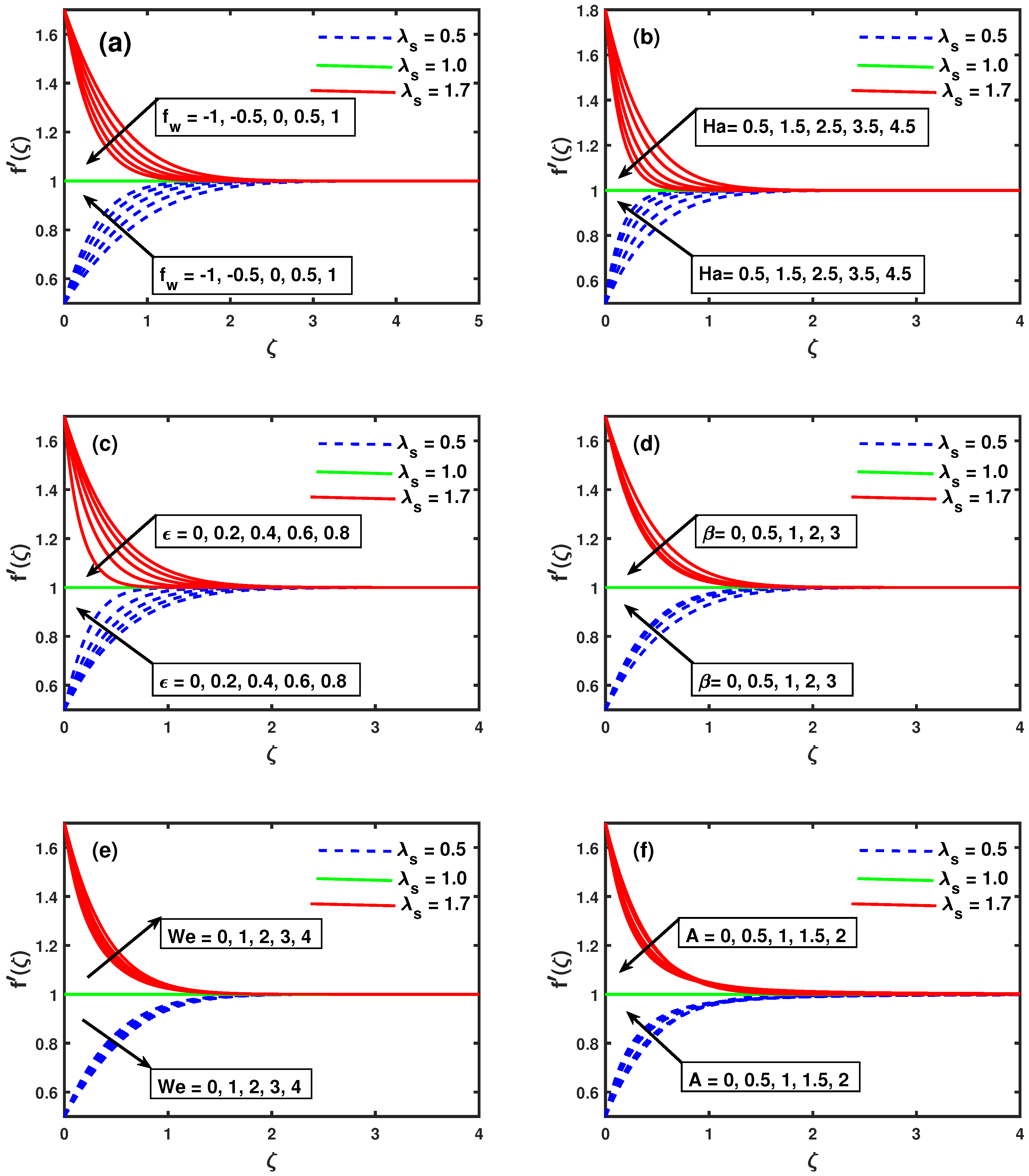
- The exceeding values of Hartman number , suction/injection material law index , aligned magnetic field parameter and unsteadiness parameter recede the velocity when whereas enhance when . An opposite trend is observed for Weissenberg number .
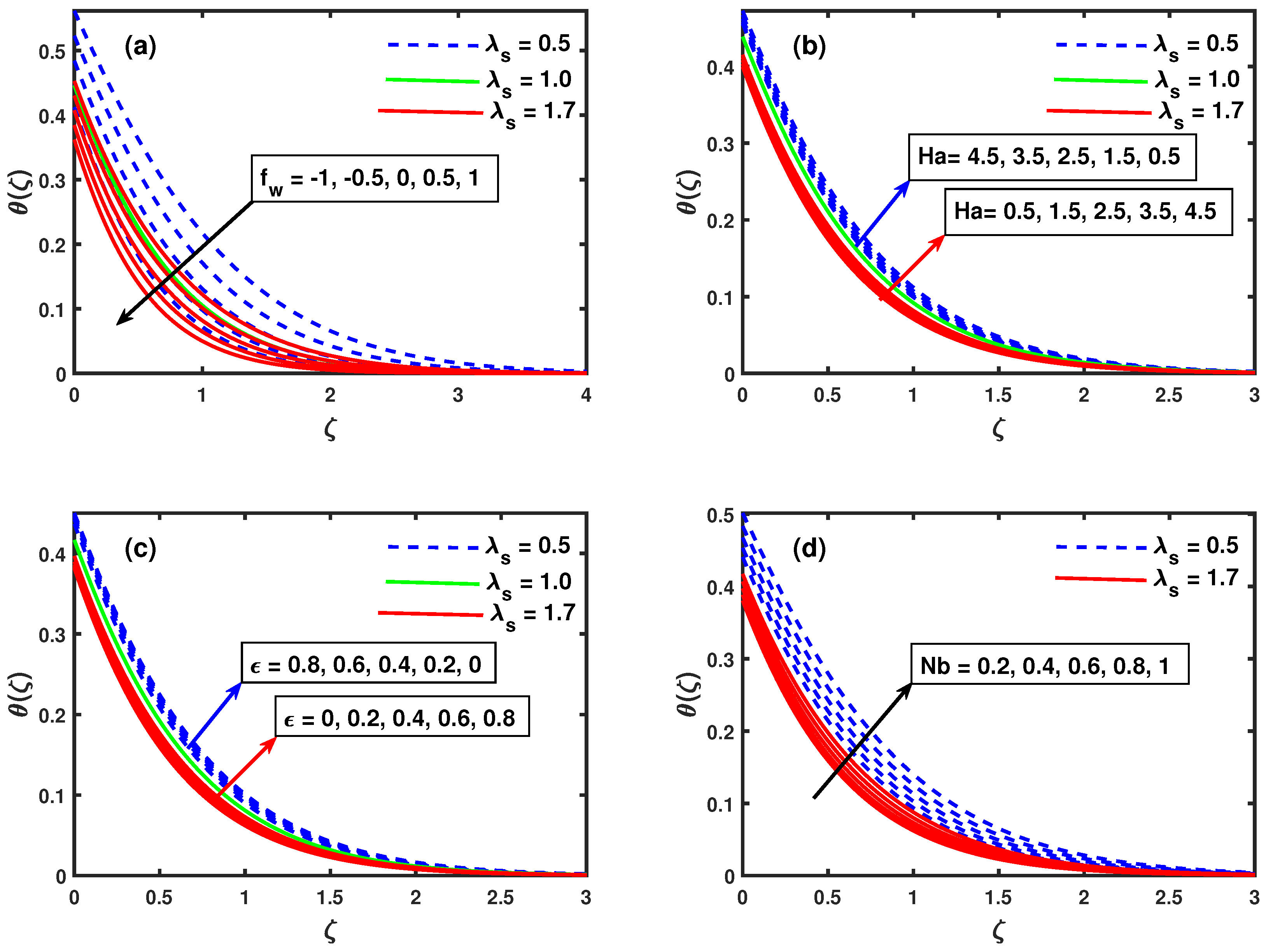
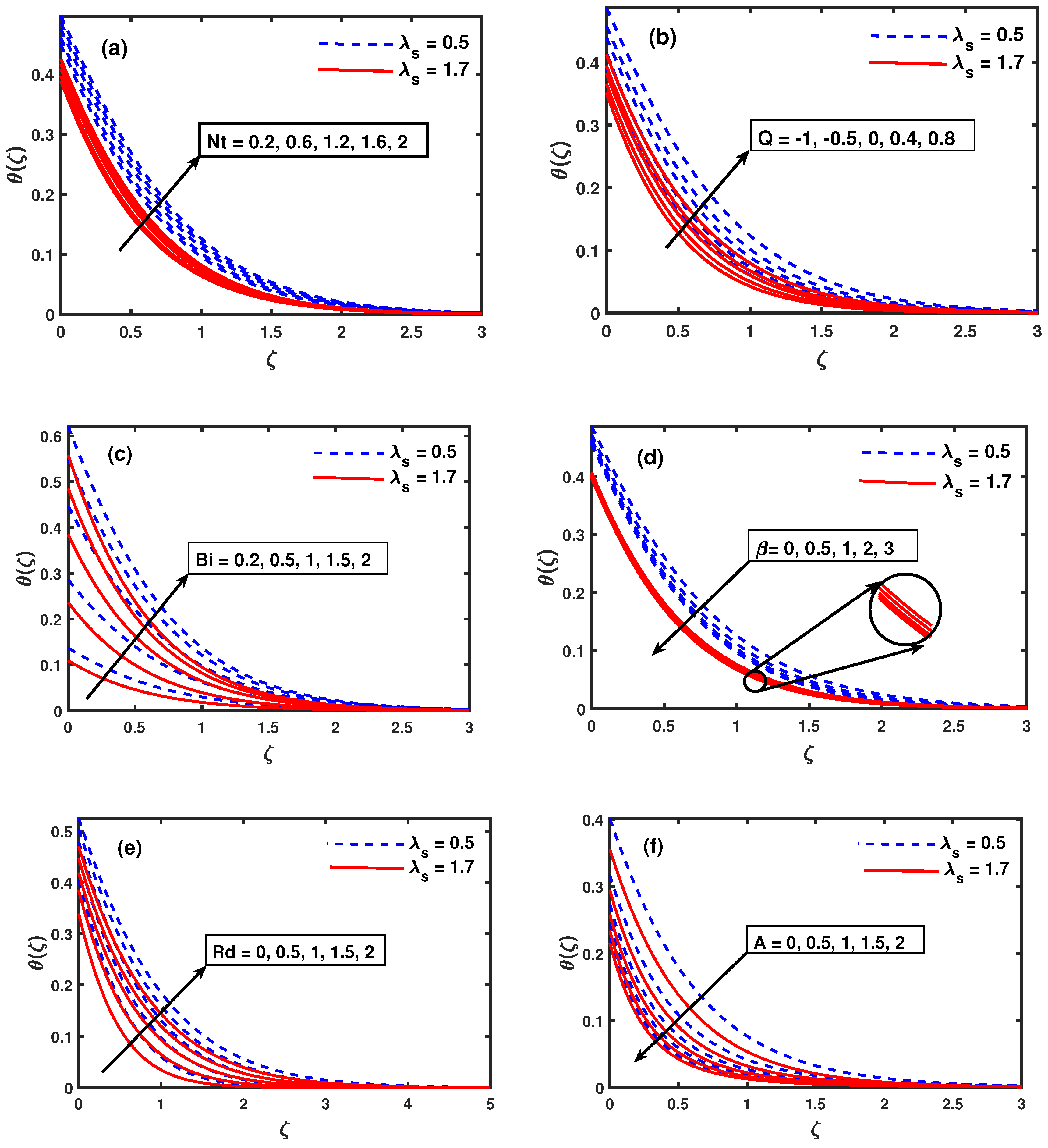
- The greater values of , , , Q and results in increased temperature distribution whereas the , , and unsteadiness causes it to decline in both cases ().
- The greater values of and results in increased temperature distribution when but a decline is observed for .
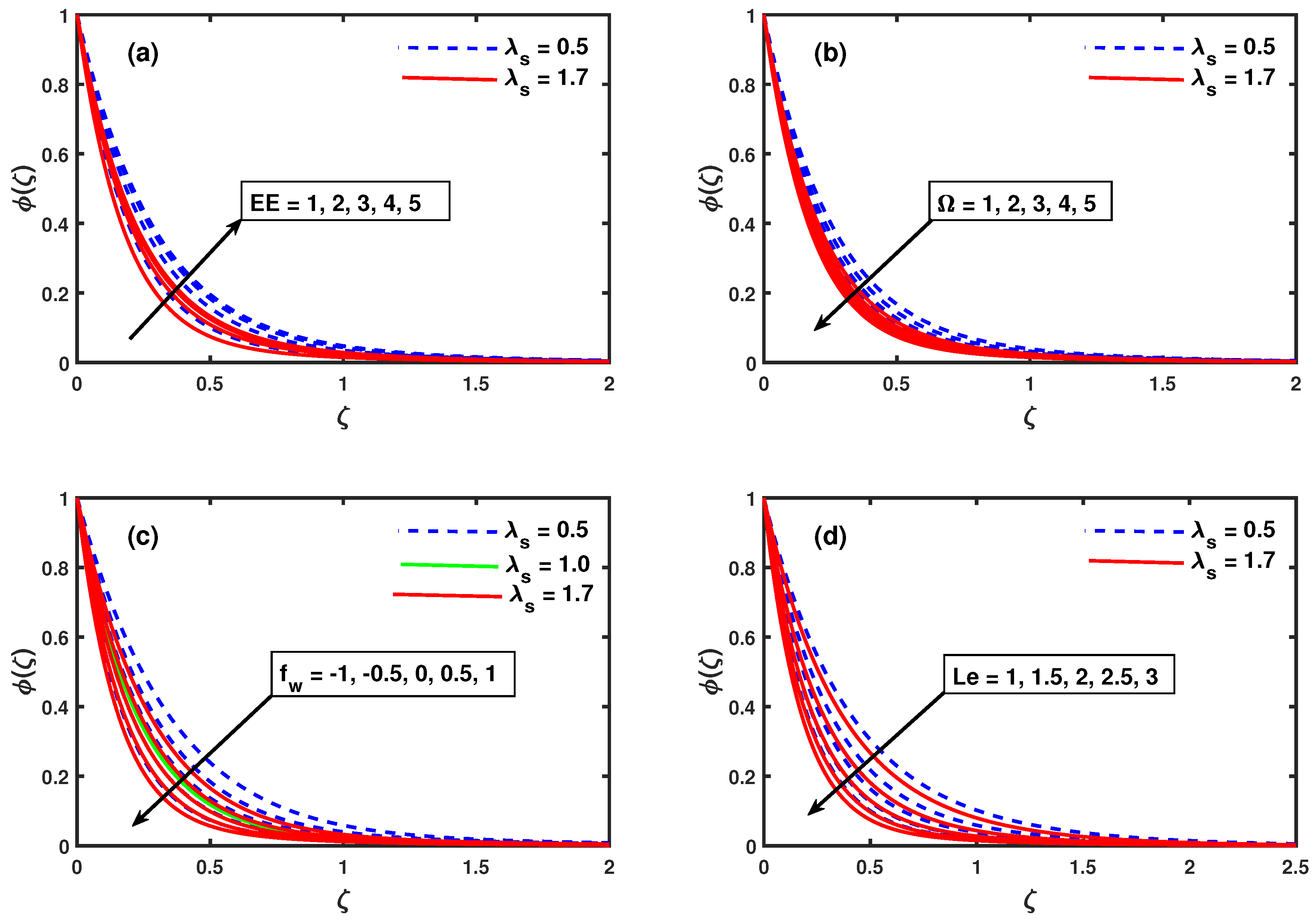
- The volume fraction of nanoparticles is upsurged with increment in but it diminishes against , and in both cases ().
- Skin friction grows larger with increment in values of when there is slow stretching , but the opposite pattern is observed for fast stretching .
- Nusselt number declines against progressive values of thermophoresis and Brownian motion parameters , .
Author Contributions
Funding
Acknowledgments
Conflicts of Interest
Nomenclature
| Non-dimensional temperature | |
| Temperature at surface | |
| Non-dimensional nanoparticles concentration | |
| Concentration at surface | |
| Temperature away from the surface | |
| Positive constants | |
| Concentration away from the surface | |
| E | Activation energy |
| Motile organisms away from the surface | |
| Velocity components | |
| Velocity of stretching/shrinking wedge | |
| Free stream velocity | |
| Thermal expansion coefficient | |
| Kinematic viscosity | |
| Density of fluid | |
| Prandtl number | |
| Thermophoretic diffusion coefficient | |
| Brownian diffusion coefficient | |
| m | Falkner-Skan power law |
| Uniform magnetic field | |
| Electrical conductivity | |
| Lewis number | |
| Wedge angle parameter | |
| Weissenberg number | |
| Base fluid heat capacity | |
| Heat generation/absorption | |
| E | Activation energy |
| Boltzmann constant | |
| n | Fitted rate constant |
| Stefan-Boltzmann number | |
| Mean assimilation coefficient | |
| Stream function | |
| Power law index | |
| Williamson parameter | |
| Brownian motion | |
| Thermophoresis | |
| chemical reaction rate | |
| Biot number | |
| Hartmann number | |
| Local Renolds number |
References
- Choi, S.U.; Eastman, J.A. Enhancing Thermal Conductivity of Fluids with Nanoparticles; Argonne National Lab.: Lemont, IL, USA, 1995. [Google Scholar]
- Buongiorno, J. Convective transport in nanofluids. J. Heat Transf. 2006, 128, 240–250. [Google Scholar] [CrossRef]
- Ibrahim, W.; Gamachu, D. Nonlinear convection flow of Williamson nanofluid past a radially stretching surface. AIP Adv. 2019, 9, 085026. [Google Scholar] [CrossRef]
- Khan, S.A.; Nie, Y.; Ali, B. Multiple slip effects on MHD unsteady viscoelastic nano-fluid flow over a permeable stretching sheet with radiation using the finite element method. SN Appl. Sci. 2020, 2, 66. [Google Scholar] [CrossRef] [Green Version]
- Manh, T.D.; Nam, N.D.; Abdulrahman, G.K.; Moradi, R.; Babazadeh, H. Impact of MHD on hybrid nanomaterial free convective flow within a permeable region. J. Therm. Anal. Calorim. 2019, 140, 2865–2873. [Google Scholar] [CrossRef]
- Abbas, S.; Khan, W.; Sun, H.; Ali, M.; Irfan, M.; Shahzed, M.; Sultan, F. Mathematical modeling and analysis of Cross nanofluid flow subjected to entropy generation. Appl. Nanosci. 2019, 10, 3149–3160. [Google Scholar] [CrossRef]
- Zadeh, S.M.H.; Mehryan, S.; Sheremet, M.A.; Izadi, M.; Ghodrat, M. Numerical study of mixed bio-convection associated with a micropolar fluid. Therm. Sci. Eng. Prog. 2020, 18, 100539. [Google Scholar]
- Hiemenz, K. Die Grenzschicht an einem in den gleichformigen Flussigkeitsstrom eingetauchten geraden Kreiszylinder. Dinglers Polytech. J. 1911, 326, 321–324. [Google Scholar]
- Awaludin, I.; Weidman, P.; Ishak, A. Stability analysis of stagnation-point flow over a stretching/shrinking sheet. AIP Adv. 2016, 6, 045308. [Google Scholar] [CrossRef]
- Merkin, J.H.; Pop, I. Stagnation point flow past a stretching/shrinking sheet driven by Arrhenius kinetics. Appl. Math. Comput. 2018, 337, 583–590. [Google Scholar] [CrossRef]
- Bhatti, M.M.; Abbas, M.A.; Rashidi, M.M. A robust numerical method for solving stagnation point flow over a permeable shrinking sheet under the influence of MHD. Appl. Math. Comput. 2018, 316, 381–389. [Google Scholar] [CrossRef]
- Shah, Z.; Kumam, P.; Deebani, W. Radiative MHD Casson Nanofluid Flow with Activation energy and chemical reaction over past nonlinearly stretching surface through Entropy generation. Sci. Rep. 2020, 10, 4402. [Google Scholar] [CrossRef] [Green Version]
- Fatunmbi, E.; Adeniyan, A. MHD stagnation point-flow of micropolar fluids past a permeable stretching plate in porous media with thermal radiation, chemical reaction and viscous dissipation. J. Adv. Math. Comput. Sci. 2018, 1–19. [Google Scholar] [CrossRef]
- Leal, L.G. Advanced Transport Phenomena: Fluid Mechanics and Convective Transport Processes; Cambridge University Press: Cambridge, UK, 2007; Volume 7. [Google Scholar]
- Falkneb, V.; Skan, S.W. LXXXV. Solutions of the boundary-layer equations. Lond. Edinb. Dublin Philos. Mag. J. Sci. 1931, 12, 865–896. [Google Scholar] [CrossRef]
- Ali, B.; Hussain, S.; Nie, Y.; Rehman, A.U.; Khalid, M. Buoyancy Effetcs On FalknerSkan Flow of a Maxwell Nanofluid Fluid with Activation Energy past a wedge: Finite Element Approach. Chin. J. Phys. 2020, 68, 368–380. [Google Scholar] [CrossRef]
- Watanabe, T. Thermal boundary layers over a wedge with uniform suction or injection in forced flow. Acta Mech. 1990, 83, 119–126. [Google Scholar] [CrossRef]
- Ishak, A.; Nazar, R.; Pop, I. MHD boundary-layer flow past a moving wedge. Magnetohydrodynamics 2009, 45, 103–110. [Google Scholar]
- Ali, B.; Hussain, S.; Nie, Y.; Khan, S.A.; Naqvi, S.I.R. Finite element simulation of bioconvection Falkner–Skan flow of a Maxwell nanofluid fluid along with activation energy over a wedge. Phys. Scr. 2020, 95, 095214. [Google Scholar] [CrossRef]
- Mohamed, R.; Rida, S.; Arafa, A.; Mubarak, M. Heat and Mass Transfer in an Unsteady Magnetohydrodynamics Al2O3—Water Nanofluid Squeezed Between Two Parallel Radiating Plates Embedded in Porous Media With Chemical Reaction. J. Heat Transf. 2020, 142, 012401. [Google Scholar] [CrossRef]
- Ali, B.; Rasool, G.; Hussain, S.; Baleanu, D.; Bano, S. Finite Element Study of Magnetohydrodynamics (MHD) and Activation Energy in Darcy–Forchheimer Rotating Flow of Casson Carreau Nanofluid. Processes 2020, 8, 1185. [Google Scholar] [CrossRef]
- Muhammad, T.; Waqas, H.; Khan, S.A.; Ellahi, R.; Sait, S.M. Significance of nonlinear thermal radiation in 3D Eyring–Powell nanofluid flow with Arrhenius activation energy. J. Therm. Anal. Calorim. 2020. [Google Scholar] [CrossRef]
- Kalaivanan, R.; Ganesh, N.V.; Al-Mdallal, Q.M. An investigation on Arrhenius activation energy of second grade nanofluid flow with active and passive control of nanomaterials. Case Stud. Therm. Eng. 2020, 22, 100774. [Google Scholar] [CrossRef]
- Shahzad, M.; Ali, M.; Sultan, F.; Khan, W.A.; Hussain, Z. Computational investigation of magneto-cross fluid flow with multiple slip along wedge and chemically reactive species. Results Phys. 2020, 16, 102972. [Google Scholar] [CrossRef]
- Hayat, T.; Waqas, M.; Alsaedi, A.; Bashir, G.; Alzahrani, F. Magnetohydrodynamic (MHD) stretched flow of tangent hyperbolic nanoliquid with variable thickness. J. Mol. Liq. 2017, 229, 178–184. [Google Scholar] [CrossRef]
- Mahdy, A.; Hoshoudy, G. EMHD time-dependant tangent hyperbolic nanofluid flow by a convective heated Riga plate with chemical reaction. Proc. Inst. Mech. Eng. Part E J. Process. Mech. Eng. 2019, 233, 776–786. [Google Scholar] [CrossRef]
- Zaib, A.; Haq, R.U.; Sheikholeslami, M.; Chamkha, A.J.; Rashidi, M.M. Impact of non-darcy medium on mixed convective flow towards a plate containing micropolar water-based tio 2 nanomaterial with entropy generation. J. Porous Media 2020, 23, 11–26. [Google Scholar] [CrossRef]
- Faraz, F.; Imran, S.M.; Ali, B.; Haider, S. Thermo-diffusion and multi-slip effect on an axisymmetric Casson flow over a unsteady radially stretching sheet in the presence of chemical reaction. Processes 2019, 7, 851. [Google Scholar] [CrossRef] [Green Version]
- Abbas, M.A.; Bhatti, M.M.; Sheikholeslami, M. Peristaltic propulsion of Jeffrey nanofluid with thermal radiation and chemical reaction effects. Inventions 2019, 4, 68. [Google Scholar] [CrossRef] [Green Version]
- Ali, L.; Xiaomin, L.; Ali, B.; Majeed, S.; Abdal, S. The Impact of Nanoparticles Due to Applied Magnetic Dipole in Micropolar Fluid Flow Using the Finite Element Method. Symmetry 2020, 12, 520. [Google Scholar] [CrossRef] [Green Version]
- Ramzan, M.; Gul, H.; Sheikholeslami, M. Effect of second order slip condition on the flow of tangent hyperbolic fluid—A novel perception of Cattaneo–Christov heat flux. Phys. Scr. 2019, 94, 115707. [Google Scholar] [CrossRef]
- Ali, L.; Xiaomin, L.; Ali, B.; Majeed, S.; Abdal, S.; Ali, S.K. Analysis of Magnetic Properties of Nano-Particles Due to a Magnetic Dipole in Micropolar Fluid Flow over a Stretching Sheet. Coatings 2020, 10, 170. [Google Scholar] [CrossRef] [Green Version]
- Ali, B.; Hussain, S.; Nie, Y.; Hussein, A.K.; Habib, D. Finite element investigation of Dufour and Soret impacts on MHD rotating flow of Oldroyd-B nanofluid over a stretching sheet with double diffusion Cattaneo Christov heat flux model. Powder Technol. 2021, 377, 439–452. [Google Scholar] [CrossRef]
- Ali, L.; Liu, X.; Ali, B.; Mujeed, S.; Abdal, S. Finite Element Analysis of Thermo-Diffusion and Multi-Slip Effects on MHD Unsteady Flow of Casson Nano-Fluid over a Shrinking/Stretching Sheet with Radiation and Heat Source. Appl. Sci. 2019, 9, 5217. [Google Scholar] [CrossRef] [Green Version]
- Ali, B.; Nie, Y.; Hussain, S.; Manan, A.; Sadiq, M.T. Unsteady magneto-hydrodynamic transport of rotating Maxwell nanofluid flow on a stretching sheet with Cattaneo–Christov double diffusion and activation energy. Therm. Sci. Eng. Prog. 2020, 20, 100720. [Google Scholar] [CrossRef]
- Ali, B.; Naqvi, R.A.; Hussain, D.; Aldossary, O.M.; Hussain, S. Magnetic Rotating Flow of a Hybrid Nano-Materials Ag-MoS2 and Go-MoS2 in C2H6O2-H2O Hybrid Base Fluid over an Extending Surface Involving Activation Energy: FE Simulation. Mathematics 2020, 8, 1730. [Google Scholar] [CrossRef]
- Shahzad, A.; Ali, R.; Hussain, M.; Kamran, M. Unsteady axisymmetric flow and heat transfer over time-dependent radially stretching sheet. Alex. Eng. J. 2017, 56, 35–41. [Google Scholar] [CrossRef] [Green Version]
- White, F.M. Viscous Fluid Flow; Magraw-Hill Inc.: New York, NY, USA, 1991. [Google Scholar]
- Ali, B.; Naqvi, R.A.; Nie, Y.; Khan, S.A.; Sadiq, M.T.; Rehman, A.U.; Abdal, S. Variable Viscosity Effects on Unsteady MHD an Axisymmetric Nanofluid Flow over a Stretching Surface with Thermo-Diffusion: FEM Approach. Symmetry 2020, 12, 234. [Google Scholar] [CrossRef] [Green Version]
- Ali, B.; Yu, X.; Sadiq, M.T.; Rehman, A.U.; Ali, L. A Finite Element Simulation of the Active and Passive Controls of the MHD Effect on an Axisymmetric Nanofluid Flow with Thermo-Diffusion over a Radially Stretched Sheet. Processes 2020, 8, 207. [Google Scholar] [CrossRef] [Green Version]
- Akbar, N.S.; Nadeem, S.; Haq, R.U.; Khan, Z. Numerical solutions of Magnetohydrodynamic boundary layer flow of tangent hyperbolic fluid towards a stretching sheet. Indian J. Phys. 2013, 87, 1121–1124. [Google Scholar] [CrossRef]
- Ilias, M.R.; Rawi, N.A.; Zaki, N.H.M.; Shafie, S. Aligned MHD Magnetic Nanofluid Flow Past a Static Wedge. Int. J. Eng. Technol. 2018, 7, 28–31. [Google Scholar] [CrossRef] [Green Version]
- Abdal, S.; Ali, B.; Younas, S.; Ali, L.; Mariam, A. Thermo-Diffusion and Multislip Effects on MHD Mixed Convection Unsteady Flow of Micropolar Nanofluid over a Shrinking/Stretching Sheet with Radiation in the Presence of Heat Source. Symmetry 2020, 12, 49. [Google Scholar] [CrossRef] [Green Version]
- Raju, C.; Hoque, M.M.; Sivasankar, T. Radiative flow of Casson fluid over a moving wedge filled with gyrotactic microorganisms. Adv. Powder Technol. 2017, 28, 575–583. [Google Scholar] [CrossRef]
- Ullah, I.; Shafie, S.; Khan, I. MHD heat transfer flow of Casson fluid past a stretching wedge subject to suction and injection. Malays. J. Fundam. Appl. Sci. 2017, 13, 637–641. [Google Scholar] [CrossRef] [Green Version]
- Reddy, G.J.; Raju, R.S.; Rao, J.A. Influence of viscous dissipation on unsteady MHD natural convective flow of Casson fluid over an oscillating vertical plate via FEM. Ain Shams Eng. J. 2018, 9, 1907–1915. [Google Scholar] [CrossRef]
- Jyothi, K.; Reddy, P.S.; Reddy, M.S. Carreau nanofluid heat and mass transfer flow through wedge with slip conditions and nonlinear thermal radiation. J. Braz. Soc. Mech. Sci. Eng. 2019, 41, 415. [Google Scholar] [CrossRef]
- Reddy, J.N. Solutions Manual for an Introduction to the Finite Element Method; McGraw-Hill: New York, NY, USA, 1993; p. 41. [Google Scholar]
- Ibrahim, W.; Gadisa, G. Finite element solution of nonlinear convective flow of Oldroyd-B fluid with Cattaneo-Christov heat flux model over nonlinear stretching sheet with heat generation or absorption. Propuls. Power Res. 2020, 55, 304–315. [Google Scholar] [CrossRef]
- Ali, B.; Hussain, S.; Abdal, S.; Mehdi, M.M. Impact of Stefan blowing on thermal radiation and Cattaneo–Christov characteristics for nanofluid flow containing microorganisms with ablation/accretion of leading edge: FEM approach. Eur. Phys. J. Plus 2020, 135, 1–18. [Google Scholar] [CrossRef]
- Ali, B.; Nie, Y.; Khan, S.A.; Sadiq, M.T.; Tariq, M. Finite Element Simulation of Multiple Slip Effects on MHD Unsteady Maxwell Nanofluid Flow over a Permeable Stretching Sheet with Radiation and Thermo-Diffusion in the Presence of Chemical Reaction. Processes 2019, 7, 628. [Google Scholar] [CrossRef] [Green Version]
- Khan, S.A.; Nie, Y.; Ali, B. Multiple Slip Effects on Magnetohydrodynamic Axisymmetric Buoyant Nanofluid Flow above a Stretching Sheet with Radiation and Chemical Reaction. Symmetry 2019, 11, 1171. [Google Scholar] [CrossRef] [Green Version]
- Uddin, M.; Rana, P.; Bég, O.A.; Ismail, A.M. Finite element simulation of magnetohydrodynamic convective nanofluid slip flow in porous media with nonlinear radiation. Alex. Eng. J. 2016, 55, 1305–1319. [Google Scholar] [CrossRef]
- Ibrahim, W.; Gadisa, G. Finite Element Method Solution of Boundary Layer Flow of Powell-Eyring Nanofluid over a Nonlinear Stretching Surface. J. Appl. Math. 2019, 2019, 3472518. [Google Scholar] [CrossRef]
- Ariel, P. Hiemenz flow in hydromagnetics. Acta Mech. 1994, 103, 31–43. [Google Scholar] [CrossRef]
- Ishak, A.; Nazar, R.; Pop, I. Falkner-Skan equation for flow past a moving wedge with suction or injection. J. Appl. Math. Comput. 2007, 25, 67–83. [Google Scholar] [CrossRef]
- Ahmad, R.; Khan, W.A. Effect of viscous dissipation and internal heat generation/absorption on heat transfer flow over a moving wedge with convective boundary condition. Heat Transf. Res. 2013, 42, 589–602. [Google Scholar] [CrossRef]
- Yih, K. MHD forced convection flow adjacent to a non-isothermal wedge. Int. Commun. Heat Mass Transf. 1999, 26, 819–827. [Google Scholar] [CrossRef]
- Ullah, I.; Shafie, S.; Khan, I. Heat generation and absorption in MHD flow of Casson fluid past a stretching wedge with viscous dissipation and newtonian heating. J. Teknol. 2018, 80, 1–9. [Google Scholar] [CrossRef] [Green Version]
- Postelnicu, A.; Pop, I. Falkner–Skan boundary layer flow of a power-law fluid past a stretching wedge. Appl. Math. Comput. 2011, 217, 4359–4368. [Google Scholar] [CrossRef]


| Number of Elements | ||||
|---|---|---|---|---|
| 60 | 1.068133 | 0.914246 | 0.148457 | 0.054075 |
| 100 | 1.067776 | 0.914217 | 0.148492 | 0.054118 |
| 180 | 1.067636 | 0.914206 | 0.148507 | 0.054136 |
| 360 | 1.067585 | 0.914202 | 0.148512 | 0.054142 |
| 500 | 1.067582 | 0.914202 | 0.148513 | 0.054143 |
| 700 | 1.067578 | 0.914201 | 0.148513 | 0.054144 |
| 1000 | 1.067575 | 0.914201 | 0.148513 | 0.054144 |
| Ariel [55] | Current Results | % Error | |||
|---|---|---|---|---|---|
| Perturbation Solution | Approximate Solution | (a) Exact Solution | (b) | ||
| 0.0 | 1.232588 | 1.224745 | 1.232588 | 1.232589 | 0.000081 |
| 0.4 | 1.295290 | 1.288410 | 1.295368 | 1.295369 | 0.000077 |
| 0.8 | 1.463725 | 1.462874 | 1.467976 | 1.467977 | 0.000068 |
| 1.0 | 1.570687 | 1.581139 | 1.585331 | 1.585332 | 0.000063 |
| 1.4 | 1.774774 | 1.840810 | 1.862848 | 1.862849 | 0.000161 |
| 1.6 | 1.842391 | 2.005172 | 2.017154 | 2.017155 | 0.000050 |
| 3.0 | - | 3.240355 | 3.240950 | 3.240952 | 0.000062 |
| 5.0 | - | 5.147815 | 5.147965 | 5.147968 | 0.000058 |
| 10.0 | - | 10.074740 | 10.074741 | 10.074748 | 0.000069 |
| Ishak [56] | Ahmadand Khan [57] | Yin [58] | Imran Ullaha [59] | Postelnicu and Pop [60] | FEM Current Results | |
|---|---|---|---|---|---|---|
| −1.0 | 0.7566 | 0.75655 | 0.75658 | 0.7566 | 0.75657 | 0.756576 |
| −0.5 | 0.9692 | 0.96922 | 0.96923 | 0.9692 | 0.96923 | 0.969232 |
| 0.0 | 1.2326 | 1.23258 | 1.23259 | 1.2326 | 1.23259 | 1.232591 |
| 0.5 | 1.5418 | 1.54175 | 1.54175 | 1.5418 | 1.54175 | 1.541756 |
| 1.0 | 1.8893 | 1.88931 | 1.88931 | 1.8893 | 1.88931 | 1.889321 |
| Pr | White [38] | FEM (Current Results) | ||
|---|---|---|---|---|
| 0.1 | 0.1980 | 0.2090 | 0.198129 | 0.209153 |
| 0.3 | 0.3037 | 0.3278 | 0.303719 | 0.327831 |
| 0.6 | 0.3916 | 0.4289 | 0.391677 | 0.428928 |
| 0.7 | 0.4178 | 0.4592 | 0.418094 | 0.459555 |
| 1.0 | 0.4696 | 0.5195 | 0.469604 | 0.519524 |
| 2.0 | 0.5972 | 0.6690 | 0.597241 | 0.669056 |
| 6.0 | 0.8672 | 0.9872 | 0.867297 | 0.987299 |
| 10.0 | 1.0297 | 1.1791 | 1.029779 | 1.179182 |
Publisher’s Note: MDPI stays neutral with regard to jurisdictional claims in published maps and institutional affiliations. |
© 2020 by the authors. Licensee MDPI, Basel, Switzerland. This article is an open access article distributed under the terms and conditions of the Creative Commons Attribution (CC BY) license (http://creativecommons.org/licenses/by/4.0/).
Share and Cite
Ali, B.; Naqvi, R.A.; Mariam, A.; Ali, L.; Aldossary, O.M. Finite Element Study for Magnetohydrodynamic (MHD) Tangent Hyperbolic Nanofluid Flow over a Faster/Slower Stretching Wedge with Activation Energy. Mathematics 2021, 9, 25. https://0-doi-org.brum.beds.ac.uk/10.3390/math9010025
Ali B, Naqvi RA, Mariam A, Ali L, Aldossary OM. Finite Element Study for Magnetohydrodynamic (MHD) Tangent Hyperbolic Nanofluid Flow over a Faster/Slower Stretching Wedge with Activation Energy. Mathematics. 2021; 9(1):25. https://0-doi-org.brum.beds.ac.uk/10.3390/math9010025
Chicago/Turabian StyleAli, Bagh, Rizwan Ali Naqvi, Amna Mariam, Liaqat Ali, and Omar M. Aldossary. 2021. "Finite Element Study for Magnetohydrodynamic (MHD) Tangent Hyperbolic Nanofluid Flow over a Faster/Slower Stretching Wedge with Activation Energy" Mathematics 9, no. 1: 25. https://0-doi-org.brum.beds.ac.uk/10.3390/math9010025