Vector Geometric Algebra in Power Systems: An Updated Formulation of Apparent Power under Non-Sinusoidal Conditions

Abstract

Traditional electrical power theories and one of their most important concepts—apparent power—are still a source of debate, because they present several flaws that misinterpret the power-transfer and energy-balance phenomena under distorted grid conditions. In recent years, advanced mathematical tools such as geometric algebra (GA) have been introduced to address these issues. However, the application of GA to electrical circuits requires more consensus, improvements and refinement. In this paper, electrical power theories for single-phase systems based on GA were revisited. Several drawbacks and inconsistencies of previous works were identified, and some amendments were introduced. An alternative expression is presented for the electric power in the geometric domain. Its norm is compatible with the traditional apparent power defined as the product of the RMS voltage and current. The use of this expression simplifies calculations such as those required for current decomposition. This proposal is valid even for distorted currents and voltages. Concepts are presented in a simple way so that a strong background on GA is not required. The paper included some examples and experimental results in which measurements from a utility supply were analysed.

1. Introduction

The full understanding of power flows in electrical and electronic systems has been a topic of interest during the last century. It is of paramount relevance because of the increasing energy losses in transmission systems, as well as the the poor power quality on electrical devices. In particular, the reduction of power losses involves the reduction of ${\mathrm{CO}}_2$ emissions. This aim requires the installation of smart metering systems in the grid to collect a large amount of electrical power data [1]. To accomplish this task, relevant efforts have been carried out in the frequency domain for systems operating in steady state [2] and in the time domain by using both instantaneous and averaged approaches [3,4,5]. The outcomes from these studies were sometimes inconsistent and even contradictory. For example, the well-known instantaneous power theory can yield incoherent results under specific conditions [6]. Similar controversial results have been found for well-established regulations such as the standard IEEE 1459 [7]. Traditional techniques that are commonly applied for analysing power flows are based on linear algebra tools such as complex numbers, matrices, tensors, etc., and they have been proven to be useful from the application point of view [8]. However, none of them provide a clear overview of power flows under disported and unbalanced grid conditions, and this point is still an open discussion [9]. Geometric algebra (GA) is a mathematical tool developed by W. K. Clifford and H. Grassmann at the end of the 19th Century. It has been rediscovered and refined in the last few decades by Hestenes [10] and others [11]. This tool has brought new possibilities to important fields such as physics [10], computer graphics [12] and rendering problems [13], producing compact and generalised formulations [14]. Furthermore, it can be easily used to manipulate integral and differential equations in multi-component systems [15,16]. Even though GA is not widely known by the scientific community, it has a great potential and has attracted a lot of interest in recent publications [17]. GA has already been introduced to reformulate the apparent power as the geometric product between voltage and current, which is commonly written as $\mathit{M}$ [18,19,20,21]. Compared to the traditional definition of apparent power $S=VI$, the use of $\mathit{M}$ has several advantages. A relevant one is that $\mathit{M}$ is conservative in spite of S, and this is of interest for its application in distorted environments [22]. The use of a different letter $\mathit{M}$ instead of the traditional one S is therefore justified. It also has important implications for the definition of reactive power and its compensation, and this is a topic of interest for the power community [23].

Contributions

The main contributions and novelties of this paper are based on the following points:

• GA power theories proposed by different authors were briefly reviewed in order to analyse some of the inconsistencies raised so far, while additional ones not yet found in the literature were also discussed [7,18,24]. Menti’s pioneering expression for geometric electric power was recovered because it has several advantages and benefits over other proposals for power computations. For example, one of the most relevant is that its norm equals the product between the norms of geometric voltage and current, thus retaining the traditional approach in the apparent power definition. It should be emphasized that this approach is different from those already published and based on k-blades or complex-vectors;
• A new mapping between the Fourier basis for periodic time functions and the Euclidean basis was introduced, accounting for harmonics, inter- and sub-harmonics and DC components. Because no additional restrictions were imposed on the waveforms, the developed methodology is valid even in the case of distorted currents and voltages. Furthermore, the relevant features of GA for power and circuit analysis and power calculations were maintained: electrical circuits can be easily solved, and the principle of energy conservation was still satisfied;
• Another relevant contribution was the formulation by means of vectors in GA for some of the most important laws in basic circuit theory, i.e., Kirchoff’s laws or Ohm’s law, to mention a few. This is a crucial issue when solving steady-state AC circuits in GA without the use of complex phasors. The concept of geometrical impedance as a bivector was also introduced;
• Another very relevant aspect is the current decomposition proposal based on the use of the inverse of the voltage vector, which has important implications in the use of active filters and current compensation. It was shown that the use of this approach allowed a comprehensive current decomposition for optimal passive/active filtering based on the concept of the vector inverse, not discussed previously in the literature.

Numerical and experimental results were included in order to validate the main contributions of this work. A brief introduction to GA and its terminology was included in order to make the paper self-contained.

2. Geometric Algebra for Power Flow Analysis

The geometric product was introduced by Clifford at the end of the 19th Century, and it includes the exterior (Grassmann) and interior (dot) products of vectors. Suppose a Euclidean two-dimensional vector space ${\mathbb{R}}^2$ spanned by the basis $\{{\mathit{\sigma }}_1,{\mathit{\sigma }}_2\}$ and elements such as $\mathit{a}={\alpha }_1{\mathit{\sigma }}_{\mathbf{1}}+{\alpha }_2{\mathit{\sigma }}_{\mathbf{2}}$ and $\mathit{b}={\beta }_1{\mathit{\sigma }}_{\mathbf{1}}+{\beta }_2{\mathit{\sigma }}_{\mathbf{2}}$ with ${\alpha }_i,{\beta }_i\in \mathbb{R}$. Their interior product can be calculated as follows:

$$\mathit{a}·\mathit{b}=\parallel \mathit{a}\parallel \parallel \mathit{b}\parallel cos\phi =\sum {\alpha }_i{\beta }_i$$

(1)

while the exterior product is:

$$\mathit{a}\wedge \mathit{b}=\parallel \mathit{a}\parallel \parallel \mathit{b}\parallel sin\phi {\mathit{\sigma }}_{\mathbf{1}}{\mathit{\sigma }}_{\mathbf{2}}$$

(2)

The operation in Equation (2) does not exist in traditional linear algebra, and its result is not a scalar, nor a vector, but a new entity that is commonly known as a bivector [10]. Bivectors play a key role in calculations related to non-active power, as is shown later. The exterior product is anticommutative, i.e., $\mathit{a}\wedge \mathit{b}=-\mathit{b}\wedge \mathit{a}$. The fundamental operation in GA is the geometric product:

$$\begin{array}{cc}\hfill \mathit{M}=\mathit{a}\mathit{b}& =({\alpha }_1{\mathit{\sigma }}_{\mathbf{1}}+{\alpha }_2{\mathit{\sigma }}_{\mathbf{2}})({\beta }_1{\mathit{\sigma }}_{\mathbf{1}}+{\beta }_2{\mathit{\sigma }}_{\mathbf{2}})=\underset{{\langle \mathit{M}\rangle }_0}{\underbrace{({\alpha }_1{\beta }_1+{\alpha }_2{\beta }_2)}}+\underset{{\langle \mathit{M}\rangle }_2}{\underbrace{({\alpha }_1{\beta }_2-{\alpha }_2{\beta }_1)}}{\mathit{\sigma }}_{\mathbf{1}}{\mathit{\sigma }}_{\mathbf{2}}\hfill \end{array}$$

(3)

where $\mathit{M}$ consists of two elements. As these elements are of a different nature, $\mathit{M}$ is commonly referred to as a multivector. The operation ${\langle \mathit{X}\rangle }_k$ refers to the extraction of the k-grade component of a multivector $\mathit{X}$. In Equation (3), the term ${\langle \mathit{M}\rangle }_0$ is a scalar, while the term ${\langle \mathit{M}\rangle }_2$ is a bivector. Multivectors are classified according to their degree: scalars have degree zero, vectors one, bivectors two, etc. The norm of a multivector is:

$$\parallel \mathit{M}\parallel =\sqrt{{\langle {\mathit{M}}^{†}\mathit{M}\rangle }_0}$$

(4)

where ${\mathit{M}}^{†}$ is the reverse of $\mathit{M}$ (see [10] for details). Note that in the rest of this work, vectors are represented by bold lower case letters while bivectors and multivectors are represented by bold upper case letters. Considering a single-phase system operating under perfect periodic sinusoidal conditions, it is possible to select an orthonormal basis in the space vector of Fourier functions:

$$\mathit{\phi }=\{1,\sqrt{2}cos\omega t,\sqrt{2}sin\omega t\}$$

(5)

This basis also belongs to the $L^2$ Hilbert space [25] of integrable and finite energy functions, equipped with a norm:

$$\parallel x\left(t\right)\parallel =\sqrt{\frac{1}{T}{\int }_0^T{x}^2\left(t\right)dt}$$

(6)

Note that $x\left(t\right)$ can be expressed as a linear combination of the orthonormal elements ${\mathit{\phi }}_j$ with $j=1,2,3$ as in $x\left(t\right)={\sum }_{j=1}^3{x}_j{\phi }_j\left(t\right)$, which, in general, can be represented in a Euclidean vector space as a vector $\mathit{x}={\sum }_{j=1}^3{x}_j{\sigma }_{\mathbf{j}}$ as defined previously. The above can be readily extended to non-sinusoidal signals by updating the basis to $\mathit{\phi }={\{1,\sqrt{2}cosk\omega t,\sqrt{2}sink\omega t\}}_{k=1}^n$ where n is the number of harmonics under consideration. For simplicity, the DC term will not be considered at this moment (but it can be added without problems). Therefore, voltages and currents are transformed to the proposed Euclidean vector space as follows:

$$\begin{array}{cccc}\hfill u\left(t\right)& ⟶\hfill & \hfill \mathit{u}& ={\alpha }_1{\mathit{\sigma }}_{\mathbf{1}}+{\alpha }_2{\mathit{\sigma }}_{\mathbf{2}}\hfill \\ \hfill i\left(t\right)& ⟶\hfill & \hfill \mathit{i}& ={\beta }_1{\mathit{\sigma }}_{\mathbf{1}}+{\beta }_2{\mathit{\sigma }}_{\mathbf{2}}\hfill \end{array}$$

(7)

The geometric product defined in Equation (3) can be used to calculate the geometric power:

$$\mathit{M}=\mathit{u}\mathit{i}=\underset{P}{\underbrace{({\alpha }_1{\beta }_1+{\alpha }_2{\beta }_2)}}+\underset{\mathit{Q}}{\underbrace{({\alpha }_1{\beta }_2-{\alpha }_2{\beta }_1){\mathit{\sigma }}_{\mathbf{1}}{\mathit{\sigma }}_{\mathbf{2}}}}$$

(8)

This expression consists of two terms of a different nature that can be clearly identified: P is a scalar, and $\mathit{Q}$ is a bivector. Note that $\parallel \mathit{Q}\parallel$ is the traditional reactive power Q. For convenience, ${\mathit{\sigma }}_1{\mathit{\sigma }}_2$ is often written as ${\mathit{\sigma }}_{12}$. This result is extended to non-sinusoidal conditions in later sections. The geometric power fulfils:

$${\parallel \mathit{M}\parallel }^2={\langle \mathit{M}\rangle }_0^2+{\langle \mathit{M}\rangle }_2^2=P^2+Q^2={\parallel \mathit{u}\parallel }^2{\parallel \mathit{i}\parallel }^2$$

(9)

3. GA-Based Power Theories: Overview

In this section, the main power theories based on GA are briefly and critically discussed so that the main contributions of this paper can be better understood.

• Menti: This theory was developed by Anthoula Menti et al. in 2007 [18]. This was the first application of GA to electrical circuits. The apparent power multivector was defined by multiplying the voltage and current in the geometric domain:

  $$\mathit{S}=\mathit{u}\mathit{i}=\mathit{u}·\mathit{i}+\mathit{u}\wedge \mathit{i}={〈\mathit{S}〉}_0+{〈\mathit{S}〉}_2$$

  (10)
  The scalar part matches the active power P, while the bivector part represents power components with zero mean value. Unfortunately, the theory did not establish a general framework for the resolution of electrical circuits under distorted conditions. Furthermore, the proposal was not applied to decompose currents (for non-linear load compensation, for example), and it was not extended to multi-phase systems.
• Castilla–Bravo: This theory was developed by Castilla and Bravo in 2008 [19]. The authors introduced the concept of generalised complex geometric algebra. Vector-phasors were defined for both voltage and current:

  $$\begin{array}{c}\hfill {\tilde{\mathit{U}}}_p=U_p{e}^{j{\alpha }_p}{\mathit{\sigma }}_p={\overline{U}}_p{\mathit{\sigma }}_p,{\tilde{\mathit{I}}}_q=I_q{e}^{j{\beta }_q}{\mathit{\sigma }}_q={\overline{I}}_q{\mathit{\sigma }}_q\end{array}$$

  (11)
  Geometric power results from multiplying the harmonic voltage and conjugated harmonic current vector-phasors:

  $$\tilde{\mathit{S}}=\sum _{\begin{array}{c}p\in N\cup L\\ q\in N\cup M\end{array}}{\tilde{\mathit{U}}}_p{\tilde{\mathit{I}}}_q^{*}=\tilde{P}+j\tilde{Q}+\tilde{D}$$

  (12)
  This proposal is able to capture the multicomponent nature of apparent power through the so-called complex scalar $\tilde{P}+j\tilde{Q}$ and the complex bivector $\tilde{D}$. However, this formulation requires the use of complex numbers, which could have been avoided by using appropriate bivectors [14]. Furthermore, only definitions of powers were presented, and it was not extended to multi-phase systems.
• Lev-Ari: This theory was developed by Lev-Ari [20,26], and it was the first application of GA to multi-phase systems in the time domain. However, this work did not contain examples, nor fundamentals for load compensation. Furthermore, practical aspects required to solve electrical circuits were not explained.
• Castro-Núñez: This theory was developed by Castro-Núñez in the year 2010 [27] and then extended and refined in further works [7,28]. A relevant contribution of this work consisted of the resolution of electrical circuits by using GA (without requiring complex numbers). Furthermore, a multivector called geometric power that is conservative and fulfils the Tellegen theorem was defined [29]. As in the Menti and Castilla–Bravo proposals, the results were presented only for single-phase systems. Another contribution was the definition of a transformation based on k-blades, i.e., objects that can be expressed as the exterior product of k basis vectors. They form an orthonormal base. However, this basis presents some drawbacks. The main one is the definition of the geometric power [30]. In particular, active power calculations did not match with those obtained by using classical theories. Therefore, the authors needed to include an ad hoc corrective coefficient [7]. Finally, the definition of geometric power norm did not follow the traditional expression as a product or voltage and current norms (i.e., RMS in the complex domain) due to the proposed axiomatic transformation.
• Montoya: This framework was proposed by Montoya et al. [30], and it is an upgrade of the Menti and Castro-Núñez theories [7,18]. It establishes a general framework for power calculations in the frequency domain. Since it was the most recent work, it provided solutions to some problems detected so far in other proposals, and the formulation was more compact and efficient. However, this framework was based on the use of k-blades, and therefore, drawbacks related to the non-standardised definition of apparent power were inherited from previous theories.

The most relevant contributions of this work compared to existing proposals are presented in

Table 1. Comparison of the main contributions of GA power theories.

Feature	Menti [18]	Castilla and Bravo [19]	Lev-Ari [20]	Castro-Núñez [27]	Montoya [21]	This Work
Based on	vectors	complex-vectors	vectors	k-blades	k-blades	vectors
GA power definition	$\mathit{S}=\mathit{u}\mathit{i}$	$\tilde{S}=\sum {\tilde{U}}_p\widehat{g}{\tilde{I}}_q^{*}$	$\mathbb{S}=\mathbf{v}\mathbf{i}$	$M=VI$	$\mathit{M}={\mathit{VI}}^{†}$	$\mathit{M}=\mathit{u}\mathit{i}$
Power norm	$\parallel \mathit{S}\parallel =\parallel \mathit{u}\parallel \parallel \mathit{i}\parallel$	$|\tilde{S}{|}^2=|\tilde{U}{|}^2{|\tilde{I}|}^2$	$\parallel \mathbb{S}\parallel =\parallel \mathbf{v}\parallel \parallel \mathbf{i}\parallel$	$\parallel M\parallel \ne \parallel V\parallel \parallel I\parallel$	$\parallel \mathit{M}\parallel \ne \parallel \mathit{V}\parallel \parallel {\mathit{I}}^{†}\parallel$	$\parallel \mathit{M}\parallel =\parallel \mathit{u}\parallel \parallel \mathit{i}\parallel$
Circuit theory ready	No	No	No	Yes	Yes	Yes
Current decomposition	No	No	No	No	Not Always	Yes
Interharmonic handling	No	No	No	No	Yes	Yes
Impedance definition	No	No	No	Yes	Yes	Yes

.

4. GA Framework and Methodology

4.1. Circuit Analysis by Means of GA

In this theory, different approaches already available in the literature are unified and enhanced in order to analyse electrical circuits in the geometric domain. The proposed modifications are deemed to remain consistent with the physical basic principles observed in electrical circuits. An orthonormal basis $\mathit{\sigma }=\{{\mathit{\sigma }}_1,{\mathit{\sigma }}_2,\dots ,{\mathit{\sigma }}_n\}$ is used in order to represent the multi-component nature of periodic signals with finite energy. Consider a voltage signal $u\left(t\right)$:

$$\begin{array}{cc}\hfill u\left(t\right)& =U_0+\sqrt{2}{\sum }_{k=1}^n{U}_{k}cos(k\omega t+{\phi }_k)+\sqrt{2}{\sum }_{l\in L}{U}_{l}cos(l\omega t+{\phi }_l)\hfill \end{array}$$

(13)

where $U_0$ is the DC component, while $U_k$ and ${\phi }_k$ are the RMS and phase of the k-th harmonic, respectively. The set L represents sub- and inter-harmonics included in the signal [31]. As in traditional circuit analysis based on complex variables, a sinusoidal and steady-state signal can be considered as a part of a rotating vector $\mathit{n}\left(t\right)$ (in a similar fashion to $e^{j\omega t}$). It was demonstrated that this facilitated the analysis in the geometric domain. In addition, thanks to the linear properties of GA, it was possible to define a single multivector that included all the harmonic frequencies present in the signal (this was not possible by using the traditional complex analysis). This rotating vector $\mathit{n}\left(t\right)$ in a two-dimensional geometric space ${\mathcal{G}}_2$ can be obtained as follows [32]:

$$\begin{array}{cc}\hfill \mathit{n}\left(t\right)& =e^{\frac{1}{2}\omega t{\mathit{\sigma }}_{12}}\mathit{N}{e}^{-\frac{1}{2}\omega t{\mathit{\sigma }}_{12}}=\mathit{R}\mathit{N}{\mathit{R}}^{†}=e^{\omega t{\mathit{\sigma }}_{12}}\mathit{N}={\mathit{R}}^2\mathit{N}=\mathit{N}{\mathit{R}}^{†2}\hfill \end{array}$$

(14)

where $\mathit{R}=e^{\frac{1}{2}\omega t{\mathit{\sigma }}_{12}}$ is a geometric rotor (or simply a rotor) [33] and $\mathit{N}$ is a vector. In Equation (14), left-multiplying produces opposite effects compared to right-multiplying. Figure 1 shows a graphical representation of a vector $\mathit{N}$ left-multiplied by a rotor ${\mathit{R}}^{\prime }=e^{\phi {\mathit{\sigma }}_{12}}$ with positive angle $\phi$. This operation produces a rotated vector (in green) in clockwise direction. Similarly, the same vector $\mathit{N}$ right-multiplied by the same rotor ${\mathit{R}}^{\prime }$ produces a rotation of $\phi$ degrees in the counter-clockwise direction (vector in red).

In order to maintain the commonly accepted convention of signs in electrical engineering, vectors are always left-multiplied by rotors. Therefore, a positive sign in a phase angle refers to the clockwise direction. This implies that an inductor reactance will have positive phase angles, while a capacitor will have negative phase angles. However, the phase lead and lag now change its role in the geometric domain: lag implies rotation in the counter-clockwise direction and lead in the clockwise direction (see Figure 1).

It can be proven that the projection of a rotating vector voltage ${\mathit{u}}_1\left(t\right)$ over the basis ${\mathit{\sigma }}_1$ yields the original voltage waveform, i.e., $u_1\left(t\right)=\sqrt{2}({\alpha }_{1}cos\omega t+{\alpha }_{2}sin\omega t)$. This resembles the extraction of the real part of a complex rotating phasor, i.e., $\mathcal{R}e\left\{\sqrt{2}\overrightarrow{\mathit{V}}{e}^{j\omega t}\right\}$. By using the Euclidean orthonormal basis $\mathit{\sigma }=\{{\mathit{\sigma }}_1,{\mathit{\sigma }}_2\}$ isomorphic to the Fourier basis in Equation (5), then the original time signal $u_1\left(t\right)$ is transformed into the vector ${\mathit{u}}_1={\alpha }_1{\mathit{\sigma }}_1+{\alpha }_2{\mathit{\sigma }}_2$; therefore:

$$\begin{array}{cc}& {\mathit{u}}_1\left(t\right)=e^{\omega t{\mathit{\sigma }}_{12}}{\mathit{u}}_1=(cos\omega t+sin\omega t{\mathit{\sigma }}_{12})({\alpha }_1{\mathit{\sigma }}_1+{\alpha }_2{\mathit{\sigma }}_2)=\hfill \\ & =\left({\alpha }_{1}cos\omega t+{\alpha }_{2}sin\omega t\right){\mathit{\sigma }}_1+\left({\alpha }_{2}cos\omega t-{\alpha }_{1}sin\omega t\right){\mathit{\sigma }}_2\hfill \\ & =\frac{1}{\sqrt{2}}\left(u_1\left(t\right){\mathit{\sigma }}_1-\mathcal{H}\left[u_1\left(t\right)\right]{\mathit{\sigma }}_2\right)\hfill \end{array}$$

(15)

where $\mathcal{H}$ refers to the Hilbert transform of a signal [34]. Hence, $u_1\left(t\right)={proj}_{{\mathit{\sigma }}_1}\left[\sqrt{2}{\mathit{u}}_1\left(t\right)\right]=\sqrt{2}{\mathit{u}}_1\left(t\right)·{\mathit{\sigma }}_1$ can be recovered as the scalar product, i.e., the projection of a rotating vector ${\mathit{u}}_1\left(t\right)$ onto ${\mathit{\sigma }}_1$. It is worth pointing out that the rotating vector ${\mathit{u}}_1\left(t\right)$ is not the original time domain voltage waveform, $u_1\left(t\right)$. This is a different interpretation compared to that of other authors [7,22]. This discrepancy was analysed by using the simple RLC circuit depicted in Figure 2. Its solution is well known in both the time and complex domain (for the steady state), but it is presented here to highlight that the proposed framework can be applied to the most basic electrical circuits. The time-domain equation that governs the circuit dynamics is:

$$u_1\left(t\right)=Ri\left(t\right)+L\frac{di\left(t\right)}{dt}+\frac{1}{C}\int i\left(t\right)dt$$

(16)

If we perform the derivative and the integral [32] of the rotating vector defined in Equation (15), we obtain:

$$\begin{array}{cc}\hfill \frac{d{\mathit{u}}_1\left(t\right)}{dt}& =\omega {\mathit{\sigma }}_{12}{\mathit{u}}_1\left(t\right)\hfill \\ \hfill \int {\mathit{u}}_1\left(t\right)dt& =-\frac{{\mathit{\sigma }}_{12}}{\omega }{\mathit{u}}_1\left(t\right)\hfill \end{array}$$

(17)

Because the source is sinusoidal and assuming that the circuit is operating in the steady state, Equation (15) can be substituted in Equation (16),

$$\begin{array}{cc}\hfill {proj}_{{\mathit{\sigma }}_1}\left[\sqrt{2}{e}^{\omega t{\mathit{\sigma }}_{12}}{\mathit{u}}_1\right]& =\sqrt{2}{proj}_{{\mathit{\sigma }}_1}\left[R{e}^{\omega t{\mathit{\sigma }}_{12}}\mathit{i}+L\omega {\mathit{\sigma }}_{12}{e}^{\omega t{\mathit{\sigma }}_{12}}\mathit{i}-\frac{{\mathit{\sigma }}_{12}}{C\omega }{e}^{\omega t{\mathit{\sigma }}_{12}}\mathit{i}\right]\hfill \end{array}$$

(18)

so, applying the same rationale used in Equation (15), Equation (18) can be simplified, yielding:

$${\mathit{u}}_1=R\mathit{i}+L\omega {\mathit{\sigma }}_{12}\mathit{i}-\frac{{\mathit{\sigma }}_{12}}{C\omega }\mathit{i}$$

(19)

Rotors such as $e^{\omega t{\mathit{\sigma }}_{12}}$ are cancelled out because they commute with ${\mathit{\sigma }}_{12}$. Therefore, it is not necessary to set any specific time instant $t_0$ after performing the derivative, as suggested by Castro-Núñez [27]. The result is an algebraic equation where only vectors such as ${\mathit{u}}_1$ and $\mathit{i}$ are present. Right-multiplying Equation (19) by the inverse of the current results in a generalised Ohm’s law, where the geometric impedance can be defined as:

$$\mathit{Z}={\mathit{u}}_1{\mathit{i}}^{-1}=R+\left(L\omega -\frac{1}{C\omega }\right){\mathit{\sigma }}_{12}=R+X{\mathit{\sigma }}_{12}$$

(20)

The geometric admittance can be defined as the inverse of the geometric impedance:

$$\mathit{Y}={\mathit{Z}}^{-1}=\frac{{\mathit{Z}}^{†}}{{\mathit{Z}}^{†}\mathit{Z}}=\frac{{\mathit{Z}}^{†}}{{\parallel \mathit{Z}\parallel }^2}=G+B{\mathit{\sigma }}_{12}$$

(21)

Both elements have similar definitions to those of impedance/admittance in the complex domain (the complex algebra is already a subalgebra of ${\mathbb{G}}^2$). However, now they are multivectors because they consist of a scalar part plus a bivector (this kind of multivector is commonly known as a spinor). The use of this criterion allows overcoming the drawbacks of other theories in which inductive reactance is negative, while capacitive reactance is positive [27]. In order to transform the voltage signal in Equation (13) from the Fourier to the geometric domain, a new Euclidean basis was proposed based on Equation (5). This proposal was supported by the principle of isomorphism among vector spaces. Let V and W be vector spaces over the same field F, which preserves the addition and scalar multiplication of elements in both spaces. Then, for all vectors $\mathit{u}$ and $\mathit{v}$ in V and all scalars $c\in F$, a transformation $T:V\to W$ exists such as:

$$T(\mathbf{u}+\mathbf{v})=T\left(\mathbf{u}\right)+T\left(\mathbf{v}\right)\mathrm{and}T\left(c\mathbf{v}\right)=cT\left(\mathbf{v}\right)$$

(22)

This was a major contribution of this work, not previously reported in the literature. This isomorphism is then defined as:

$$\begin{array}{cccc}\hfill {\phi }_{DC}& =1\hfill & ⟷& {\mathit{\sigma }}_0\hfill \\ \hfill {\phi }_{c1}\left(t\right)& =\sqrt{2}cos\omega t\hfill & ⟷& {\mathit{\sigma }}_1\hfill \\ \hfill {\phi }_{s1}\left(t\right)& =\sqrt{2}sin\omega t\hfill & ⟷& {\mathit{\sigma }}_2\hfill \\ \hfill & ⋮\hfill \\ \hfill {\phi }_{cn}\left(t\right)& =\sqrt{2}cosn\omega t\hfill & ⟷& {\sigma }_{2n-1}\hfill \\ \hfill {\phi }_{sn}\left(t\right)& =\sqrt{2}sinn\omega t\hfill & ⟷& {\sigma }_{2n}\hfill \end{array}$$

(23)

In addition, l sub- and inter-harmonics can be added by increasing the number of elements in the basis by $2l$ after the highest order harmonic $\left(n\right)$ [31]. Now, $u\left(t\right)$ can be completely transferred to the geometric domain as:

$$\begin{array}{cc}\hfill \mathit{u}& =U_0{\mathit{\sigma }}_0+{\sum }_{k=1}^n{U}_k{e}^{{\phi }_k{\mathit{\sigma }}_{(2k-1)\left(2k\right)}}{\mathit{\sigma }}_{(2k-1)}+{\sum }_{m=1}^l{U}_m{e}^{{\phi }_m{\mathit{\sigma }}_{(2n+2m-1)(2n+2m)}}{\mathit{\sigma }}_{(2n+2m-1)}\hfill \\ \hfill & =U_0+{\sum }_{k=1}^n{U}_{k1}{\mathit{\sigma }}_{(2k-1)}+U_{k2}{\mathit{\sigma }}_{\left(2k\right)}+{\sum }_{m=1}^l{U}_{m1}{\mathit{\sigma }}_{(2m-1)}+U_{m2}{\mathit{\sigma }}_{\left(2m\right)}\hfill \end{array}$$

(24)

where $U_{k1}=U_{k}cos{\phi }_k$ and $U_{k2}=U_{k}sin{\phi }_k$. The same transformation can be applied to $i\left(t\right)$ in order to calculate the geometric current $\mathit{i}$. It is worth noting that $\mathit{i}$ may include harmonics not present in the voltage. By using the same rationale presented in Equations (16)–(19), the geometric impedance can be defined for each harmonic as:

$${\mathit{Z}}_k={\mathit{u}}_k{\mathit{i}}_k^{-1}=R+\left(kL\omega -\frac{1}{kC\omega }\right){\mathit{\sigma }}_{(2k-1)\left(2k\right)}$$

(25)

where ${\mathit{u}}_k$ and ${\mathit{i}}_k$ are the vector representation for the harmonic k in the geometric domain. This proposal overcomes some drawbacks of previous GA-based power theories. First, it can accommodate DC components in voltages and currents. Second, the traditional idea behind the definition of apparent power based on the product of the RMS voltage and current is preserved, and this does not happens in other proposals [7]. These are the contributions of this work.

4.2. Power definitions in GA

There exist different definitions for apparent power in other power theories based on GA. Menti and Castro-Núñez chose $\mathit{S}=\mathit{UI}$ and $\mathit{M}=\mathit{UI}$, respectively, while Castilla–Bravo used $\mathit{S}={\mathit{UI}}^{*}$. All of them are compatible with the energy conservation principle due to the multi-component nature of GA [28]. However, the results might be inconsistent if the orthonormal basis that spans the geometric space is not carefully chosen. For example, in the proposal of Castro-Núñez, k-blades were used for the basis [27]. As a result, the geometric power calculation should be corrected so that power components are computed in accordance with physics principles, as already mentioned in Section 3. Furthermore, non-active power calculations can lead to erroneous results since the geometric power is not calculated accordingly. In [30], the correction $\mathit{M}=\mathit{U}{\mathit{I}}^{†}$ was proposed as a solution. In this work, the geometric power was defined as:

$$\mathit{M}=\mathit{u}\mathit{i}=\mathit{u}·\mathit{i}+\mathit{u}\wedge \mathit{i}$$

(26)

In Equation (26), several terms of engineering interest can be identified. On the one hand, the scalar term:

$${\langle \mathit{M}\rangle }_0=\mathit{u}·\mathit{i}=\sum _{k=1}^n{u}_k{i}_k$$

(27)

matches the well-known active power P, and it will be referred to as active geometric power (or just active power). It corresponds to the mean value of the instantaneous active power $p\left(t\right)$ that is converted into useful work in power systems. On the other hand, the bivector term ${\langle \mathit{M}\rangle }_2=\mathit{u}\wedge \mathit{i}$ is the so-called non-active geometric power or ${\mathit{M}}_N$. It can be decomposed into other terms with engineering significance:

$${\mathit{M}}_N={\mathit{M}}_Q+M_D=\sum _{k=1}^n(u_{(2k-1)}{i}_{\left(2k\right)}-u_{\left(2k\right)}{i}_{(2k-1)}){\mathit{\sigma }}_{(2k-1)\left(2k\right)}+\sum _{\begin{array}{c}k,l\\ k\ne l\\ k<l+1\end{array}}^n(u_k{i}_l-u_l{i}_k){\mathit{\sigma }}_{kl}$$

(28)

The term ${\mathit{M}}_Q$ is a bivector with coordinates representing the classical reactive power generated by harmonics in the Budeanu sense $Q_k$. Finally, the term ${\mathit{M}}_D$ is a new concept not existing in complex algebra approaches. It stands for cross-products between a voltage and current of different frequencies.

Note that the units of the geometrical quantities previously introduced are volts (V) for voltage $\mathit{u}$, amperes (A) for current $\mathit{i}$, volt-amperes (VA) for power $\mathit{M}$, ${\mathit{M}}_N$, ${\mathit{M}}_Q$ and ${\mathit{M}}_N$. Obviously, the active power P is in watts (W). It can be readily checked that the norm of $\mathit{M}$ is the product of the voltage and current norms, provided that $\mathit{u}$ and $\mathit{i}$ are vectors:

$$\begin{array}{cc}\hfill \parallel \mathit{M}\parallel & =\sqrt{{\langle {\mathit{M}}^{†}\mathit{M}\rangle }_0}=\sqrt{{\langle {\left(\mathit{ui}\right)}^{†}\left(\mathit{ui}\right)\rangle }_0}=\sqrt{{\langle \left({\mathit{i}}^{†}{\mathit{u}}^{†}\right)\left(\mathit{ui}\right)\rangle }_0}=\sqrt{{\parallel \mathit{u}\parallel }^2{\parallel \mathit{i}\parallel }^2}=\parallel \mathit{u}\parallel \parallel \mathit{i}\parallel \hfill \end{array}$$

(29)

where the property ${\mathit{a}}^{†}=\mathit{a}$ was applied for vectors. The application of this property is the key to overcoming a definition based on the complex conjugate current. This feature cannot be applied in other power theories based on GA, since, in general, ${\mathit{A}}^{†}\ne \mathit{A}$ for any k-blade $\mathit{A}$ with $k>1$ [27]. The power triangle also holds for the geometric power:

$${\parallel \mathit{M}\parallel }^2=P^2+\parallel {\mathit{M}}_N{\parallel }^2=P^2+\parallel {\mathit{M}}_Q{\parallel }^2+{\parallel {\mathit{M}}_D\parallel }^2$$

(30)

The above expression does not hold for other GA power theories such as that proposed by Castro-Núñez because of the use of k-blades in the definition of voltage and current.

4.3. Current Decomposition in GA

In this section, the current demanded by a load is decomposed by using the proposed power theory. Simplifying Equation (26) and taking into account that for any given vector ${\mathit{a}}^{-1}=\mathit{a}/{\parallel \mathit{a}\parallel }^2$, the following result is obtained:

$$\begin{array}{cc}\hfill & \mathit{M}=\mathit{ui}⟶{\mathit{u}}^{-1}\mathit{M}=\underset{1}{\underbrace{{\mathit{u}}^{-1}\mathit{u}}}\mathit{i}=\mathit{i}\hfill \\ & \mathit{i}={\mathit{u}}^{-1}\mathit{M}=\frac{\mathit{u}}{{\parallel \mathit{u}\parallel }^2}\left(M_a+{\mathit{M}}_N\right)={\mathit{i}}_a+{\mathit{i}}_N\hfill \end{array}$$

(31)

where ${\mathit{i}}_a$ is the geometric counterpart of the active or Fryze current [35], while ${\mathit{i}}_N$ is the non-active current. This decomposition procedure has not been used before for GA power theories in the frequency domain, and it was a novel contribution of this work. Furthermore, in previous power theories based on GA current decomposition were not guaranteed since multivectors might not have an inverse, and in any case, its calculation is not straightforward [36]. Each of the currents presented above has a well-established engineering meaning. The current ${\mathit{i}}_a$ is the minimum current required to produce the same active power to that consumed by the load, while the non-active current ${\mathit{i}}_N$ is the current that does not affect the net active power. Therefore, the latter can be compensated by using either passive or active filters. For linear loads, the current ${\mathit{i}}_N$ can be decomposed into two terms for practical engineering purposes. The first one is related to transient energy storage and leads to the reactive current. The second one does not include storage and leads to the scattered current introduced by Czarnecki [37]. In addition, by using Equations (21) and (24) and Ohm’s law, the current $\mathit{i}$ demanded by the linear load can be calculated as:

$$\mathit{i}=\sum _{k=1}^n{\mathit{Y}}_k{\mathit{u}}_k=\sum _{k=1}^n\left(G_k+B_k{\mathit{\sigma }}_{(2k-1)\left(2k\right)}\right){\mathit{u}}_k={\mathit{i}}_p+{\mathit{i}}_q$$

(32)

where ${\mathit{i}}_p$ is commonly known as the parallel current while ${\mathit{i}}_q$ as the quadrature current:

$$\begin{array}{c}\hfill {\mathit{i}}_p=\sum _{k=1}^n{G}_k{\mathit{u}}_k,{\mathit{i}}_q=\sum _{k=1}^n{B}_k{\mathit{\sigma }}_{(2k-1)\left(2k\right)}{\mathit{u}}_k\end{array}$$

(33)

which is a geometric counterpart of the Shepherd and Zakikhani decomposition [38]. It can be demonstrated that they are orthogonal because of the term ${\mathit{\sigma }}_{(2k-1)\left(2k\right)}$ in ${\mathit{i}}_q$. Therefore, by comparing Equations (31) and (32), it follows that:

$$\mathit{i}={\mathit{i}}_a+{\mathit{i}}_N={\mathit{i}}_p+{\mathit{i}}_q={\mathit{i}}_a+{\mathit{i}}_s+{\mathit{i}}_q$$

(34)

where ${\mathit{i}}_s={\mathit{i}}_p-{\mathit{i}}_a$ is the geometric counterpart of the scattered current [39], which can only be compensated by using active elements, while ${\mathit{i}}_q$ can be compensated by using both passive and active elements [37]. There have been different attempts to give physical meaning to these current components. For that purpose, the scattered power could be defined as ${\mathit{M}}_s=\mathit{u}{\mathit{i}}_s$, while reactive power as ${\mathit{M}}_q=\mathit{u}{\mathit{i}}_q$. However, it has already been demonstrated that this decomposition has no real physical meaning (in the sense that these currents do not flow separately), even though it is useful for engineering practice [40,41]. In addition, for non-linear loads, the component ${\mathit{i}}_G$ is included to model current components with frequencies that are not present in the voltage:

$$\mathit{i}={\mathit{i}}_a+\underset{{\mathit{i}}_N}{\underbrace{{\mathit{i}}_s+{\mathit{i}}_q+{\mathit{i}}_G}}$$

(35)

The power factor can be defined in the geometric domain as:

$$pf=\frac{{\langle \mathit{M}\rangle }_0}{\parallel \mathit{M}\parallel }=\frac{P}{\parallel \mathit{M}\parallel }$$

(36)

5. Examples and Discussion

Two examples are given in order to validate the theoretical developments. The first one is the resolution of an $RLC$ circuit under distorted conditions, while the other one consists of the analysis of experimental data. The results obtained with the proposed amendments were compared to those obtained by using other theories. Computations were performed by using the GA-Explorer library, which is available at https://github.com/ga-explorer (accessed on 1 May 2021) [42]. This library was chosen because it has a MATLAB connector. Furthermore, it performs calculations quickly and accurately. The Clifford Algebra toolbox was also used in some parts [43].

5.1. Example 1: Non-Sinusoidal Source

The $RLC$ circuit presented in Figure 2 was used previously as an example and benchmark by different theories based on GA. Interestingly enough, the proposals by Menti, Castilla–Bravo and Lev-Ari cannot cope with the circuit analysis since they do not offer the right tools in the geometric domain. For these cases, it would be required to solve the circuit by using other techniques (such as complex algebra) and then transform the results to the geometric domain in order to analyse the power flow. Therefore, the circuit was only solved by using the theory proposed in this paper, CN [27] and CPC (Czarnecki) [2]. All of them allow a current decomposition into meaningful engineering terms.

In the circuit, $R=1\mathsf{\Omega }$, $L=1/2$ H and $C=2/3$ F. The source voltage is $u\left(t\right)=100\sqrt{2}\left(sin\omega t+sin3\omega t\right)$. The proposed theory was used to transform Equation (16) to the geometric domain:

$$\begin{array}{cc}\hfill {\mathit{u}}_1+{\mathit{u}}_3& =R\left({\mathit{i}}_1+{\mathit{i}}_3\right)+L\left(\omega {\mathit{\sigma }}_{12}{\mathit{i}}_1+3\omega {\mathit{\sigma }}_{56}{\mathit{i}}_3\right)-\frac{1}{C}\left(\frac{{\mathit{\sigma }}_{12}{\mathit{i}}_1}{\omega }+\frac{{\mathit{\sigma }}_{56}{\mathit{i}}_3}{3\omega }\right)\hfill \end{array}$$

(37)

It can be seen that the superposition theorem is embedded in the proposed formulation since all components are operated at the same time. This is a clear difference compared to theories based on complex numbers.

By using Equation (23), the geometric voltage turns into:

$$\mathit{u}={\mathit{u}}_1+{\mathit{u}}_3=100\left({\mathit{\sigma }}_2+{\mathit{\sigma }}_6\right)$$

(38)

while impedances and admittances are calculated with Equation (25):

$$\begin{array}{cc}\hfill {\mathit{Z}}_1& =1-{\mathit{\sigma }}_{12}⟶{\mathit{Y}}_1=0.5+0.5{\mathit{\sigma }}_{12}\hfill \\ \hfill {\mathit{Z}}_3& =1+{\mathit{\sigma }}_{56}⟶{\mathit{Y}}_3=0.5-0.5{\mathit{\sigma }}_{56}\hfill \end{array}$$

(39)

Therefore, the current becomes:

$$\begin{array}{cc}\hfill \mathit{i}& ={\mathit{i}}_1+{\mathit{i}}_3={\mathit{Y}}_1{\mathit{u}}_1+{\mathit{Y}}_3{\mathit{u}}_3=50{\mathit{\sigma }}_1+50{\mathit{\sigma }}_2-50{\mathit{\sigma }}_5+50{\mathit{\sigma }}_6\hfill \end{array}$$

(40)

The geometric power is calculated by using Equation (26):

$$\mathit{M}=\mathit{ui}=\underset{M_a=P}{\underbrace{10}}-\underset{{\mathit{M}}_N}{\underbrace{5{\mathit{\sigma }}_{12}+5{\mathit{\sigma }}_{56}-5{\mathit{\sigma }}_{16}-5{\mathit{\sigma }}_{25}}}$$

The active power is a scalar with a value of 10 kW, while the other terms are the non-active power.

The reactive power (in the Budeanu sense) consumed by each harmonic is included in the ${\mathit{\sigma }}_{(2k-1)\left(2k\right)}$ terms.

Therefore, the reactive power of the first harmonic was $-5{\mathit{\sigma }}_{12}$, while that of the third one was $5{\mathit{\sigma }}_{56}$.

This result was in good agreement with traditional analyses in the frequency domain where the value for reactive power of each harmonic was identical, but of opposite sign. However, the term $-5{\mathit{\sigma }}_{16}-5{\mathit{\sigma }}_{25}$ cannot be obtained by using complex algebra since it involves the cross-product between voltages and currents of different frequencies. This is one of the clear advantages of GA over complex numbers.

The norm (modulus) of the geometric power is:

$$\parallel \mathit{M}\parallel =\sqrt{{\langle {\mathit{M}}^{†}\mathit{M}\rangle }_0}=\parallel \mathit{u}\parallel \parallel \mathit{i}\parallel =141.42\times 100=14,142\mathrm{VA}$$

(41)

If the CN theory is applied, the geometric apparent power becomes:

$$\begin{array}{cc}\hfill {\mathit{M}}_{CN}& =10+10{\mathit{\sigma }}_{12}+10{\mathit{\sigma }}_{34}\mathrm{kVA}\hfill \\ \hfill \parallel {\mathit{M}}_{CN}\parallel & =17,320\mathrm{VA}\hfill \end{array}$$

(42)

The value of active power was 10 kW. However, the factor $f={(-1)}^{k(k-1)/2}$ should be used for the calculations in order to obtain the right result. Furthermore, it can be seen that it was not possible to distinguish reactive power components generated by each harmonic since all of them were grouped into the term ${\mathit{\sigma }}_{12}$. Moreover, the CN proposal failed to provide the correct result as proven in [30]. Finally, it can be observed that $\parallel {\mathit{M}}_{CN}\parallel \ne \parallel \mathit{u}\parallel \parallel \mathit{i}\parallel$.

By using the CPC theory, it was not possible to generate a current vector in the frequency domain, nor a power multivector. Furthermore, the instantaneous value of currents should be used to describe independent terms of power. The results were:

$$\begin{array}{cc}\hfill & P=10.000\mathrm{W}{Q}_r=10.000\mathrm{VAr}\hfill \\ \hfill & D_s=0\mathrm{VA}S=14.142\mathrm{VA}\hfill \end{array}$$

The value of active power calculated by the CPC theory was, of course, correct. However, this theory cannot fully describe harmonic interactions between the voltage and current components. The norm of the total reactive power yielded 10 kVAr. However, it was not possible to calculate the individual contribution of each harmonic, nor its sign (sense).

Regarding current decomposition, by using Equation (31), it follows:

$$\mathit{i}=\underset{{\mathit{i}}_a}{\underbrace{50{\mathit{\sigma }}_2+50{\mathit{\sigma }}_6}}+\underset{{\mathit{i}}_N}{\underbrace{50{\mathit{\sigma }}_1-50{\mathit{\sigma }}_5}}$$

(43)

Furthermore, if Equation (32) is applied, an identical result is obtained:

$$\mathit{i}=\underset{{\mathit{i}}_p}{\underbrace{50{\mathit{\sigma }}_2+50{\mathit{\sigma }}_6}}+\underset{{\mathit{i}}_q}{\underbrace{50{\mathit{\sigma }}_1-50{\mathit{\sigma }}_5}}$$

(44)

If a harmonic compensator is to be designed, its susceptance at each harmonic would be the same as that of the load, but with the opposite sign:

$$B_{cp1}=-B_1{B}_{cp3}=-B_3$$

(45)

All the current would be compensated by using passive elements since no scattered current was present (see [44] for more details). This means that ${\mathit{i}}_a={\mathit{i}}_p$. Therefore, ${\mathit{i}}_N$ would be zero.

Consider now a value of $C=2/7$ F in Figure 2. This set of parameters was used in other scientific works since power components cannot be distinguished if the classical concept of apparent power is applied [28,45]. For the voltage value presented in Equation (38), the current becomes:

$$\mathit{i}=30{\mathit{\sigma }}_1+10{\mathit{\sigma }}_2-30{\mathit{\sigma }}_5+90{\mathit{\sigma }}_6$$

(46)

and the geometric power is:

$$\mathit{M}=10-3{\mathit{\sigma }}_{12}+3{\mathit{\sigma }}_{56}-3{\mathit{\sigma }}_{16}-3{\mathit{\sigma }}_{25}+8{\mathit{\sigma }}_{26}$$

(47)

Active power was the same as that obtained with other theories (10 kW). However, the rest of the terms were different. Reactive power consumption for each harmonic was reduced. The term $8{\mathit{\sigma }}_{26}$ appeared due to the interaction between in-phase components in the first voltage harmonic and the third current harmonic. This term highlights that the system cannot be fully compensated by using only passive elements. Despite the changes in various terms in the currents and powers, the norm of the geometric power remained unchanged:

$$\parallel \mathit{M}\parallel =\parallel \mathit{u}\parallel \parallel \mathit{i}\parallel =141.42\times 100=14.14\mathrm{kVA}$$

(48)

The current decomposition for this case is given in

Table 2. Current decomposition for the circuit in Figure 2 and C = 2/7 F.

	${\mathit{\sigma }}_1$	${\mathit{\sigma }}_2$	${\mathit{\sigma }}_3$	${\mathit{\sigma }}_4$	${\mathit{\sigma }}_5$	${\mathit{\sigma }}_6$	$\parallel ·\parallel$
${\mathit{i}}_{\mathit{a}}$	0	50.00	0	0	0	50.00	70.71
${\mathit{i}}_{\mathit{s}}$	0	−40.00	0	0	0	40.00	56.56
${\mathit{i}}_{\mathit{p}}$	0	10.00	0	0	0	90.00	90.55
${\mathit{i}}_{\mathit{q}}$	30.00	0	0	0	−30.00	0	42.42
$\mathit{i}$	30.00	10.00	0	0	−30.00	90.00	100.00

. If the CN theory is applied, the power becomes:

$$\mathit{M}=10+6{\mathit{\sigma }}_{12}+6{\mathit{\sigma }}_{34}+8{\mathit{\sigma }}_{1234}\mathrm{kVA}$$

(49)

where $\parallel \mathit{M}\parallel =15.36$ kVA. This value differed from that obtained in the previous case, even though the voltages and currents did not change. Therefore, the proposed theory captured effects that others cannot.

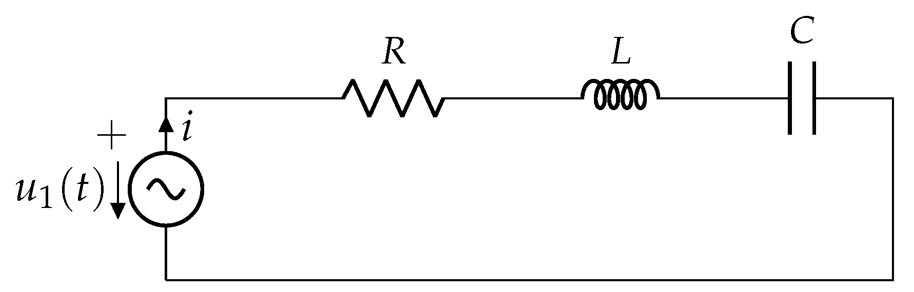
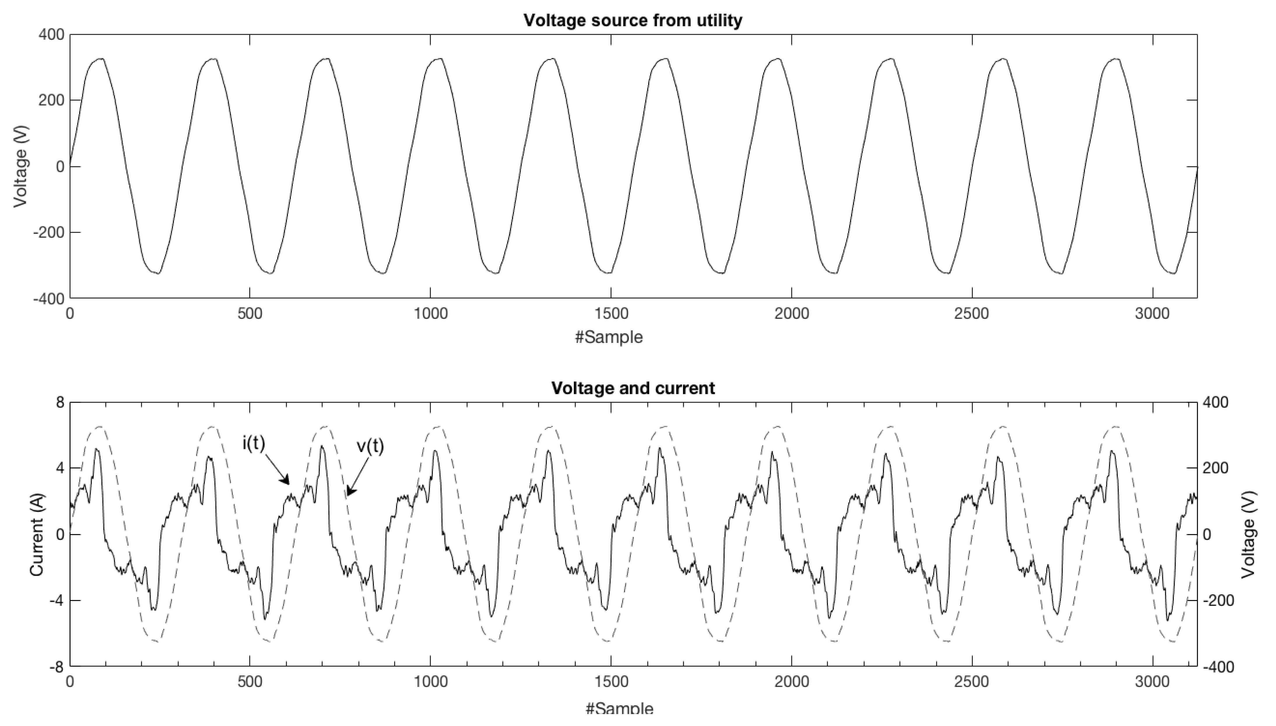
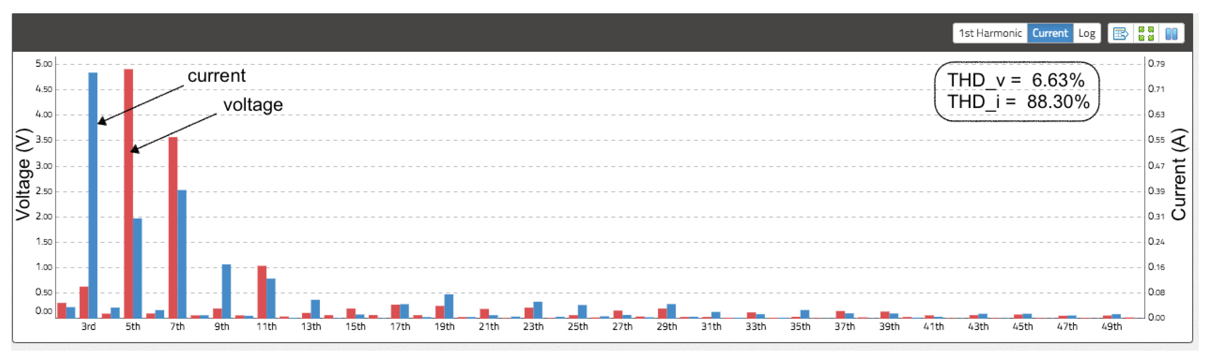
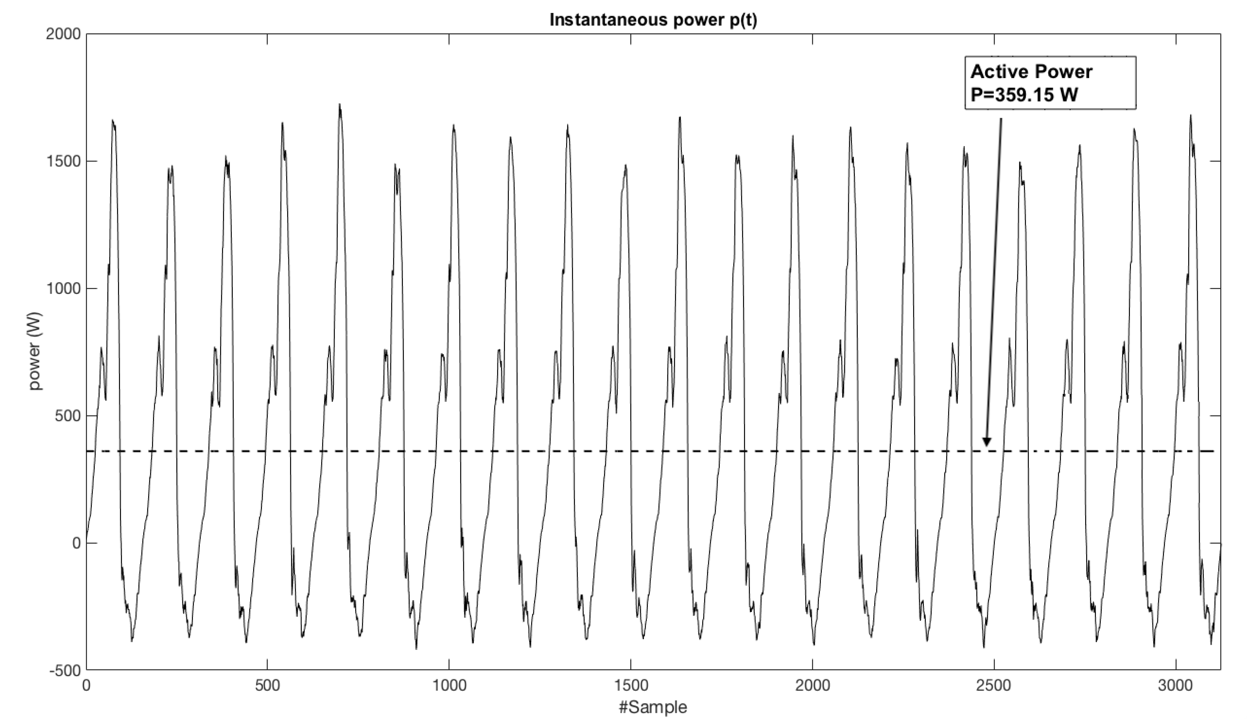
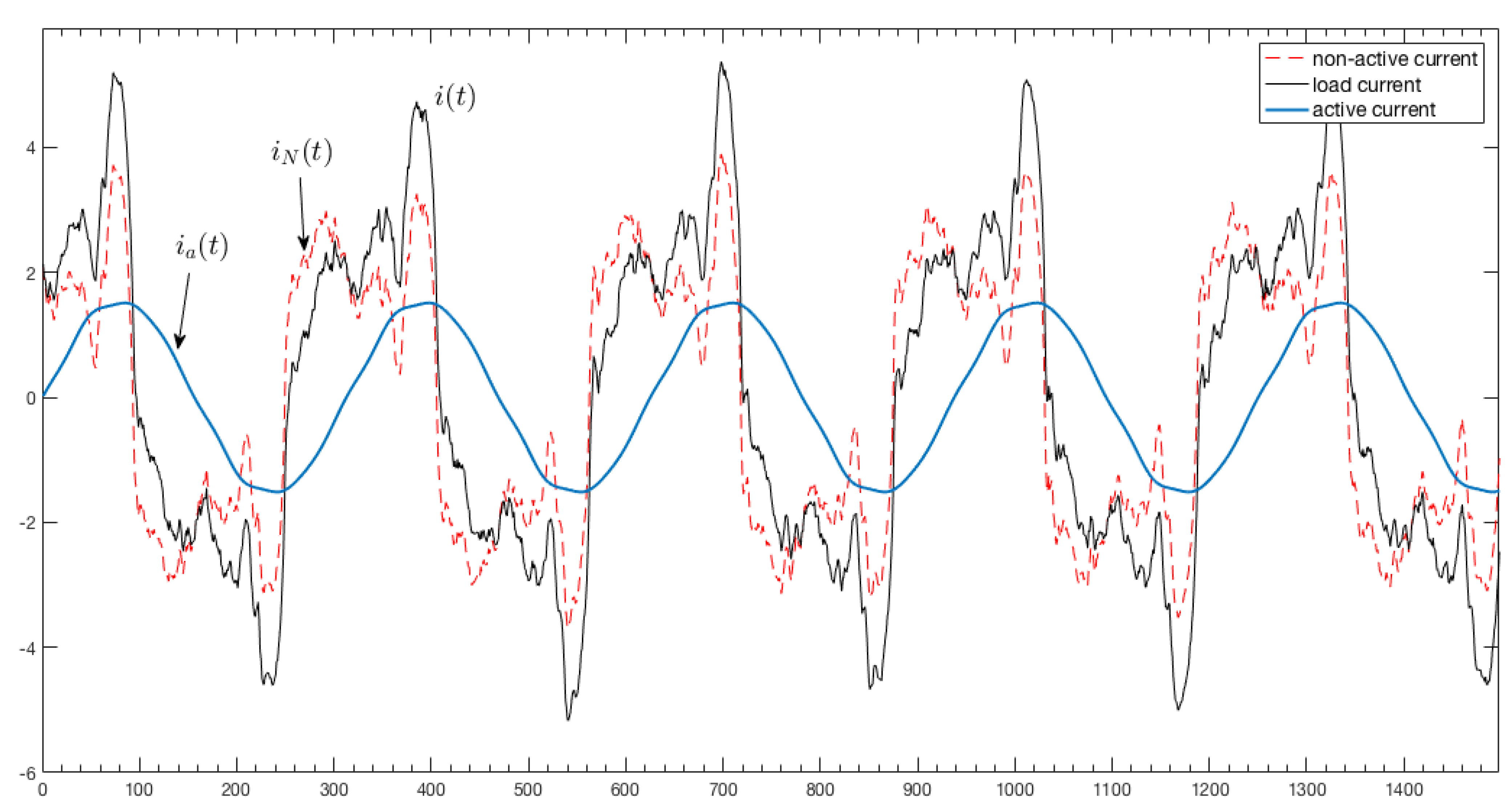
5.2. Example 2: Measurements Analysis

In this example, the voltage and current waveforms of a typical residential building in Almería (Spain) were analysed. The open-platform openZmeter (oZm) was used for the acquisition of the raw values of such waveforms [46]. Figure 3 shows voltage and current measurements in a time window of 200 ms, taken with a sampling frequency of 15.625 kHz (3125 samples). Several home appliances were on, such as a TV and LED lights, or electronic appliances, such as a router, satellite receiver and other devices in stand-by mode. The current waveform was highly distorted since the THDi was 88.3%, while the THDv was 6.63%.

Figure 4 shows the voltage and current spectrum for the first fifty harmonics (for the sake of clarity, the fundamental component is not shown). The fifth and seventh harmonic voltage components were prominent, while even harmonics were insignificant due to the half-wave symmetry of the waveform. From

Table 3. Odd harmonics present in the waveforms of Example 2.

Order	Voltage		Current
	$\parallel \mathit{V}\parallel$ (V)	${\mathit{\phi }}_{\mathit{v}}$ (rad)	$\parallel \mathit{I}\parallel$ (A)	${\mathit{\phi }}_{\mathit{i}}$ (rad)
fund	233.92	−1.57	2.33	−0.72
3rd	0.46	−2.61	0.93	1.85
5th	4.74	1.28	0.45	−1.69
7th	4.02	−0.07	0.49	1.70
9th	0.42	−2.60	0.16	−1.44

, it can be concluded that most of the energy was concentrated in the first five odd harmonics. The RMS value of the voltage was 234.011 V, while that of the current was 2.618A. Figure 5 shows the power waveform, as well as the value of P (359.15 W).

A geometric vector of dimension 100 can be derived, but due to its length, only the five most energetic odd harmonics were selected (the fundamental component plus four odd harmonics), as shown in Table 3. It is worth pointing out that in the proposed theory, the dimension of the geometric space can be chosen according to specific requirements (e.g., the number of harmonics of interest). This is an advantage compared to other theories. In this case, the basis was $\mathit{\sigma }=\{{\mathit{\sigma }}_1,\dots ,{\mathit{\sigma }}_{10}\}$. The voltage and current expressions in polar form are:

$$\begin{array}{cc}\hfill \mathit{u}& =233.92e^{-1.57{\mathit{\sigma }}_{12}}{\mathit{\sigma }}_1+0.46e^{-2.61{\mathit{\sigma }}_{34}}{\mathit{\sigma }}_3+4.74e^{1.28{\mathit{\sigma }}_{56}}{\mathit{\sigma }}_5+4.02e^{-0.07{\mathit{\sigma }}_{78}}{\mathit{\sigma }}_7+0.42e^{-2.60{\mathit{\sigma }}_{\left(9\right)\left(10\right)}}{\mathit{\sigma }}_9\hfill \\ \hfill \mathit{i}& =2.33e^{-0.72{\mathit{\sigma }}_{12}}{\mathit{\sigma }}_1+0.93e^{1.85{\mathit{\sigma }}_{34}}{\mathit{\sigma }}_3+0.45e^{-1.69{\mathit{\sigma }}_{56}}{\mathit{\sigma }}_5+0.49e^{1.70{\mathit{\sigma }}_{78}}{\mathit{\sigma }}_7+0.16e^{-1.44{\mathit{\sigma }}_{\left(9\right)\left(10\right)}}{\mathit{\sigma }}_9\hfill \end{array}$$

(50)

The most significant terms of the geometric power were those related to active and reactive power:

$$\begin{array}{cc}\hfill \mathit{M}& =359.14-408.56{\mathit{\sigma }}_{12}+0.42{\mathit{\sigma }}_{34}+0.34{\mathit{\sigma }}_{56}-1.95{\mathit{\sigma }}_{78}-0.06{\mathit{\sigma }}_{\left(9\right)\left(10\right)}+\mathit{O}\hfill \end{array}$$

(51)

where $\mathit{O}$ includes the rest of the bivectors that appeared due to the cross-frequency products and is not shown due to the lack of space. The norm was $\parallel \mathit{M}\parallel =612.66$ VA, which was nearly the same as $\parallel \mathit{u}\parallel \parallel \mathit{i}\parallel =234.011\times 2.618=612.64$ VA. The value of $M_a$ was $359.21$ W, which was similar to that obtained by using the digital samples of voltages and currents. Results for the reactive power of each harmonic were also similar. Note that the reactive power of the fundamental frequency was encoded in the bivector term ${\mathit{\sigma }}_{12}$. In this case, it had a negative value, so it represented a capacitive behaviour. These values are also shown in

Table 4. Harmonic active (W) and reactive (VAr) power measurements.

Order	${\mathit{P}}_{\mathit{i}}$	${\mathit{Q}}_{\mathit{i}}$
	oZm	oZm	GA
fund	361.80	−408.56	−408.50
3rd	−0.102	0.426	0.425
5th	−2.134	0.346	0.346
7th	−0.408	−1.955	−1.955
9th	0.028	−0.063	−0.062
Total	359.15

.

Table 5. Current components obtained from current measurements.

	${\mathit{i}}_{\mathit{p}}$	${\mathit{i}}_{\mathit{a}}$	${\mathit{i}}_{\mathit{s}}$	${\mathit{i}}_{\mathit{q}}$	${\mathit{i}}_{\mathit{N}}$	i
${\mathit{\sigma }}_1$	−0.007	−0.007	0.000	1.746	1.746	1.739
${\mathit{\sigma }}_2$	1.547	1.534	0.012	0.008	0.020	1.555
${\mathit{\sigma }}_3$	0.188	−0.003	0.190	−0.454	−0.263	−0.266
${\mathit{\sigma }}_4$	−0.108	0.001	−0.109	−0.789	−0.898	−0.897
${\mathit{\sigma }}_5$	−0.126	0.009	−0.135	0.070	−0.065	−0.056
${\mathit{\sigma }}_6$	0.431	−0.030	0.461	0.020	0.482	0.452
${\mathit{\sigma }}_7$	−0.101	0.026	−0.127	0.036	−0.091	−0.065
${\mathit{\sigma }}_8$	−0.007	0.002	−0.010	−0.484	−0.494	−0.492
${\mathit{\sigma }}_9$	−0.057	−0.002	−0.055	0.077	0.022	0.020
${\mathit{\sigma }}_{10}$	0.034	0.001	0.033	0.129	0.162	0.163
$\parallel ·\parallel$	1.629	1.535	0.548	2.035	2.108	2.607

shows the current components presented in Equation (31) for the five most energetic harmonics. In order to compute ${\mathit{i}}_p$ and ${\mathit{i}}_q$ according to Equation (25), the geometric impedances were calculated for each harmonic. The value of the total current was $\parallel \mathit{i}\parallel =2.607$ A, while $\parallel {\mathit{i}}_a\parallel =1.535$ A. Note that the norm of the total current differed slightly from the real one (2.618 A) because not all harmonics were included. It can be observed that $\parallel {\mathit{i}}_a\parallel$ was the minimum current that would produce the same active power. Figure 6 shows the waveforms of $i\left(t\right)$, $i_a\left(t\right)$ and $i_N\left(t\right)$.

6. Conclusions

In this paper, an improved formulation of the power theory based on GA was presented. First, the main shortcomings of existing power theories based on GA were identified. It was shown that the use of k-blades as a basis for the geometric space led to an unclear definition of the geometric apparent power. Moreover, the energy conservation principle cannot be easily fulfilled without extra correction factors. Thus, Menti’s proposal was recovered and favoured for power computations. A new comprehensive isomorphic transformation that accounted for harmonic, sub- and inter-harmonic and DC components’ representation was presented. It simplified the power definitions in the frequency domain and provided a clear meaning to harmonic power. Furthermore, the norm of the geometric power was in good agreement with the traditional definition of apparent power based on the product of RMS voltage and current. Circuit theory analysis can also be performed in the steady state for AC circuits using geometric vectors. The concept of geometric impedance was also introduced with a similar meaning as the well-known complex algebra. It made it possible to analyse electrical circuits by using conventional techniques. Current decomposition for load compensation purposes can be easily carried out by means of the use of the inverse of the current vector. Through different examples, it was shown that the proposed framework overcame some limitations of existing GA-based power theories and provided a comprehensive tool for analysing and solving single-phase electrical circuits under distorted conditions. Moreover, new indices for power quality can be defined based on the suggested non-active power as a result of the cross-frequency products of the voltage and current. Harmonic and power factor correction can also benefit from the proposed approach. Future research is under way to extend this methodology to polyphase systems. This requires the use of orthogonal transformations such as the one derived from the application of the symmetric components. This fact can be addressed through a higher number of dimensions.

References

1. Lee, R.P.; Lai, L.L.; Lai, C.S. Design and Application of Smart Metering System for Micro Grid. In Proceedings of the 2013 IEEE International Conference on Systems, Man, and Cybernetics, Manchester, UK, 13–16 October 2013; pp. 3203–3207. [Google Scholar]
2. Czarnecki, L.S. Currents’ physical components (CPC) in circuits with nonsinusoidal voltages and currents. Part 1, Single-phase linear circuits. Electr. Power Qual. Util. 2005, 11, 3–14. [Google Scholar]
3. Akagi, H.; Watanabe, E.H.; Aredes, M. Instantaneous Power Theory and Applications to Power Conditioning; John Wiley & Sons: Hoboken, NJ, USA, 2017. [Google Scholar]
4. Staudt, V. Fryze-Buchholz-Depenbrock: A time-domain power theory. In Proceedings of the Nonsinusoidal Currents and Compensation, Lagow, Poland, 10–13 June 2008; pp. 1–12. [Google Scholar]
5. Salmerón, P.; Herrera, R.; Vazquez, J. Mapping matrices against vectorial frame in the instantaneous reactive power compensation. IET Electr. Power Appl. 2007, 1, 727–736. [Google Scholar] [CrossRef]
6. Czarnecki, L.S. On some misinterpretations of the instantaneous reactive power pq theory. IEEE Trans. Power Electron. 2004, 19, 828–836. [Google Scholar] [CrossRef]
7. Castro-Nuñez, M.; Castro-Puche, R. The IEEE Standard 1459, the CPC power theory, and geometric algebra in circuits with nonsinusoidal sources and linear loads. IEEE Trans. Circuits Syst. Regul. Pap. 2012, 59, 2980–2990. [Google Scholar] [CrossRef]
8. Chakraborty, S.; Simoes, M.G. Experimental evaluation of active filtering in a single-phase high-frequency AC microgrid. IEEE Trans. Energy Convers. 2009, 24, 673–682. [Google Scholar] [CrossRef]
9. Petroianu, A.I. A geometric algebra reformulation and interpretation of Steinmetz’s symbolic method and his power expression in alternating current electrical circuits. Elec. Eng. 2015, 97, 175–180. [Google Scholar] [CrossRef]
10. Hestenes, D.; Sobczyk, G. Clifford Algebra to Geometric Calculus: A Unified Language for Mathematics and Physics; Springer Science & Business Media: Berlin/Heidelberg, Germany, 2012; Volume 5. [Google Scholar]
11. Ablamowicz, R. Clifford Algebras: Applications to Mathematics, Physics, and Engineering; Springer Science & Business Media: Berlin/Heidelberg, Germany, 2012; Volume 34. [Google Scholar]
12. Easter, R.B.; Hitzer, E. Conic and cyclidic sections in double conformal geometric algebra G 8, 2 with computing and visualization using Gaalop. Math. Methods Appl. Sci. 2020, 43, 334–357. [Google Scholar] [CrossRef]
13. Papaefthymiou, M.; Papagiannakis, G. Real-time rendering under distant illumination with conformal geometric algebra. Math. Methods Appl. Sci. 2018, 41, 4131–4147. [Google Scholar] [CrossRef]
14. Hestenes, D. New Foundations for Classical Mechanics; Springer Science & Business Media: Berlin/Heidelberg, Germany, 2012; Volume 15. [Google Scholar]
15. Dorst, L.; Fontijne, D.; Mann, S. Geometric Algebra for Computer Science: An Object-Oriented Approach to Geometry; Elsevier: Amsterdam, The Netherlands, 2010. [Google Scholar]
16. Chappell, J.M.; Drake, S.P.; Seidel, C.L.; Gunn, L.J.; Iqbal, A.; Allison, A.; Abbott, D. Geometric algebra for electrical and electronic engineers. Proc. IEEE 2014, 102, 1340–1363. [Google Scholar] [CrossRef]
17. Yao, H.; Li, Q.; Chen, Q.; Chai, X. Measuring the closeness to singularities of a planar parallel manipulator using geometric algebra. Appl. Math. Model. 2018, 57, 192–205. [Google Scholar] [CrossRef]
18. Menti, A.; Zacharias, T.; Milias-Argitis, J. Geometric algebra: A powerful tool for representing power under nonsinusoidal conditions. IEEE Trans. Circuits Syst. Regul. Pap. 2007, 54, 601–609. [Google Scholar] [CrossRef]
19. Castilla, M.; Bravo, J.C.; Ordonez, M.; Montaño, J.C. Clifford theory: A geometrical interpretation of multivectorial apparent power. IEEE Trans. Circuits Syst. Regul. Pap. 2008, 55, 3358–3367. [Google Scholar] [CrossRef]
20. Lev-Ari, H.; Stanković, A.M. A geometric algebra approach to decomposition of apparent power in general polyphase networks. In Proceedings of the 41st North American Power Symposium, Starkville, MS, USA, 4–6 October 2009; pp. 1–6. [Google Scholar]
21. Montoya, F.; Baños, R.; Alcayde, A.; Montoya, M.; Manzano-Agugliaro, F. Power Quality: Scientific Collaboration Networks and Research Trends. Energies 2018, 11, 2067. [Google Scholar] [CrossRef] [Green Version]
22. Castro-Núñez, M.; Londoño-Monsalve, D.; Castro-Puche, R. M, the conservative power quantity based on the flow of energy. J. Eng. 2016, 2016, 269–276. [Google Scholar] [CrossRef]
23. Wu, J.C. Novel circuit configuration for compensating for the reactive power of induction generator. IEEE Trans. Energy Convers. 2008, 23, 156–162. [Google Scholar]
24. Castilla, M.; Bravo, J.C.; Ordoñez, M. Geometric algebra: A multivectorial proof of Tellegen’s theorem in multiterminal networks. IET Circuits Devices Syst. 2008, 2, 383–390. [Google Scholar] [CrossRef]
25. Weidmann, J. Linear Operators in Hilbert Spaces; Springer Science & Business Media: Berlin/Heidelberg, Germany, 2012; Volume 68. [Google Scholar]
26. Lev-Ari, H.; Stankovic, A.M. Instantaneous power quantities in polyphase systems—A geometric algebra approach. In Proceedings of the IEEE Energy Conversion Congress and Exposition, San Jose, CA, USA, 20–24 September 2009; pp. 592–596. [Google Scholar]
27. Castro-Núñez, M.; Castro-Puche, R.; Nowicki, E. The use of geometric algebra in circuit analysis and its impact on the definition of power. In Proceedings of the Nonsinusoidal Currents and Compensation (ISNCC), Lagow, Poland, 15–18 June 2010; pp. 89–95. [Google Scholar]
28. Castro-Nuñez, M.; Castro-Puche, R. Advantages of geometric algebra over complex numbers in the analysis of networks with nonsinusoidal sources and linear loads. IEEE Trans. Circuits Syst. Regul. Pap. 2012, 59, 2056–2064. [Google Scholar] [CrossRef]
29. Castro-Núñez, M.; Londoño-Monsalve, D.; Castro-Puche, R. Theorems of compensation and Tellegen in non-sinusoidal circuits via geometric algebra. J. Eng. 2019, 2019, 3409–3417. [Google Scholar] [CrossRef]
30. Montoya, F.G.; Baños, R.; Alcayde, A.; Arrabal-Campos, F.M. A new approach to single-phase systems under sinusoidal and non-sinusoidal supply using geometric algebra. Electr. Power Syst. Res. 2020, 189, 106605. [Google Scholar] [CrossRef]
31. Montoya, F.G.; Baños, R.; Alcayde, A.; Arrabal-Campos, F.M. Analysis of power flow under non-sinusoidal conditions in the presence of harmonics and interharmonics using geometric algebra. Int. J. Elec. Power Energy Sys. 2019, 111, 486–492. [Google Scholar] [CrossRef]
32. Jancewicz, B. Multivectors and Clifford Algebra in Electrodynamics; World Scientific: Singapore, 1989. [Google Scholar]
33. Hitzer, E. Introduction to Clifford’s geometric algebra. arXiv 2013, arXiv:1306.1660. [Google Scholar]
34. Lev-Ari, H.; Stankovic, A.M. A decomposition of apparent power in polyphase unbalanced networks in nonsinusoidal operation. IEEE Trans. Power Sys. 2006, 21, 438–440. [Google Scholar] [CrossRef]
35. Frize, S. Active reactive and apparent power in circuits with nonsinusoidal voltage and current. Elektrotechnische Z. 1932, 53, 596–599. [Google Scholar]
36. Hitzer, E.; Sangwine, S.J. Construction of Multivector Inverse for Clifford Algebras Over 2 m+ 12 m+ 1-Di mensional Vector Spaces fro m Multivector Inverse for Clifford Algebras Over 2 m-Di mensional Vector Spaces. Adv. Appl. Clifford Algebr. 2019, 29, 29. [Google Scholar] [CrossRef] [Green Version]
37. Czarnecki, L.S.; Pearce, S.E. Compensation objectives and Currents’ Physical Components–based generation of reference signals for shunt switching compensator control. IET Power Electron. 2009, 2, 33–41. [Google Scholar] [CrossRef]
38. Shepherd, W.; Zakikhani, P. Suggested definition of reactive power for nonsinusoidal systems. Proc. Inst. Electr. Eng. IET 1972, 119, 1361–1362. [Google Scholar] [CrossRef]
39. Czarnecki, L.S. Considerations on the Reactive Power in Nonsinusoidal Situations. IEEE Tran. Inst. Meas. 1985, IM-34, 399–404. [Google Scholar] [CrossRef]
40. Cohen, J.; De Leon, F.; Hernández, L.M. Physical time domain representation of powers in linear and nonlinear electrical circuits. IEEE Trans. Power Deliv. 1999, 14, 1240–1249. [Google Scholar] [CrossRef]
41. De Léon, F.; Cohen, J. AC power theory from Poynting theorem: Accurate identification of instantaneous power components in nonlinear-switched circuits. IEEE Trans. Power Del. 2010, 25, 2104–2112. [Google Scholar] [CrossRef]
42. Eid, A.H. An extended implementation framework for geometric algebra operations on systems of coordinate frames of arbitrary signature. Adv. Appl. Clifford Algebr. 2018, 28, 16. [Google Scholar] [CrossRef]
43. Sangwine, S.J.; Hitzer, E. Clifford multivector toolbox (for MATLAB). Adv. Appl. Clifford Algebr. 2017, 27, 539–558. [Google Scholar] [CrossRef] [Green Version]
44. Montoya, F.; Alcayde, A.; Arrabal-Campos, F.M.; Baños, R. Quadrature Current Compensation in Non-Sinusoidal Circuits Using Geometric Algebra and Evolutionary Algorithms. Energies 2019, 12, 692. [Google Scholar] [CrossRef] [Green Version]
45. Czarnecki, L. Budeanu and fryze: Two frameworks for interpreting power properties of circuits with nonsinusoidal voltages and currents. Electr. Eng. 1997, 80, 359–367. [Google Scholar] [CrossRef]
46. Viciana, E.; Alcayde, A.; Montoya, F.G.; Baños, R.; Arrabal-Campos, F.M.; Manzano-Agugliaro, F. An Open Hardware Design for Internet of Things Power Quality and Energy Saving Solutions. Sensors 2019, 19, 627. [Google Scholar] [CrossRef] [PubMed] [Green Version]
Figure 1. A vector multiplied by a rotor e φ σ 12 (with positive angle φ ) rotates in the clockwise or counter-clockwise direction depending whether the multiplication is performed by the left or by the right, respectively.
Mathematics 09 01295 g001
Figure 2. R L C circuit used in Example 1.
Mathematics 09 01295 g002
Figure 3. Voltage and current waveform measurements at a residential installation in Spain.
Mathematics 09 01295 g003
Figure 4. Voltage and current spectrum of the waveforms in Figure 3.
Mathematics 09 01295 g004
Figure 5. Instantaneous power waveform and active power P in Example 2.
Mathematics 09 01295 g005
Figure 6. Total, active and non-active current for the measurements.
Mathematics 09 01295 g006