
Multi-Machine Repairable System with One Unreliable Server and Variable Repair Rate

School of Science, Yanshan University, Qinhuangdao 066004, China
Mathematics 2021, 9(11), 1299; https://0-doi-org.brum.beds.ac.uk/10.3390/math9111299
Submission received: 30 April 2021
/
Revised: 31 May 2021
/
Accepted: 2 June 2021
/
Published: 6 June 2021
Abstract
:This paper analyzed the multi-machine repairable system with one unreliable server and one repairman. The machines may break at any time. One server oversees servicing the machine breakdown. The server may fail at any time with different failure rates in idle time and busy time. One repairman is responsible for repairing the server failure; the repair rate is variable to adapt to whether the machines are all functioning normally or not. All the time distributions are exponential. Using the quasi-birth-death(QBD) process theory, the steady-state availability of the machines, the steady-state availability of the server, and other steady-state indices of the system are given. The transient-state indices of the system, including the reliability of the machines and the reliability of the server, are obtained by solving the transient-state probabilistic differential equations. The Laplace–Stieltjes transform method is used to ascertain the mean time to the first breakdown of the system and the mean time to the first failure of the server. The case analysis and numerical illustration are presented to visualize the effects of the system parameters on various performance indices.
1. Introduction
The machine repairing system can be applied to many real systems, such as computer networks, telecommunications, manufacturing systems, aircraft maintenance, and others [1]. Many researchers have studied the multi-server repairable systems [2,3,4,5,6,7]. Wu et al. [8] investigated a machine repair problem with homogeneous machines and standbys available, in which multiple technicians were responsible for supervising these machines and operated a () synchronous vacation policy, the matrix analytical method was employed to obtain a steady-state probability and the closed-form expression of the system performance measures. Chen et al. [9] analyzed the system reliability of the retrial machine repair system with M operating units, S warm standby units, and a single repair server with N-policy. Reliability function and MTTF were derived from Laplace–Stieltjes transform equations. The other works of the single-server models can be referred to [10,11,12,13,14,15]. For the research targets, most of the researchers deal with steady-state characteristics, and some researchers studied transient-state indices [5,16]. Optimizations as the applications of the study also have been done in some research [9,13,17].
It is a fact that a machine may break down in many real systems, and that a machine breakdown can be serviced by a server and resume work again. Furthermore, a server may also fail. When a server fails, a repairman will repair the server failure. Some researchers have studied models in which the server is unreliable, and assumed that the failure rate of the server was a constant value [2,4]. However, in many cases, the system parameters are not fixed due to many working conditions being unstable [14]. It is more reasonable to suppose that the server failure rate is changeable. Some researchers have studied the systems with variable parameters. Yen et al. [18] studied reliability and sensitivity analysis of a retrial machine repair problem with working breakdowns operating under the F-policy. They assumed that the server was subject to working breakdowns only when there was at least one failed machine in the system. When the server is busy, it works at a fast rate, but when it is subject to working breakdowns, it works at a slow rate. The Laplace–Stieltjes transform technique was utilized to develop two system performance measures such as system reliability and the mean time to system failure (MTTF). Meena et al. [19] studied the model in which the repairman may go for a vacation of random length when there are no failed machines queueing up for a repair job. By taking the remaining repair time as a supplementary variable, the steady-state queue size distribution of the number of failed machines in the system was established. Laplace–Stieltjes transform, recursive, and supplementary variable approaches were used to derive various system indices such as the mean queue length, machine availability, system availability, and operative utilization.
In this paper, we consider the repairable system which has multiple machines, one server and one repairman. The machines may break at any time. When a machine is broken, it will be serviced immediately if the server is available, and the machine will continue its work after the service. Further, the server may fail at any time, and the server has different failure rates in idle time and busy time. A repairman is responsible for repairing the server failure, the repair rate is variable to adapt to whether the machines are all normal or not [15]. The distinctive value and novelty of the model is that it simultaneously has features such as multi-machine and an unreliable server, and the breakdown rate and repair rates of the server are variable, so it is a more general model. The previous works may have one or two features similar to our model, but other conditions are significantly different [14,18].
The above system is common in the real world. As an example, multiple computers, one printer (with copy function), and one repairman will constitute such a system. In an office, file editing is the regular work of the computer, and the editing work may be broken by a printing job. If the printing job is seen as a breakdown of the editing work, the printer as a server will service for the breakdown. When the printer is idle, it may do some copy job which can be seen as a failure state of the printer. Moreover, when the printer is doing print work, it may run out of ink or a paper jam may occur, therefore the printer has different failure rates in idle time and busy time. If the print job has non-preemptive priority to the copy job, the printer will do the coming print work first when there is copy job waiting. This means that the failed server has different repair rates which depend on the states of the machines.
This paper achieves the following goals:
- The transition rate matrix and equilibrium equations are given in general forms.
- The steady-state indices and transient-state indices of the system are analyzed.
- Laplace–Stieltjes transform technique is used to derive the reliability indices of the machines and the server in a case analysis; the numerical results are presented.
The rest of this paper is organized as follows: Section 2 describes the model of this paper. Section 3 presents the steady-state performance indices of the system. Section 4 focuses on the transient-state performance indices of the system. Section 5 analyses the reliability of the machine and the server. Section 6 is a case analysis of one machine system. Section 7 gives numerical results for the case of one machine system to illustrate the performance measures of the model and the effects of the parameters.
2. Model Description
The system is constituted by N machines, one server, and one repairman. The machines are charged with the function of the system; every machine is subject to breakdowns according to an independent Poisson process with a rate of . When a machine breaks down, it is immediately serviced by the server if the server is available. Otherwise, the breakdown machines must wait in a queue for the service of the server. The service time for the breakdown machine is exponential distribution with the parameter . The server may fail at any time, the time to failure is exponential distribution with different failures rates which are in idle time and in busy time. When the server fails, the repairman will repair it immediately; the repair time is exponential distribution which the repair rate is when the machines are all normal, and is when at least one machine breaks down. The broken down machine and failure server will become as good as new after servicing and repairing, respectively. All the time distributions are independent mutually.
The running process of the system is a stochastic process which is denoted by , where is the number of available servers at time , and is the number of breakdown machines at time . This stochastic process is a Markov chain with state space . The system is said to be in the state at time if and .
The transient-state probability denoted by , as the state space is finite and irreducible, the limit of exists [9], and the limit is denoted by which is the steady-state probability of the system in the state of .
Then we have
As all the time distributions are exponential distributions and independent mutually, the transitions of the system states form a Markov process which is called the quasi-birth-death(QBD) process [20,21]. The state space of the two-dimensional Markov process, in lexicographical order, is as follows:
Using the analysis method of the QBD theory [16,17,18], we have
where is the higher order infinitesimal of .
Let , we have
where is the derivative of .
In the same way, we obtain:
The above transient-state probabilistic differential equations can be written in a uniform matrix form. Letting
then, we have
where
In the QBD process theory, is called the transition rate matrix.
3. Steady-State Indices
We derive the steady-state probability of the model first in this section. According to the QBD process theory [20,21], we have
We give the notation of the steady-state probability vector as follows:
From the Equation (1), the steady-state equilibrium equations with the regularity condition are as follows:
Solving Equation (2), we obtain the steady-state probabilities of the system. Then the significant steady-state indices of the system are expressed as follows:
- (1)
- The steady-state availability of the system is (The system is available if there is at least one machine available):
- (2)
- The steady-state availability of the server is:
- (3)
- The steady-state probability of the repairman being busy is:
- (4)
- The steady-state probability of the server being busy is:
- (5)
- The steady-state malfunction rate of the machine is:
- (6)
- The steady-state malfunction rate of the server is:
4. Transient-State Indices
This section gives transient-state indices of the system. We assume that the machines and the server are all normal at the initial time. Then, the initial probability vector is as follows:
adding Equation (1), we have:
Using the solutions of Equation (3), corresponding to steady-state indices, the transient-state indices of the system are as follows:
5. Reliability Analysis
5.1. Machine Reliability
We derive transient-state reliability of the machines in this section. We say that the system is available if at least one machine is normal. As the initial condition is that the machines are all normal, the transient reliability of the system at time t denoted by is the probability of the system is available from the beginning time to time t. Letting the states of all the machines break down be the absorbing states, we obtain a new Markov process in which the transition rate matrix is as follows:
Under the initial distribution:
the machine transient-state reliability function is as follows:
where are the solutions of the following equations:
where
5.2. Server Reliability
In this section, we derive the transient-state reliability of the server. The server is normal at the beginning time; the transient reliability of the server at time t denoted by is the probability of the server being available from the beginning time to time t. Letting the states of the server failure be absorbed states, we obtain a new Markov process in which the transition rate matrix is as follows:
where is the element of row 2th and column 2th of matrix .
Under the initial distribution as follows:
the server transient-state reliability function is as follows:
where are solutions of the equations as follows:
where
The mean time to first failure (MTTFF) [16] of the server is as follows:
6. Case Analysis
In this section, we analyze the basic case of of the model, and give numerical examples to illustrate the effects of the system parameters on the performance indices of the system. For the case of , the state space, in lexicographical order, is , and the transition rate matrix is as follows:
6.1. Steady-State Indices of the Case ({N} = 1)
For the case of , the steady-state equilibrium equations are as follows:
Letting
the solutions of Equation (7) are as follows:
Letting and , or letting , we have the results as follows:
The above results are consistent with the case that the server is reliable.
Using steady-state probabilities, we can obtain significant indices of the case as follows:
The Equation (8) shows that the steady-state malfunction rate of the server is equal to the steady-state repair rate of the server. Further, letting and , or letting , we have [22]:
This result is consistent with the result of the classical machine repairable model in which the server is reliable. We know that and or means that the server is reliable, so the availability of the machine only relates to the machine breakdown rate and service rate under those conditions.
6.2. Transient-State Indices of the Case (N = 1)
We assume that the machine and server are normal at the beginning time, so the initial probability vector is as follows:
Under the initial conditions, the transient-state probability equations of the case are as follows:
The symbol express form of the solutions of Equation (9) are very complex; the numerical form solutions can be obtained by mathematical calculation software.
Although the symbol express form of the solutions of Equation (9) are very complex, we can calculate the Laplace–Stieltjes transform of Equation (9). Letting denote the Laplace–Stieltjes transform of , the Laplace–Stieltjes transform of Equation (9) is as follows:
The solutions of Equation (10) are as follows:
where
6.3. Machine Reliability of the Case (N = 1)
For derive transient-state reliability of the machine, we have
Under the initial distribution of and , the machine transient-state reliability denoted by is as follows:
where and are the solutions of the following equations:
The solutions of Equation (11) are as follows:
Then
It is consistent with the assumption that the time of the machine to be broken down is exponential distribution with parameter .
The Laplace–Stieltjes transform of is as follows:
The mean time to first system breakdown (MTTFB) is as follows [16]:
Equation (13) is consistent with Equation (12).
6.4. Server Reliability of the Case (N = 1)
For derive transient-state reliability of the server, we have
Under the initial distribution of and , the server transient-state reliability function denoted by is as follows:
where and are solutions of the equations as follows:
Letting
the solutions of Equation (14) are as follows:
The transient-state reliability function of the server is as follows:
If , Equation (15) will become as follows:
with the assumption of , the reliability of the server has no relation with the parameters and .
The Laplace–Stieltjes transform of Equation (14) is as follows:
the solutions of Equation (17) are as follows:
Then
If , we have
this result is consistent with Equation (16).
6.5. Numerical Example of the Case (N = 1)
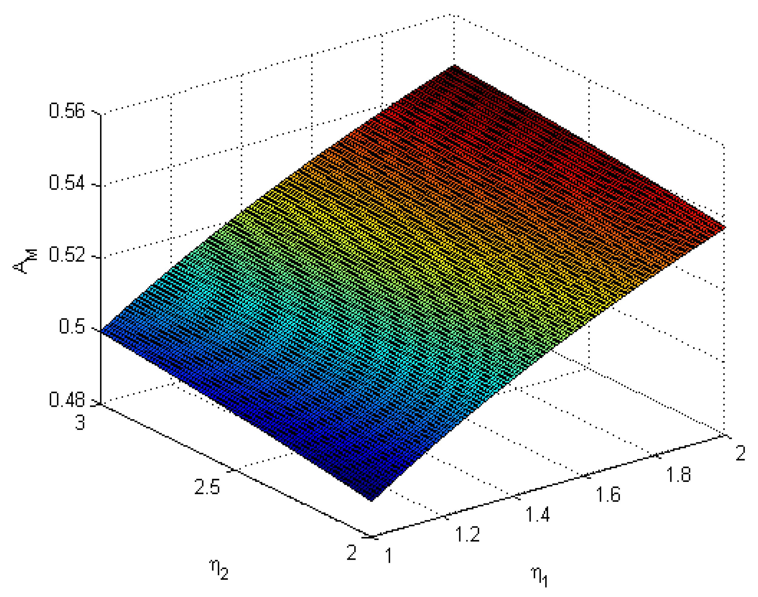
For the case of , letting , , and , Figure 1 shows the numerical results of the steady-state availability of the machine versus and . It is shown that the steady-state availability of the machine increases with the increase of and . Figure 2 shows the numerical results of the steady-state availability of the server versus and . It is shown that the availability of the server increases with the increase in and .
Letting , the initial distribution be , and solving Equation (9), we obtain the transient-state probabilities of the system are as follows:
Using these transient-state probabilities, the transient-state indices of the system are as follows:
As the steady-state probabilities are as follows:
Letting , the steady-state indices of the system are as follows:
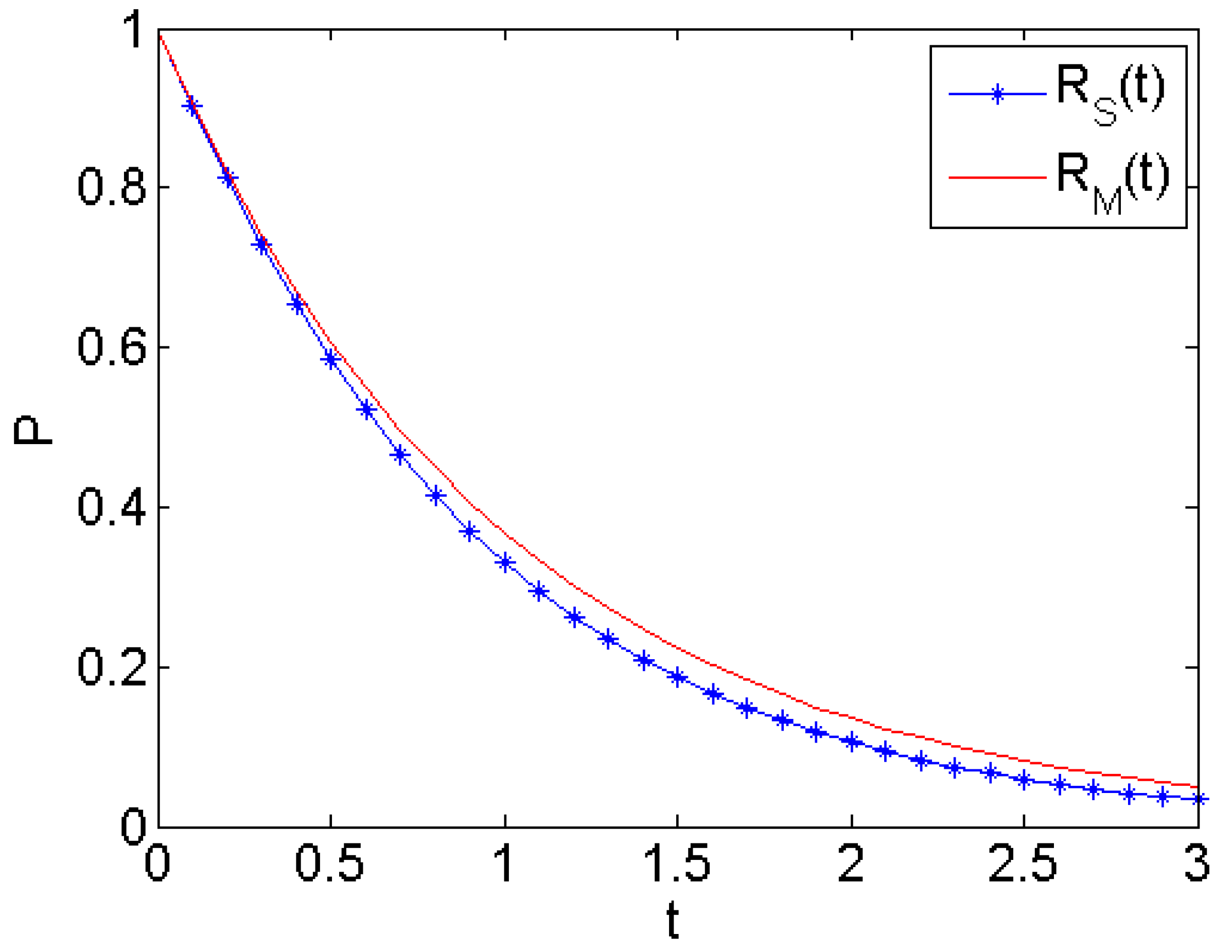
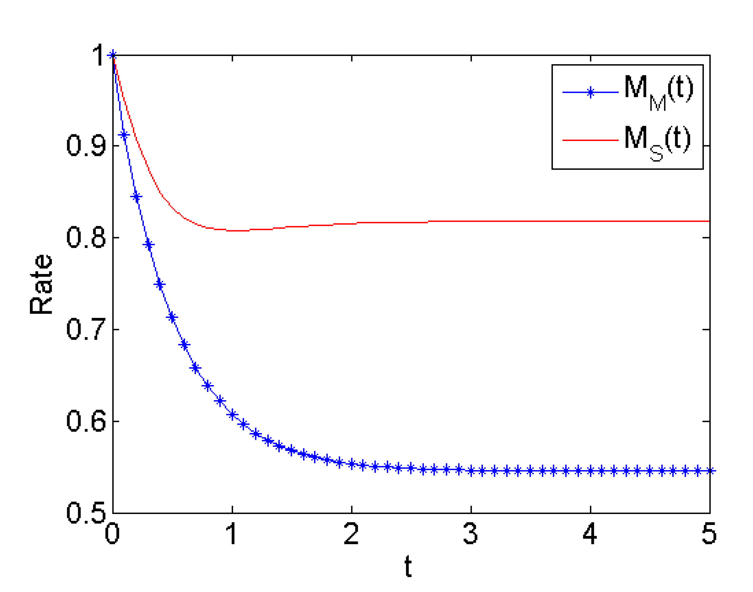
In Figure 3, means that the machine and the server are normal at the beginning time, and means that the repairman is idle at the beginning time. These characters are in accord with the assumption of the initial probabilities. As time goes on, and tend to steady-state values from the initial values. The relation of the repairman being busy is opposite to that of the server being normal due to as shown in Figure 3. Figure 4 shows the reliability of the machine and the reliability of the server versus time t; the reliability of the machine and the reliability of the server all decrease with time t increase. In Figure 5, means that the failure rate of the server is equal to 1 at the beginning time; it is consistent with the assumption of , as the machine is normal and the server is idle at the beginning time; the server malfunction rate of initial time is equal to its idle failure rate . means that the breakdown rate of the machine is equal to 1 at the beginning time; it is consistent with the assumptions of and the machine is normal at the beginning time. and all decrease with time t increase and tend to be steady.
For other numerical results, from Equation (12) we have
this result is consistent with the assumptions of and the machine is normal at the beginning time.
From Equation (15) we have
From Equations (13) and (19) we have
It is shown that the mean time to the first breakdown of the system is equal to 1, and the mean time to first failure of the server is equal to 0.9.
7. Conclusions
The multi-machine repairable system is very common in real practice. The model of this paper with the assumptions that the server is unreliable, and its failure rate and repair rate are variable. These assumptions make the model more general and more suitable for many practical systems. In the case analysis, the explicit expressions of the steady-state and transient-state indices are obtained. Making the different failure rates equal, the results of this model will be reduced to be the results of the model with constant server failure rate. Furthermore, if the repair rates tend to infinity, or the failure rates equate to zero, the results of this model will become the results of a machine repairable model with a reliable server. The numerical examples show that the machine steady-state availability and server steady-state availability all increase with the increases in the two kinds of repair rates. The other steady-state and transient-state indices are also sensitive to the system parameters. These numerical results are instructive to actual production planning and design.
As the server is unreliable, it stands to reason that there are more servers in the system, as well as repairmen. For the future work of this study, one can analyze the model which has many servers and many repairmen. Further, optimization design is an important issue of the model of this paper. The optimal analysis can be a significant direction of the next work of this model.
Funding
This work was supported by the Project of National Natural Science Foundation of China (NO.71971189) and the Project of Natural Science Foundation of Hebei Province (NO. A2020203010).
Institutional Review Board Statement
Not applicable.
Informed Consent Statement
Not applicable.
Data Availability Statement
Not applicable.
Acknowledgments
I am greatly indebted to four anonymous referees for many helpful comments.
Conflicts of Interest
The author declares that he has no conflict of interest.
References
- Haque, L.; Armstrong, M.J. A survey of the machine interference problem. Eur. J. Oper. Res. 2007, 179, 469–482. [Google Scholar] [CrossRef]
- Wang, K. Profit analysis of the M/M/R machine repair problem with spares and server breakdowns. J. Oper. Res. Soc. 1994, 45, 539–548. [Google Scholar] [CrossRef]
- Jain, M.; Maheshwari, S. N-policy for a machine repair systemwith spares and reneging. Appl. Math. Model. 2004, 28, 513–531. [Google Scholar] [CrossRef]
- Jain, M.; Ghimire, R.P. Machine repair queueing system with non-reliable server and heterogeneous services discipline. J. MACT 1997, 30, 105–115. [Google Scholar]
- Jain, M.; Maheshwari, S. Transient analysis of a redundant system with additional repairmen. Amer. J. Math. Manag. Sci. 2003, 23, 347–382. [Google Scholar] [CrossRef]
- Ke, J.C.; Wu, C.H. Multi-server machine repair model with standbys and synchronous multiple vacation. Comput. Ind. Eng. 2012, 62, 296–305. [Google Scholar] [CrossRef]
- Yue, D.Q.; Yue, W.Y.; Qi, H.J. Analysis of a machine repair system with warm spares and N-policy vacations. In Proceedings of the 7th International Symposium on Operations Research and Its Applications (isora’08), Lijiang, China, 31 October–3 November 2008. [Google Scholar]
- Wu, C.H.; Ke, J.C. Multi-server machine repair problems under a (V,R) synchronous single vacation policy. Appl. Math. Model. 2014, 38, 2180–2189. [Google Scholar] [CrossRef]
- Chen, W.L.; Wang, K.H. Reliability analysis of a retrial machine repair problem with warm standbys and a single server with N-policy. Reliab. Eng. Syst. Saf. 2018, 180, 476–486. [Google Scholar] [CrossRef]
- Gupta, U.C.; Srinivasa Rao, T.S.S. On the M/G/1 machine interference model with spares. Eur. J. Oper. Res. 1996, 89, 164–171. [Google Scholar] [CrossRef]
- Lv, S.L.; Xin, X.; Li, J.B.; Hou, Y.M.; Zhao, B. The single machine repairable system with service breakdown. In Chinese Control and Decision Conference; IEEE: New York, NY, USA, 2010; pp. 1480–1483. [Google Scholar]
- Shawky, A.I. The single server machine interference model with balking, reneging and an additional server for longer queues. Microelectron. Reliab. 1997, 37, 355–357. [Google Scholar] [CrossRef]
- Jain, M. Optimal N policy for single server Markovian queue with breakdown, repair and state dependant arrival rate. Int. J. Manag. Syst. 1997, 13, 245–260. [Google Scholar]
- Ouaret, S.; Kenné, J.P.; Gharbi, A. Joint Production and Replacement Planning for an Unreliable Manufacturing System Subject to Random Demand and Quality. IFAC Papers Online 2018, 51, 951–956. [Google Scholar] [CrossRef]
- Van Der Duyn Schouten, F.A.; Wartenhorst, P. A two machine repair model with variable repair rate. Naval Res. Logist. 1993, 40, 495–523. [Google Scholar] [CrossRef] [Green Version]
- Chen, W.L.; Wen, C.H.; Chen, Z.H. System reliability of a machine repair system with a multiple-vacation and unreliable server. J. Test. Eval. 2016, 44, 1745–1755. [Google Scholar] [CrossRef]
- Ke, J.C.; Liu, T.H.; Yang, D.Y. Machine repairing systems with standby switching failure. Comput. Ind. Eng. 2016, 99, 223–228. [Google Scholar] [CrossRef]
- Yen, T.C.; Wang, K.H.; Wu, C.H. Reliability-based measure of a retrial machine repair problem with working breakdowns under the F -policy. Comput. Ind. Eng. 2020, 150, 106885. [Google Scholar] [CrossRef] [PubMed]
- Meena, R.K.; Jain, M.; Sanga, S.S.; Assad, A. Fuzzy modeling and harmony search optimization for machining system with general repair, standby support and vacation. Appl. Math. Comput. 2019, 361, 858–873. [Google Scholar] [CrossRef]
- Ross, S.M. Stochastic Processes; John Wiley and Sons Incorporate: New York, NY, USA, 1983; pp. 162–211. [Google Scholar]
- Neuts, M.F. Matrix-Geometric Solutions in Stochastic Models; The Johns Hopkins University Press Ltd.: London, UK, 1981; pp. 254–300. [Google Scholar]
- Cao, J.H. Introduction to Reliability Mathematics; Science Press: Beijing, China, 2012; pp. 189–220. [Google Scholar]
Figure 1.
The steady-state availability of the machine for and .

Figure 2.
The steady-state availability of the server for and .

Figure 3.
The transient-state indices of the system for and .

Figure 4.
The transient-state reliability functions of the machine and the server for and .

Figure 5.
The transient-state malfunction rate of the machine and the server for and .

Publisher’s Note: MDPI stays neutral with regard to jurisdictional claims in published maps and institutional affiliations. |
© 2021 by the author. Licensee MDPI, Basel, Switzerland. This article is an open access article distributed under the terms and conditions of the Creative Commons Attribution (CC BY) license (https://creativecommons.org/licenses/by/4.0/).
Share and Cite
MDPI and ACS Style
Lv, S. Multi-Machine Repairable System with One Unreliable Server and Variable Repair Rate. Mathematics 2021, 9, 1299. https://0-doi-org.brum.beds.ac.uk/10.3390/math9111299
AMA Style
Lv S. Multi-Machine Repairable System with One Unreliable Server and Variable Repair Rate. Mathematics. 2021; 9(11):1299. https://0-doi-org.brum.beds.ac.uk/10.3390/math9111299
Chicago/Turabian StyleLv, Shengli. 2021. "Multi-Machine Repairable System with One Unreliable Server and Variable Repair Rate" Mathematics 9, no. 11: 1299. https://0-doi-org.brum.beds.ac.uk/10.3390/math9111299
Note that from the first issue of 2016, this journal uses article numbers instead of page numbers. See further details here.